Dynamic Isoline Extraction
for Visualization of Streaming Data
Dina Goldin1
, Huayan Gao University of Connecticut, Storrs, CT USA
{dqg,ghy}@engr.uconn.edu
Abstract. Queries over streaming data offer the potential to provide timely in-formation for modern database applications, such as sensor networks and web services. Isoline-based visualization of streaming data has the potential to be of great use in such applications. Dynamic (real-time) isoline extraction from the streaming data is needed in order to fully harvest that potential, allowing the users to see in real time the patterns and trends – both spatial and temporal – inherent in such data. This is the goal of this paper.
Our approach to isoline extraction is based on data terrains, triangulated irregular networks (TINs) where the coordinates of the vertices corresponds to locations of data sources, and the height corresponds to their readings. We dynamically maintain such a data terrain for the streaming data. Furthermore, we dynamically maintain an isoline (contour) map over this dynamic data network. The user has the option of continuously viewing either the current shaded triangulation of the data terrain, or the current isoline map, or an overlay of both.
For large networks, we assume that complete recomputation of either the data terrain or the isoline map at every epoch is impractical. Ifnis the number of data sources in the network, time complexity per epoch should beO(log n)to achieve real-time performance. To achieve this time complexity, our algorithms are based on efficient dynamic data structures that are continuously updated rather than recomputed. Specifically, we use a doubly-balanced interval tree, a new data structure where both the tree and the edge sets of each node are balanced. As far as we know, no one has applied TINs for data terrain visualization before this work. Our dynamic isoline computation algorithm is also new. Experimental results confirm both the efficiency and the scalability of our approach.
1
Introduction
Queries over streaming data offer the potential to provide timely information for mod-ern database applications, such as sensor networks and web services. Isoline-based vi-sualization of streaming data has the potential to be of great use in such applications. Isoline (contour) maps is particularly informative if the streaming data values are related to phenomena that tend to be continuous for any given location, such as temperature, pressure or rainfall in a sensor network.
Dynamic (real-time) isoline extraction from the streaming data is needed in order to allow the users to see in real time the patterns and trends – both spatial and temporal – inherent in such data. Such isoline extraction is the goal of this paper.
Our approach to isoline extraction is based on data terrains, triangulated irregular networks (TINs) where the(x, y)-coordinates of the vertices corresponds to locations of data sources, and thez-coordinate corresponds to their readings. Efficient algorithms, especially when implemented in hardware, allow for fast shading of TINs, which are three-dimensional. By combining shading with user-driven rotation and zooming, data terrains provide a very user-friendly way to visualize data networks.
While the rendering of static TINs is a well-researched problem, we are concerned with dynamic networks, where data sources may change their readings over time; they may also join the network, or leave the network. We dynamically maintain a data terrain for the streaming data from such a network of data sources.
Furthermore, we dynamically maintain an isoline (contour) map over this dynamic data network. Isolines consist of points of equal value; they are most commonly used to map mountainous geography. The isoline map can be displayed in isolation, or over-layed on the underlying TIN, providing the user with a visualization that is both highly descriptive and very intuitive.
For large networks, we assume that complete recomputation of either the data ter-rain or the isoline map at every epoch is impractical. Ifnis the number of data sources in the network, time complexity per epoch should be O(log n)to achieve real-time performance. To achieve this time complexity, our algorithms are based on efficient dynamic data structures that are continuously updated rather than recomputed. Specifi-cally, we use a doubly-balanced interval tree, a new data structure where both the tree and the edge sets of each node are balanced.
Dynamic isoline maps have been proposed before in the context of sensor net-works [7, 11]. However, as far as we know, no one has applied TINs for this purpose before this work. Our dynamic isoline computation algorithm is also new. As a result, earlier approaches produce isoline maps that are in both more costly and less accurate. We have implemented the data structures and algorithms proposed in the paper. The user has the option of continuously viewing either the current shaded triangulation, or the current isoline map, or an overlay of both. Experimental results, simulating a large network of randomly distributed data sources, confirm both the efficiency and the scalability of our approach.
Overview. We describe data terrains in section 2, and discuss the algorithms for their computation and dynamic maintenance. In section 3, we give an algorithm for comput-ing isoline maps over the data terrain, as well as their dynamic maintenance. In section 4 we present our implementation of isoline-based visualization. Related work is dis-cussed in section 5, and we conclude in section 6.
2
Data Terrains
Our notion of a data terrain is closely related to the notion of a geographic terrain, com-monly used in Geographic Information Systems (GIS). Geographic terrains represent elevations of sites and are static.
There are two main approaches to represent terrains in GIS. One is Digital Elevation
Models (DEM), representing it as gridded data within some predefined intervals, which
the regularity of DEMs, they are not appropriate for networks of streaming data sources, whose locations are not assumed to be regular. The other representation is Triangulated
Irregular Networks (TIN). The vertices of a TIN, sometimes called sites, are distributed
irregularly and stored with their location(x, y)as well as their height valuezas vector
data(x, y, z); TINs are typically used in vector data models. For a detailed survey of
terrain algorithms, including TINs, see [17].
In this paper, we chose to use TINs to represent the state of a data network. TINs are good for visualization, because they can be efficiently shaded to highlight the 3D aspects of the data. The (x, y)coordinates of the TIN’s vertices corresponds to the locations of data sources, and thezcoordinates corresponds to their current value (that is being visualized). We refer to this representation as data terrains.
We initially construct the data terrain with the typical algorithm for TIN construc-tion, as in [8, 9] inO(n log n)time. Since the construction of TIN is only dependent on the location of its sites, the topology of the TIN does not change with the change of the data values. The only possibility for a TIN to change is when a new data source joins the network, or when some data source leaves the network, e.g. due to power loss. In the following, we describe the algorithm for updating the TIN when this happens. Insertion. When a new data source is added to the network, we need to add the cor-responding vertex to the data terrain. It would be the same algorithm as when building a new data terrain, since it is an incremental algorithm. As discussed in [9], the worst case of the time performance for site insertion could beO(n). Note that we assume that data sources are not inserted often, much less frequently than their values are updated, giving us amortized performance ofO(log n)for this operation.
Deletion. When a data source leaves the network, we need a local updating algorithm to maintain our dynamic TIN. Basically, this is the inverse of the incremental insertion algorithm, but in practice there are a variety of specific considerations. [10] first de-scribed a deletion algorithm in detail, but unfortunately, it had mistakes. The algorithm was corrected in [5], and further improved in [14]. The performance for deletion algo-rithm isO(k log k)wherekis the number of neighbors of the polygon incident the vertex to be deleted. Figure 1 illustrates how one site is removed from a TIN.
Efficient algorithms, especially when implemented in hardware, allow for fast shad-ing of data terrains. By combinshad-ing shadshad-ing with user-driven rotation and zoomshad-ing, data terrains provide a very user-friendly way to visualize data networks.
3
Dynamic Isoline Extraction
In this section, we describe how to extract an isoline map from a data terrain for a dynamic data network.
3.1 Interval tree
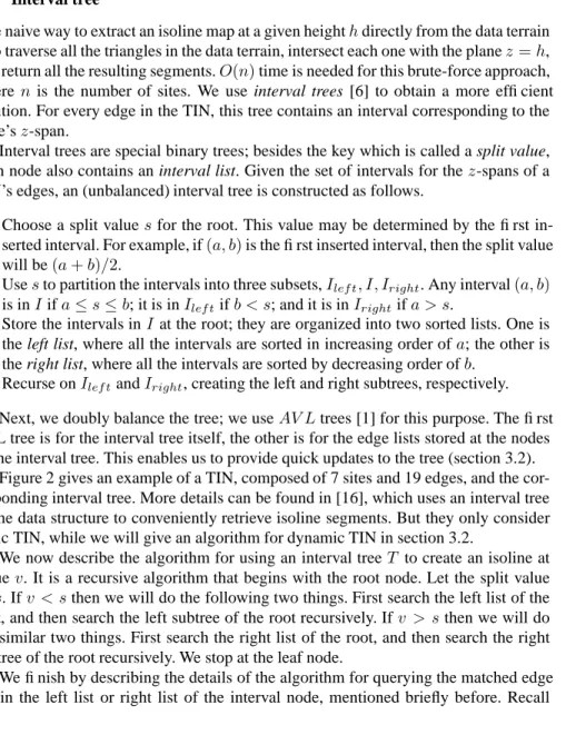
One naive way to extract an isoline map at a given heighthdirectly from the data terrain is to traverse all the triangles in the data terrain, intersect each one with the planez=h, and return all the resulting segments.O(n)time is needed for this brute-force approach, wheren is the number of sites. We use interval trees [6] to obtain a more efficient solution. For every edge in the TIN, this tree contains an interval corresponding to the edge’sz-span.
Interval trees are special binary trees; besides the key which is called a split value, each node also contains an interval list. Given the set of intervals for thez-spans of a TIN’s edges, an (unbalanced) interval tree is constructed as follows.
1. Choose a split valuesfor the root. This value may be determined by the first in-serted interval. For example, if(a, b)is the first inserted interval, then the split value will be(a+b)/2.
2. Usesto partition the intervals into three subsets,Ilef t, I, Iright. Any interval(a, b)
is inIifa≤s≤b; it is inIlef tifb < s; and it is inIrightifa > s.
3. Store the intervals inI at the root; they are organized into two sorted lists. One is the left list, where all the intervals are sorted in increasing order ofa; the other is the right list, where all the intervals are sorted by decreasing order ofb.
4. Recurse onIlef tandIright, creating the left and right subtrees, respectively.
Next, we doubly balance the tree; we useAV Ltrees [1] for this purpose. The first AVL tree is for the interval tree itself, the other is for the edge lists stored at the nodes of the interval tree. This enables us to provide quick updates to the tree (section 3.2).
Figure 2 gives an example of a TIN, composed of 7 sites and 19 edges, and the cor-responding interval tree. More details can be found in [16], which uses an interval tree as the data structure to conveniently retrieve isoline segments. But they only consider static TIN, while we will give an algorithm for dynamic TIN in section 3.2.
We now describe the algorithm for using an interval treeT to create an isoline at valuev. It is a recursive algorithm that begins with the root node. Let the split value
bes. Ifv < sthen we will do the following two things. First search the left list of the
root, and then search the left subtree of the root recursively. Ifv > sthen we will do the similar two things. First search the right list of the root, and then search the right subtree of the root recursively. We stop at the leaf node.
We finish by describing the details of the algorithm for querying the matched edge list in the left list or right list of the interval node, mentioned briefly before. Recall
0 52.9 0.2 12.4 279.5 136.3 27.6 a b c d e f g h i j k l m n d d 0.1 139.85 6.3 74.35 32.65 g, i, m m, g, i 0 30 60 90 120 150 180 210 240 270 300 a b c d e f g h i j n k l m c, e, n c, e, n f, h f, h a, b, j, k, l b, l, j, k, a
Fig. 2. An example of a TIN and the corresponding balanced interval tree.
that we stored the edge list as anAV Ltree. Take the left list as an example, we only consider the left evaluation of the smaller point of the edge. Let it be the keykof the
AV L node. We search the AV Ltree recursively. If v < k, then we search the left subtree recursively. Ifv > k, which means that all the edges in the left subtree are the matched edges, output them and search the right subtree recursively. Querying the right list of the interval node is symmetric.
Note that an interval tree can also be constructed for triangles, rather than edges, of the TIN, since az-span can just as easily be defined for triangles. We can quickly find those triangles that intersect with the planez =h, and avoid considering others. One such algorithm is given in [16].
In our work, we found it more convenient to use edges to compute isolines from the TIN instead of triangles. Note that this kind of substitution does not affect the efficiency, because of the following fact: if there arenvertices in the TIN, the number of edges
and the number of triangles are eachO(n)[13]. Letnbdenote the number of sites on
the boundary of the TIN, andnibe the number of sites in the interior; the total number
of sites isn =nb+ni. The number of edges isne= 2nb+ 3(ni−1)<= 3n. The
number of triangles, let bent, would bent = 2n−6whenn >3. Therefore, both the
edge-based and the triangle-based interval trees allow for a more efficient algorithm to get the isolines from TIN than the naive one described at the beginning of the section.
3.2 Dynamic Interval Tree
In our setting, the data values at the sources change as time passes. Since our interval tree is built up on the edges of the TIN, and thez-span of the edge is dependent on the values at the sites adjacent to the edge, a change in these values will necessitate a change to the interval tree.
We begin with a built TIN and a constructed interval tree, as described above. In the following, we give a detailed description of the algorithm to update the tree after some data sourceschanges its value fromv0tov.
1. We use the TIN to find all edges incident with the data sources. Since the TIN contains an incidence listLfor each vertex, we can find these edges in constant timeO(1).
2. For every edgeein the listL, we need to update its position in the interval tree. Suppose that the originalz-span foreisze, and the new one isze0.
3. Run a binary search from the root to find the nodexwhich contains the intervalze.
This is done inO(log n)time.
4. Deletezefrom both the right and the left lists ofx. Since both of these lists are
implemented as a standard AVL tree, the performance isO(log n). 5. Look for the nodeythat should containz0
e, that is, its split value overlapsze0. First,
check whetherz0
e overlaps with the split value ofx, in which case we need look
no further. Otherwise, begin searching from the root of the tree, comparingz0
ewith
the split value of the node, until we find the node whose split value overlapsz0
eor
reach a leaf. The time for this is inO(log n). 6. If we foundy, then insertz0
e into the right and the left lists ofy. Both lists are
implemented with AVL trees, and the size of each list is at most the total number of the edges in the TIN. So this insert should be inO(log n).
7. If we have reached a leaf without findingy, we insert a new leaf into the interval tree to store the new interval. Its interval lists will contain justz0
e, and its split value
will be the midpoint ofz0
e; this is inO(1).
Recall that we are using balanced (AVL) trees both for the interval tree, and for the interval lists within each node of the interval tree. To keep the trees balanced, all insertions and deletions are followed by a rebalance operation. There exists the rebal-ance algorithm for AVL trees inO(log n)time [19], and it is easy to see that double balancing does not increase the time complexity. An alternative method is relaxed AVL
tree [12]. Instead of rebalancing the tree at every update, we relax the restriction and
accumulate a greater difference is heights before we need to adjust the height of the AVL tree.
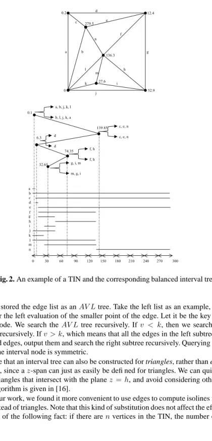
Figure 3illustrates an update to the interval tree of Figure 2 when the reading of data sourceschanges from136.3to170.4. Note that all edges incident onsneed to be checked. In this figure, we need to update the position of intervalsf, h, l, m, nin the interval tree. d d 0.1 139.85 6.3 224.95 74.35 32.65 g, i g, i 0 30 60 90 120 150 180 210 240 270 300 a b c d e f g h i j n k l m c, e, f, m, h c, e, f, h, m n n a, b, j, k, l b, l, j, k, a
Fig. 3. An update to the interval tree.
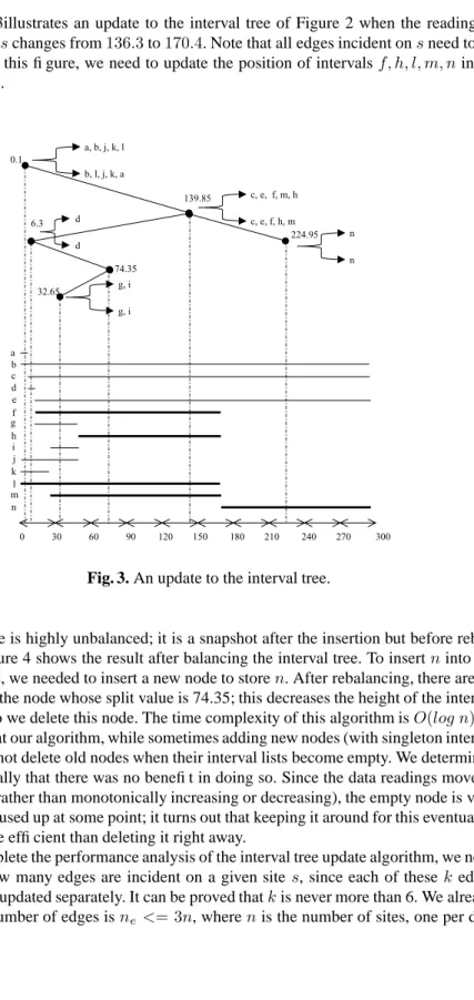
This tree is highly unbalanced; it is a snapshot after the insertion but before rebal-ancing. Figure 4 shows the result after balancing the interval tree. To insertninto the interval tree, we needed to insert a new node to storen. After rebalancing, there are no intervals in the node whose split value is 74.35; this decreases the height of the interval tree by 1, so we delete this node. The time complexity of this algorithm isO(log n).
Note that our algorithm, while sometimes adding new nodes (with singleton interval lists), does not delete old nodes when their interval lists become empty. We determined experimentally that there was no benefit in doing so. Since the data readings move up and down (rather than monotonically increasing or decreasing), the empty node is very likely to be used up at some point; it turns out that keeping it around for this eventuality is more time efficient than deleting it right away.
To complete the performance analysis of the interval tree update algorithm, we need to know how many edges are incident on a given site s, since each of thesekedges needs to be updated separately. It can be proved thatkis never more than 6. We already know the number of edges isne <= 3n, wherenis the number of sites, one per data
k, d k, d 32.65 6.3 139.85 0.1 224.95 b, j, l, c, e, f, g, i, m b, c, e, f, l, m, g, i, j 0 30 60 90 120 150 180 210 240 270 300 a b c d e f g h i j n k l m h h n n a a
Fig. 4. The updated interval tree after rebalancing.
source. Since each edge is incident on two sites, clearly we have:k= 2∗ne
n <= 6. We
confirmed this experimentally, measuring the average ofk; we found that it was never more than6, not growing as the number of sites increased. Therefore, we assume thatk
isO(1).
For each edge, we took itsz-span interval from its old position and found an ap-propriate new position to insert the interval, rebalancing when needed. Each of these operations is inO(log n)time. Therefore, the overall algorithm isO(log n).
4
Performance
4.1 Assumptions
Our visualization algorithm relies on continuously updating the TIN and the corre-sponding interval tree. The updates are triggered by changes to data values, insertions (new data sources), or deletions (loss of a data source). We use the amortized approach to complexity analysis, assuming that changes to data values happen much more often than either insertions or deletions.
4.2 Experiments
Our implementation of the visualization of data terrain uses OpenGL [15], a software interface to graphics hardware. In our simulation, we used GNU C++ with OpenGL
library under Linux platform to render the data terrain and isoline maps. We imple-mented isoline extraction from data terrains using the algorithm described above. In our experiment, we started by generating the initial data terrain from the initial values at data sources, using the algorithm in section 2. Then we constructed our interval tree using the algorithm in section 3.
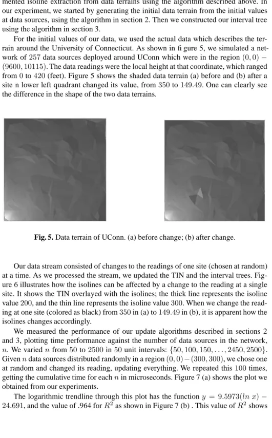
For the initial values of our data, we used the actual data which describes the ter-rain around the University of Connecticut. As shown in figure 5, we simulated a net-work of257data sources deployed around UConn which were in the region(0,0)−
(9600,10115). The data readings were the local height at that coordinate, which ranged from0to420(feet). Figure 5 shows the shaded data terrain (a) before and (b) after a site n lower left quadrant changed its value, from350to149.49. One can clearly see the difference in the shape of the two data terrains.
Fig. 5. Data terrain of UConn. (a) before change; (b) after change.
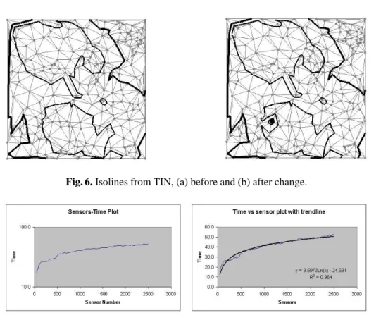
Our data stream consisted of changes to the readings of one site (chosen at random) at a time. As we processed the stream, we updated the TIN and the interval trees. Fig-ure 6 illustrates how the isolines can be affected by a change to the reading at a single site. It shows the TIN overlayed with the isolines; the thick line represents the isoline value200, and the thin line represents the isoline value300. When we change the read-ing at one site (colored as black) from350in (a) to149.49in (b), it is apparent how the isolines changes accordingly.
We measured the performance of our update algorithms described in sections 2 and 3, plotting time performance against the number of data sources in the network,
n. We variednfrom50to2500in50unit intervals:{50,100,150, . . . ,2450,2500}. Givenndata sources distributed randomly in a region(0,0)−(300,300), we chose one at random and changed its reading, updating everything. We repeated this100times, getting the cumulative time for eachnin microseconds. Figure 7 (a) shows the plot we obtained from our experiments.
The logarithmic trendline through this plot has the functiony = 9.5973(ln x)−
24.691, and the value of .964 forR2
as shown in Figure 7 (b) . This value ofR2 shows
Fig. 6. Isolines from TIN, (a) before and (b) after change.
Fig. 7. Time performance vs. number of sites, (a) without and (b) with the logarithmic trendline.
that there is a96.4%reliability of the relationship between the plot and the trendline. From this picture, we can see that our algorithm is logarithmic and scalable. This con-firms our analysis in section 3.
5
Related work
The visualization of data terrains involves much knowledge in computer graphics. A good review of rendering techniques such as transformations, shading, interpolation, texture mapping, ray tracing, etc., as well as the mathematics theory behind it, can be found in [18, 2]. One of the popular rendering libraries is OpenGL. It is said to be industry standard; it is stable, reliable, portable, extensible, scalable and easy to use. Documents are available from http://www.opengl.org. [15], written by the OpenGL Architecture Review Board, is the most authoritative one. In our simulation, we used GNU C++ with OpenGL under Linux to render our data terrain and our isoline map.
Interval tree first was propose by Edelsbrunner [6] to efficiently retrieve intervals of real lines that contain a given query value. Cignoni et. al. [4] uses interval tree as
the data structure to extract isosurfaces. Chiang [3] describes how to extract isosurface from volumetric data using interval tree.
Van Kreveld [16] uses the interval tree as the data structure to extract isolines from TINs by associating each triangle with the intervals of the elevation it spans. There are several differences between that algorithm and ours. Their intervals are based on
z-spans of triangles rather than edges. They do not use balanced trees as we do. Their algorithm is not dynamic (the update operations are not defined). Finally, as far as we know, their algorithm was never implemented.
To our knowledge, no one has described an algorithm to extract isolines efficiently and dynamically from data terrains as we have done. Related work in the sensor net-work community has tried to extract isolines directly from sensor readings, using in-network protocols. For example, in [11], an isobar computation from sensor in-networks is performed as a form of aggregation. This work assumes that every sensor is in a rectangular grid and merge these grids in-network. The communication between the sensors is based on a tree. The general process is that each sensor gets the isobar map from its children, combines its own information, and sends the isobar map up to its par-ent. Finally, the root aggregates the isobar maps. So they need some polygon operations such as intersect and union; the time complexity isO(n log n), wherenis the number of edges in the polygon. Whenever there are some sensors changing their reading, we need to compute the isobar again, so this approach is not efficient in a dynamic real-time setting.
6
Conclusions
Isoline-based visualization of streaming data has the potential to be of great use in modern database applications, such as sensor networks and web services. This paper was concerned with dynamic (real-time) isoline extraction from the streaming data, so as to allowing the users to see in real time the patterns and trends – both spatial and temporal – inherent in such data.
Our approach to isoline extraction was based on data terrains, triangulated irregular networks (TINs) where the coordinates of the vertices corresponds to locations of data sources, and the height corresponds to their readings. We dynamically maintained such a data terrain for the streaming data. Furthermore, we dynamically maintained an isoline (contour) map over this dynamic data network.
For large networks, we assumed that complete recomputation of either the data ter-rain or the isoline map at every epoch is impractical. Ifnis the number of data sources in the network, time complexity per epoch should be O(log n)to achieve real-time performance. To achieve this time complexity, our algorithms are based on efficient dynamic data structures that are continuously updated rather than recomputed. Specifi-cally, we used a doubly-balanced interval tree, a new data structure where both the tree and the edge sets of each node are balanced.
As far as we know, no one has applied TINs for data terrain visualization before this work. Our dynamic isoline computation algorithm is also new. Experimental results confirm both the efficiency and the scalability of our approach. All our implementation was in GNU C++ with OpenGL library under Linux.
References
1. G.M. Adelson-Velskii and E.M. Landis. An algorithm for the organization of information.
In Soviet Math. Doclady 3, pages 1259–1263, 1962.
2. Edward Angel. Interactive Computer Graphics: A Top-Down Approach with OpenGL. Pear-son AddiPear-son-Wesley, Jul. 2002.
3. Yi-Jen Chiang and Claudio T. Silva. I/O Optimal Isosurface Extraction. IEEE Visualization
’97, pages 293–250, 1997.
4. Paolo Cignoni, Paola Marino, Claudio Montani, Enrico Puppo, and Roberto Scopigno. Speeding up Isosurface Extraction Using Interval Tree. IEEE Trans. on Visualization and
Computer Graphics, 3, Apr.-Jun. 1997.
5. Olivier Devillers. On Deletion in Delaunay Triangulations. Proc. 15th Annual Symp. on
Computational Geometry, pages 181–188, Jun. 1999.
6. Edelsbrunner. Dynamic Data Structure for Orthogonal Intersection Queries. Tech. Rep. F59,
Inst. Informationsverarb. Tech. Univ. Graz, Graz, Austria, 1980.
7. Deborah Estrin. Embedded Networked Sensing for Environmental Monitoring: Applications and Challenges. DIALM-POMC Joint Workshop on Found. of Mobile Computing, San Diego,
CA, Sep. 2003.
8. Michael Garland and Paul S. Heckbert. Fast Polygonal Approximations of Terrains and Height Fields. Tech. Rep. CMU-CS-95-181, Carnegie Mellon Univ., Sep. 1995.
9. Leonidas Guibas and Jorge Stolfi. Primitives for the Manipulation of General Subdivisions and the Computation of Vorono Diagrams. ACM Trans. on Graphics, 4(2):74–123, 1985. 10. Martin Heller. Triangulation Algorithms for Adaptive Terrain Modeling. Proc. 4th Int’l
Symp. of Spatial Data Handling, pages 163–174, 1990.
11. Joseph M. Hellerstein, Wei Hong, Samuel Madden, and Kyle Stanek. Beyond Average: Towards Sophisticated Sensing with Queries. 2nd Int’l Workshop on Information Proc. in
Sensor Networks (IPSN ’03), Mar. 2003.
12. Kim S. Larsen, Eljas Soisalon-Soininen, and Peter Widmayer. Relaxed Balance through Standard Rotations. Workshop on Alg. and Data Structures, 1997.
13. Charles L. Lawson. Software forC1Surface Interpolation. In John R. Rice, ed.,
Mathemat-ical Software III, Academic Press, NY, pages 161–194, 1977.
14. Mir Abolfazl Mostafavi, Christopher Gold, and Maciej Dakowicz. Delete and Insert Op-erations in Voronoi / Delaunay Methods and Applications. Computers & Geosciences,
29(4):523–530, May 2003.
15. Dave Shreiner, Mason Woo, Jackie Neider, and Tom Davis. OpenGL Programming Guide:
The Official Guide to Learning OpenGL, Version 1.4, 4th edition. Addison-Wesley, Nov.
2003.
16. Marc van Kreveld. Efficient Methods for Isoline Extraction from a Digital Elevation Model Based on Triangulated Irregular Networks. In 6th Int’l Symp. on Spatial Data Handling
Proc., pages 835–847, 1994.
17. Marc van Kreveld. Digital Elevation Models and TIN Algorithms. Algorithmic Found. of
Geographic Information Systems in LNCS (tutorials),Springer-Verlag, Berlin, 1340:37–78,
1997.
18. Alan H. Watt. 3D Computer Graphics. Addison-Wesley, Dec. 1999.