Assessing the Impact of Non-Conventional Observations on High-Resolution Analyses and Forecasts

(1)

UNIVERSITY OF OKLAHOMA GRADUATE COLLEGE

ASSESSING THE IMPACT OF NON-CONVENTIONAL OBSERVATIONS ON HIGH-RESOLUTION ANALYSES AND FORECASTS

A THESIS

SUBMITTED TO THE GRADUATE FACULTY in partial fulfillment of the requirements for the

Degree of

MASTER OF SCIENCE IN METEOROLOGY

By

MATTHEW THOMAS MORRIS Norman, Oklahoma

(2)

ASSESSING THE IMPACT OF NON-CONVENTIONAL OBSERVATIONS ON HIGH-RESOLUTION ANALYSES AND FORECASTS

A THESIS APPROVED FOR THE SCHOOL OF METEOROLOGY

BY

______________________________ Dr. Frederick Carr, Chair

______________________________ Dr. Keith Brewster

______________________________ Dr. Xuguang Wang

(3)

(4)

Acknowledgements

I would like to thank my advisors, Dr. Frederick Carr and Dr. Keith Brewster, for their guidance with this project; their knowledge and expertise were a valuable resource. Dr. Xuguang Wang provided useful guidance as a member of my thesis committee. I also would like to thank Jonathan Labriola, a Ph.D. student in the School of Meteorology, for his assistance with the hail verification portion of this research. I would also like to thank Nicholas Gasperoni, Andrew Moore, and Andrew Osborne for providing feedback and guidance throughout the research process. I would also like to thank Eric Hewitt and Nicole Homeier of Understory Weather for their assistance using the data from their network in the DFW Testbed. Experiments were performed using supercomputing resources from the OU Supercomputing Center for Education and Research (OSCER). I would also like to thank the OSCER staff members for providing assistance when I faced difficulties using the supercomputing resources.

(5)

List of Tables

Table 2.1: Beam Width for CASA X-band Radars ... 22

Table 3.1: Model parameterizations and configurations ... 26

Table 4.1: Observing System Experiments Performed ... 44

Table 4.2: Contingency Table for Forecast vs. Observations ... 66

Table 4.3: Model background (RAP) vs. observations at 2150 UTC. ... 80

Table 4.4: Microphysics Sensitivity Experiments Performed ... 86

(8)

List of Figures

Figure 2.1: Spatial distribution of the conventional and non-conventional surface data assimilated at the first analysis time (2150 UTC). Observations shown include CWOP (red – 148), METAR (green – 44), WeatherBug (blue – 105), Understory (gray – 10), mesonet (black – 32), and SODAR (teal triangles – 2). ... 20 Figure 2.2: Radar beam heights vs. range for the six CASA X-band radars used in this

study. Beam spreading is illustrated in the upper left panel for the Addison radar, using a representative beam width of 1.8 degrees. ... 23 Figure 2.3: Locations of the 8 WSR-88D radars whose data are used in this work. The

blue shaded region represents the model domain used. ... 24 Figure 2.4: Locations of the radars used in this study. CASA X-band range rings are

shown in blue (active for this case study) and green (proposed), TDWR range rings are shown in red, and the WSR-88D KFWS range ring is in black. The range rings for seven additional WSR-88D radars are not shown. ... 24 Figure 4.1: (a) Storm Prediction Center (SPC) severe storm reports for 11 April 2016 and

(b) zoomed in severe storm reports for the storm of interest. Image credit: NWS Fort Worth, Texas (obtained online at http://www.weather.gov/fwd/20160411). ... 33 Figure 4.2: 500-mb upper-air analysis valid 1200 UTC on 11 April 2016. Solid black

lines represent geopotential height contours (isohypses), while dashed red lines are isotherms. ... 35

(9)

Figure 4.3: 300-mb upper-air analysis valid 1200 UTC on 11 April 2016. Isotachs are shaded, while streamlines are represented by solid arrows, and divergence is shown by solid yellow lines. ... 35 Figure 4.4: 925-mb upper-air analysis valid 1200 UTC on 11 April 2016. Isohypses are

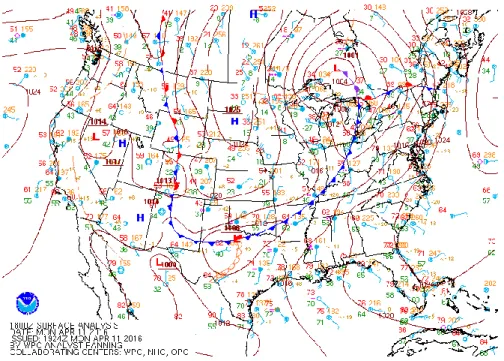
shown by solid black lines, isotherms by dashed red lines, and isodrosotherms by solid green lines. ... 36 Figure 4.5: Surface analysis from the Weather Prediction Center (WPC) valid 1800 UTC

on 11 April 2016. ... 36 Figure 4.6: Observed sounding from Fort Worth (FWD) at 1800 UTC on 11 April 2016.

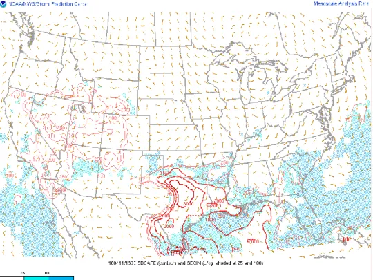
The temperature and dew point profiles are shown in red and green, respectively. Analyzed variables are derived using the NSHARP program. ... 37 Figure 4.7: Surface-based CAPE (SBCAPE; contoured) and surface-based convective

inhibition (SBCIN; shaded) at 1800 UTC on 11 April 2016. ... 38 Figure 4.8: Assimilation procedure for the experiments presented. Data assimilation

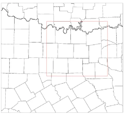
cycles begin at 2150Z, with a 1.5 hour free forecast beginning at 2220Z. Triangles represent the weighting of fractions of the computed analysis increment introduced during each assimilation window. ... 41 Figure 4.9: Model domain with the subdomain used for quantitative verification metrics

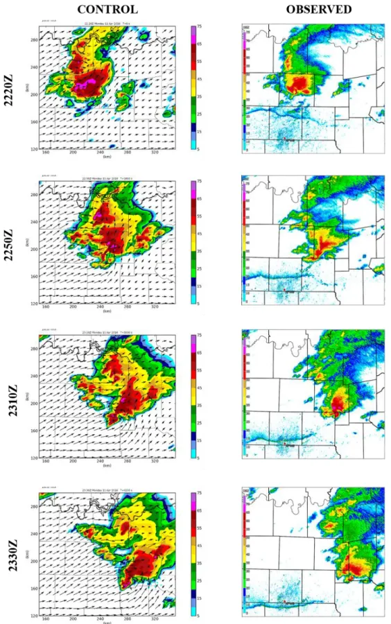
outlined in red. ... 42 Figure 4.10: Simulated reflectivity at 2 km AGL for the CONTROL experiment (left) and

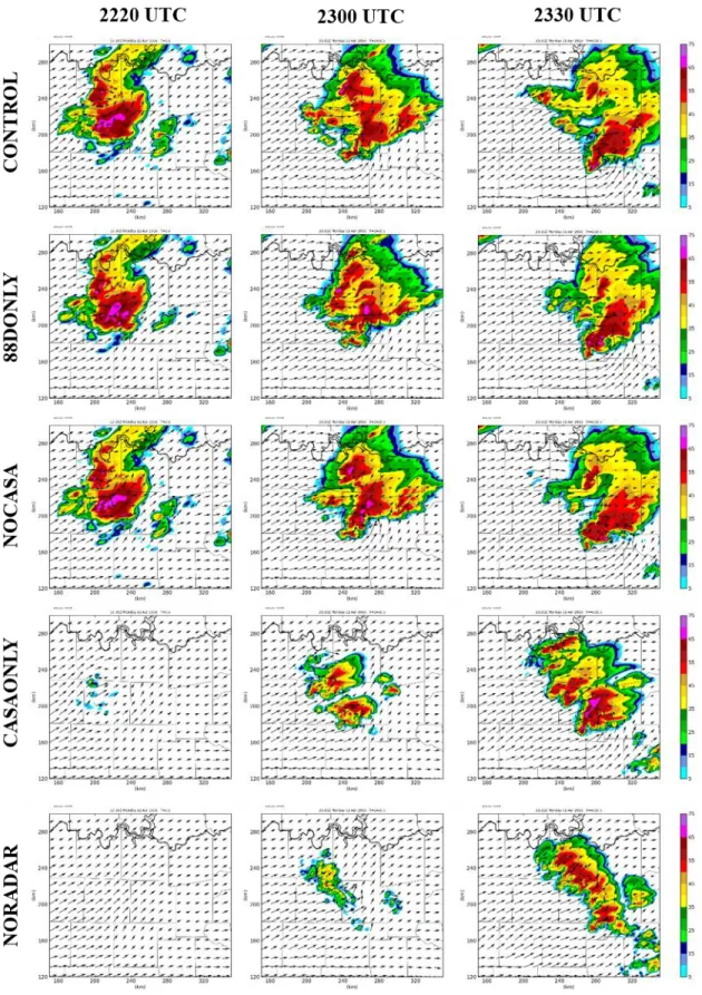
reflectivity from the KFWS 0.5 degree scan (right). ... 47 Figure 4.11: Simulated reflectivity and wind vectors at 2 km AGL for CONTROL,

(10)

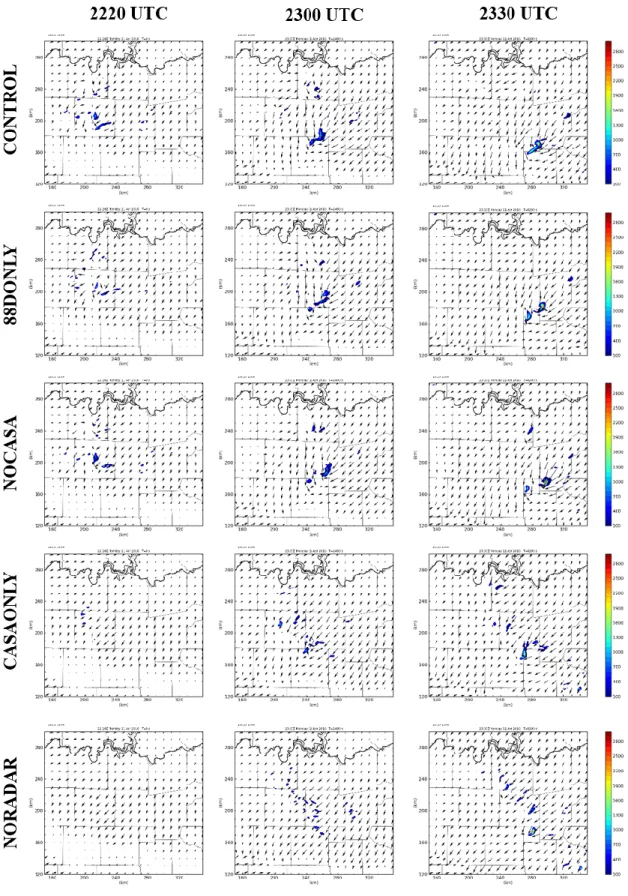
Figure 4.12: Vertical cross-sections for the CONTROL and CASAONLY experiments. ... 51 Figure 4.13: Surface winds and 1 to 5 km updraft helicity (UH) for the CONTROL,

88DONLY, NOCASA, CASAONLY, and NORADAR experiments. ... 53 Figure 4.14: Average FSS values for composite reflectivity as a function of neighborhood

size for a) 20 dBZ threshold, b) 25 dBZ threshold, and c) 30 dBZ threshold. Experiments shown include CONTROL, 88DONLY, and CASAONLY. The dashed line corresponds to the 𝐹𝑆𝑆𝑢𝑛𝑖𝑓𝑜𝑟𝑚 value. ... 56 Figure 4.15: As in Figure 4.14, but for the CONTROL, NOTESTBED, and NONEWSFC

experiments. ... 57 Figure 4.16: Time series of FSS values during the free forecast period using a 17 grid

point (16 km) neighborhood size for a) 20 dBZ, b) 25 dBZ, and c) 30 dBZ reflectivity thresholds. Experiments shown include CONTROL, 88DONLY, CASAONLY, and NORADAR. ... 59 Figure 4.17: As in Figure 4.16, but for the CONTROL, NOTESTBED, and NONEWSFC

experiments. ... 60 Figure 4.18: a) Observed MESH swath (mm) derived using WSR-88D radar data and b)

forecast MESH swath (mm) for the CONTROL experiment. MESH swaths are shown for the free forecast period, namely 2220 to 2350 UTC. ... 62 Figure 4.19: Forecast MESH swaths (mm) for the a) CONTROL, b) NORADAR, c)

88DONLY, d) NOTDWR, e) NOCASA, and f) NOCASAVR experiments. .... 65 Figure 4.20: As in Figure 4.19, but for the a) CONTROL and b) NONEWSFC

(11)

Figure 4.21: Performance diagram for radar data denial experiments, using a hail size of 5 mm and neighborhood threshold of 15 km. ... 68 Figure 4.22: As in Figure 4.21, but for a hail size of 25 mm. ... 70 Figure 4.23: As in Figure 4.22 but for surface data denial experiments. ... 71 Figure 4.24: Locations of the 10 ASOS and 2 Oklahoma Mesonet stations that are denied

for verification purposes. ... 72 Figure 4.25: Root mean square difference (RMSD) for a) 2 m temperature and b) 2 m

dew point temperature. The vertical line at 30 minutes represents the start of the free forecast. ... 74 Figure 4.26: As in Figure 4.25, but for the surface data denial experiments. ... 76 Figure 4.27: Bias for a) 2 m temperature and b) 2 m dew point temperature for the surface

data denial experiments. ... 78 Figure 4.28: Background temperature field (°C) and wind vectors (m/s) at 2150 UTC.

Independent (i.e., not assimilated) temperature and wind observations are overlaid. ... 79 Figure 4.29: Specific humidity of vapor (qv) differences at the surface, which are

determined by subtracting the qv value for the CONTROL experiment from the

value for each experiment. ... 82 Figure 4.30: Forecasted temperature (°C) and wind (m/s) fields at the surface for 2220

UTC and 2240 UTC, with observed temperature and wind fields overlaid for the 12 verification stations. ... 83 Figure 4.31: As in Figure 4.30, but for 2300 UTC and 2320 UTC. ... 84

(12)

Figure 4.32: Comparison of the reflectivity field roughly 2 km AGL for the single-moment microphysics scheme (CONTROL) and double-single-moment microphysics scheme (CTLDOUBLE). Both experiments assimilate all available data. ... 87 Figure 4.33: Forecast MESH swath (mm) for the a) CONTROL and b) CTLDOUBLE

experiments. Observed MESH above 25 mm is contoured in black. ... 88 Figure 4.34: Performance diagram comparing MESH forecasts from the CONTROL and

CTLDOUBLE experiments, using a neighborhood threshold of 15 km. ... 89 Figure 4.35: As in Figure 4.25, but for the CONTROL and CTLDOUBLE experiments. ... 90 Figure 4.36: Potential temperature perturbations at the surface, which are defined as

𝜃𝑑𝑜𝑢𝑏𝑙𝑒 − 𝜃𝑠𝑖𝑛𝑔𝑙𝑒 for a) 2220 UTC, b) 2300 UTC, and c) 2340 UTC. The reflectivity observed by the KFWS WSR-88D radar (0.5 degree tilt) at 2340 UTC is shown in d), with a fine line indicative of the placement of the cold front. ... 91 Figure A.1: Surface analysis from the Weather Prediction Center (WPC), valid at 2100

UTC on 5 November 2015. ... 115 Figure A.2: Storm Prediction Center (SPC) storm reports from 5 November 2015. Severe

hail and wind were both reported in the Dallas-Fort Worth metroplex. ... 115 Figure A.3: (Left) Outline of the geographic area considered in this study (outlined in

black), which includes Dallas-Fort Worth. (Right) The geographic location of trucks considered in this study. ... 116 Figure A.4: Results of the thinning algorithm for truck CW0WG for the time period from

1700 to 1810 UTC. The gray dots correspond to one-minute averages. A red box indicates that an experiment resulted in statistically different results. ... 116

(13)

Figure A.5: Results of the permutation test for truck CW0WG for the time period from 1700 to 1810 UTC. The rows correspond to two-minute, three-minute, four-minute, and five minute averaging windows, respectively. ... 117

(14)

Abstract

A key recommendation of a 2009 report by the National Research Council (NRC) was for new mesoscale networks to be integrated with existing ones to form a nationwide “network of networks”. This recommendation originated in response to noted deficiencies in the U.S. mesoscale observing network. The report also recommended that research testbeds be established, such as the Center for Collaborative Adaptive Sensing of the Atmosphere (CASA) DFW Urban Demonstration Network, to ascertain the potential benefit of proposed observing systems.

In this work, non-conventional surface observations from Global Science & Technology (GST) Mobile Platform Environmental Data (MoPED), WeatherBug, Citizen Weather Observer Program (CWOP), and Understory Weather in the DFW Testbed are considered. Radar data include Terminal Doppler Weather Radars (TDWRs) and CASA X-band radars. The Advanced Regional Prediction System (ARPS) model is used to perform observing system experiments (OSEs) that are designed to assess the impact of the aforementioned networks. The three-dimensional variational (3DVAR) analysis system is used, along with the complex cloud analysis, to produce analysis increments every 10 minutes, which are then applied to the model forecast using incremental analysis updating (IAU). Experiments are performed on a supercell thunderstorm that impacted the DFW metroplex on 11 April 2016 with large, damaging hail. The analysis includes qualitative and quantitative comparisons of the forecast reflectivity fields, quantitative comparisons of model-derived hail with radar-observed hail, and surface-level verification of the temperature and dew point fields. The CASA radial velocity data offer positive benefit to the forecasted storm structure as noted in the

(15)

simulated reflectivity, along with model-derived hail. However, the data appear to be detrimental when considering quantitative comparisons of the simulated reflectivity with observations. The inclusion of dew point temperature measurements from the non-conventional CWOP and WeatherBug networks resulted in a degradation in the forecasted dew point field. The analysis concludes with a brief comparison of the results for single-moment versus double-moment microphysics scheme sensitivity. Future work should assess the impacts of the non-conventional observations on a wider array of cases.

(16)

Chapter 1

1.1 A Brief History of Numerical Weather Prediction

In 1904, Norwegian meteorologist Vilhelm Bjerknes described the problem of numerical weather prediction (NWP; Bjerknes 1904). With an accurate initial depiction of the atmosphere (i.e., initial conditions), along with the corresponding boundary conditions, one should, in theory, be able to predict the future state of the atmosphere by integrating the equations of motion forward in time.

Almost two decades later in 1922, Lewis Fry Richardson proposed numerical integration as a means of forecasting the future state of the atmosphere (Richardson 1922). Integrating the primitive equations of motion by hand, Richardson predicted an inordinately large 6-hour pressure tendency of 146 hPa, a value that is unobservable in the real atmosphere. Despite the apparent failure, Richardson’s work provided the first evidence of the importance of accurately sampling the initial state of the atmosphere. The wind and pressure were out of balance owing to a scarcity of upper-air observations at the time; as such, the meteorological signal was largely masked by gravity waves attempting to restore geostrophic balance (Lynch 2008).

The combination of high-performance computing capabilities and increased surface and upper-air observations revived interest in NWP during the late 1940s (Kalnay 2003). Beginning in the 1950s, operational model forecasts have been produced by the National Center for Environmental Prediction (NCEP; formerly the National Meteorological Center, or NMC), with these forecasts becoming global in 1973. As model resolution and computing capabilities have continued to improve, the simulation of mesoscale features such as thunderstorms has become an area of research focus (Lilly

(17)

1990). However, it is widely recognized that, in order for these advances in numerical models and computing systems to be fully realized, there must be corresponding improvements in observations.

1.2 Research Motivation

In 2003, the United States Weather Research Program (USWRP) organized a workshop to discuss ways of alleviating deficiencies in the current observational network (Dabberdt et al. 2005). Although forecast skill has improved over time with improved model resolution, the full potential of advances in numerical modeling has not been realized. High spatiotemporal resolution mesoscale observations, in concert with improved data assimilation techniques and parameterization schemes, have the ability to improve forecasts of wind and precipitation. Mesoscale phenomena, such as frontal boundaries and mountain flows, along with planetary boundary layer (PBL) structures, are particularly difficult to analyze and predict with the current observational network.

The primary recommendation of the workshop was to establish a nationwide network of mesoscale surface stations that collect observations at a higher spatiotemporal resolution. These stations would complement the existing observational network by providing additional data in the lowest levels of the atmosphere where the greatest observational need exists. The committee recommended that these mesoscale surface observations be collected at least every 5 minutes and have an average station separation distance of 25 km in flat terrain. The average station separation distance should be reduced to roughly 10 km in areas of greater observational need, such as in coastal, mountainous, or urban areas.

(18)

The current Weather Surveillance Radar-1988 Doppler (WSR-88D; Crum and Alberty 1993) network of S-band (10-cm wavelength) radars is unable to observe roughly 70% of the PBL, missing important low-level features such as convective outflows and mesoscale cyclones and anticyclones. This deficiency could be remedied by integrating additional radars into the WSR-88D network, such as Terminal Doppler Weather Radars (TDWRs) and privately-owned radars operated by television stations. Furthermore, low-power, short-range radars could be strategically placed to fill in the gaps of the WSR-88D network and improve observational coverage (Dabberdt et al. 2005). This concept has been demonstrated by the Collaborative Adaptive Sensing of the Atmosphere (CASA) consortium, which installed a testbed of four X-band (3-cm wavelength) radars in southwest Oklahoma in 2006 (McLaughlin et al. 2009).

A 2009 report by the National Research Council entitled Observing Weather and Climate from the Ground up: A Nationwide Network of Networks expanded upon the findings of the 2003 workshop (National Research Council 2009). The report noted that while the United States has a respectable synoptic-scale observing network, the quantity, quality, and accessibility of mesoscale observations varies considerably, with a rather poor network of three-dimensional observations. The report proposed that existing and new mesoscale networks be integrated to form a nationwide “network of networks” in order to maximize the observational benefit of the disparate networks. These networks should include comprehensive metadata in order to maximize the value of the observations; in fact, it is recommended that complete metadata be a requirement for membership in the network of networks. The integration process should include collaboration from academic, public, and private partners, with the federal government

(19)

acting as the central authority and overseeing the resulting network. Some examples of high-priority observations include tropospheric profiles of temperature and moisture and PBL structure. An additional recommendation of the report is that the United States Department of Transportation should oversee the future deployment of high-density mobile observations, such as temperature and rain rate (from wiper speed) collected by fleets of commercial vehicles.

Testbeds have been recommended as a means of collaboration between federal, private, and academic partners (Dabberdt et al. 2005 and National Research Council 2009). These testbeds should be established in regions that present operational challenges, such as urban areas and mountainous regions, with the goal being to objectively assess the future benefit of proposed observing systems (National Research Council 2009). As detailed in Section 1.4, observing system experiments (OSEs) and observing system simulation experiments (OSSEs) can be used to objectively demonstrate whether a specific set of observations within the testbed helps improve forecast skill.

1.3 DFW Urban Demonstration Network

One such testbed has been established in the Dallas-Fort Worth (DFW) metroplex, known as the DFW Urban Demonstration Network (National Research Council 2012). The testbed is being managed by the Center for Collaborative Adaptive Sensing of the Atmosphere (CASA) and represents a joint endeavor among academic institutions, private companies, local governments, and the National Weather Service (NWS) forecast office in Fort Worth. The Dallas-Fort Worth metroplex was chosen as a suitable location for the demonstration testbed as it is a large urban area with a population in excess of 6

(20)

million people that has two major airports and several highly-traveled interstate highways. Most importantly, the region experiences a wide array of significant weather impacts, such as tornadoes, severe wind, and localized flash flooding.

A network of eight closely-spaced X-band radars is proposed to supplement the existing WSR-88D radar (KFWS) in Fort Worth by providing increased low-level coverage in regions that are poorly observed by the existing KFWS radar (McLaughlin et al. 2009). Currently, seven out of the eight planned radars have been deployed. The radar coverage in the testbed will be further supplemented by the inclusion of the TDWRs at the aforementioned passenger airports. Other data sources include satellites, radiosondes, aircraft data (e.g., take-off and landing soundings), SODARs, and various conventional and non-conventional surface observation networks. More details on the individual data sources can be found in the following chapter.

1.3.1 CASA X-band Radars

CASA, an NSF Engineering Research Center (ERC), developed and deployed a testbed of four densely-spaced X-band radars in southwest Oklahoma in 2006, known as Integrated Project One (IP1; McLaughlin et al. 2009). This region was chosen as it experiences numerous severe thunderstorms and tornadoes annually and is located roughly halfway between the existing Oklahoma City (KTLX) and Frederick (KFDR) S-band radars, resulting in poor coverage in the lowest levels of the atmosphere (Brewster et al. 2005b). Research studies that have incorporated the CASA radar data from the IP1 deployment into storm-resolving numerical models have shown positive forecast impact (Brewster et al. 2007; Schenkman et al. 2011a, b; and Snook et al. 2012). Given these promising results, a network of eight similar radars is being deployed within the DFW

(21)

Urban Demonstration Network. With continued promising results, further expansions of the X-band radar technology are certainly within the realm of possibility. These radars could either be deployed nationwide or in specified regions where there are increased observational needs, such as mountainous regions or urban areas. Roughly 10,000 radars would be required to maintain the current 30-km average separation distance in a nationwide deployment. More details on the CASA X-band radars can be found in section 2.3.

1.4 Observing System Experiments

According to Dabberdt et al. (2005), the decision-making process related to the nationwide “network of networks” should include atmospheric models, as models have the ability to quantify the greatest observational needs for analysis and prediction applications. Moreover, models are able to determine the minimum spacing and resolution requirements for NWP applications, which is important in maintaining economic viability of future nationwide observing systems. Historically, these goals have been accomplished using either observing system experiments (OSEs) or observing system simulation experiments (OSSEs). In an OSSE, the impact of proposed observing systems can be ascertained by using simulated observations. First, a high-resolution NWP model is used to generate a “nature run,” which acts as the assumed atmospheric “truth” (Atlas 1997). Simulated observations are then created from this “nature run” by, for instance, interpolating the nature run values to the observation locations. Numerical simulations using these synthetic observations are then compared to the nature run to determine the impact the proposed observations would have on numerical simulations if the system were implemented (e.g., Arnold and Dey 1986; Lord et al. 1997; Atlas 1997).

(22)

On the other hand, in an OSE, the impact of currently-deployed observing systems can be determined. Traditionally, in an OSE, an analysis and resulting forecast are computed for a control experiment in which all available real-data are assimilated. The control forecast can then be compared to data denial experiments, in which observations from a particular class of observations are denied (e.g., all aircraft observations or observations from a particular sensor type), to determine the magnitude of resulting improvements (or degradations) in the analyses and forecasts attributable to the denied dataset. It is important to note that OSEs may reveal negligible or negative value of particular observational datasets. For example, McNally et al. (2014) evaluated the impact of geostationary and polar-orbiting satellite data in the forecasted track of Hurricane Sandy, which made a sharp left turn into the coast of New Jersey in October 2012. This left hook was correctly predicted by the European Centre for Medium-Range Weather Forecasts (ECMWF) well before it was forecasted by other operational centers. The authors found that the denial of geostationary satellite data did not significantly degrade the forecasted turn; however, polar-orbiting satellite data was shown to have a more significant role in capturing the left turn in this event.

Coincident with improvements in numerical models, computational power, and data assimilation systems, increased research has been focused on determining observation impact using OSEs. These studies have considered the impact of sounding and profiler data (e.g., Graham et al. 2000; Benjamin et al. 2010; Agustí-Panareda et al. 2010), GPS-derived precipitable water (e.g., Smith et al. 2007; Benjamin et al. 2010), aircraft data (e.g., Benjamin et al. 2010), satellite radiances and satellite derived winds

(23)

(Bouttier and Kelly 2001; Zapotocny et al. 2002, 2005, 2007; Kazumori et al. 2008; Bi et al. 2011), and radar radial winds and reflectivity (Schenkman et al. 2011a,b).

Despite this upturn in OSE-related research, determining observation impact using OSEs can prove to be both time-consuming and computationally expensive, due to a large number of experiments that must be run in order to test the denial of numerous combinations of observations. In recent years, a new diagnostic tool has emerged to overcome these issues, known as Forecast Sensitivity to Observation (FSO; Cardinali 2009). In this adjoint approach, the observation impact is determined using a single experiment in which all observational data are assimilated using a four-dimensional variational (4DVAR) analysis system.

1.4.1 OSEs using Radar Data

Early efforts to determine the impact of radar data on high-resolution analyses and forecasts of convection began at the University of Oklahoma during the late 1980s and early 1990s with the inception of the Center for Analysis and Prediction of Storms (CAPS; Lilly 1990). These efforts coincided in large part with the nationwide deployment of the WSR-88D network (Crum and Alberty 1993). Assimilation of Doppler radar data is crucial for modeling ongoing thunderstorms, as Doppler radar is the only system capable of observing convective storms with the requisite spatiotemporal resolution.

It is theorized that the dense network of X-band CASA radars in the DFW Urban Demonstration Network will better observe the lowest levels of the atmosphere, filling in observation gaps in the widely-spaced WSR-88D radar network. Several studies have looked at the impact of CASA radar data from the IP1 deployment in southwest

(24)

Oklahoma during the spring of 2007. In Schenkman et al. (2011a), a tornadic mesoscale convective system (MCS) and associated line-end vortex (LEV) are simulated using the Advanced Regional Prediction System (ARPS) model. Reflectivity and radial velocity data from the WSR-88D and CASA IP1 networks are assimilated, with the ARPS 3DVAR and complex cloud analysis (Brewster et al. 2005c; Hu et al. 2006a) using these data to adjust the cloud and hydrometeor fields, along with in-cloud temperature to account for latent heating. When CASA radar data were assimilated alongside WSR-88D data, the squall line structure is improved at the end of the data assimilation window, resulting in an improved simulation. The radial velocity data from CASA were particularly important in accurately analyzing the gust front. In a closely-related study, Schenkman et al. (2011b) examined the influence of CASA radial velocity data on the prediction of tornadic mesovortices. Experiments in which low-level radial velocity data were assimilated yielded the most accurate forecast evolution, owing to improved depictions of the low-level shear profile and cold pool development. Snook et al. (2012) found that assimilating CASA and WSR-88D radar data into a forecast ensemble resulted in improved probabilistic forecasts of mesovortices, which serve as a proxy of tornado potential. Stratman and Brewster (2015) examined the influence of assimilating CASA radar data for a cluster of supercell thunderstorms on 24 May 2011 using diverse microphysics parameterization schemes. It was found that the CASA data afforded little, if any, value for a storm located outside the radar coverage area. The value added for storms inside the radar coverage area was less clear, perhaps due to the complex interactions with neighboring supercells.

(25)

Dawson and Xue (2006) demonstrated that forecasts of a strong, bow-shaped MCS most closely matched the observed system when the complex cloud analysis package was used, thus resulting in the elimination of the 2 to 3 hour model “spin-up” time. The authors also found that the use of intermittent assimilation cycles was beneficial. Hu et al. (2006a) were able to successfully reproduce a tornadic thunderstorm in the Fort Worth area, including reductions in timing and location errors, when the complex cloud analysis procedure was used in conjunction with radar reflectivity data. In addition, the model “spin-up” time was reduced with the usage of the cloud analysis package. Hu et al. (2006b) found additional forecast improvements with the assimilation of radial velocity data using the ARPS three-dimensional variational (3DVAR) data assimilation system, although a larger improvement was found with the addition of clouds and latent heat. Zhao and Xue (2009) also used the ARPS cloud analysis package to examine the impacts of reflectivity and radial velocity data from coastal WSR-88D radars on the forecasted track and intensity of landfalling Hurricane Ike in 2008. The assimilation of radial velocity data was found to be most impactful for improving the track forecast, while reflectivity data was most useful for improving the intensity forecast. Xiao and Sun (2007) found that assimilation of multiple-Doppler data resulted in improved simulations of a squall line, owing to a better initial depiction of a cold pool. Moreover, radial velocity data afforded the most benefit to wind and vertical velocity analyses, whereas radar reflectivity was most beneficial in improving hydrometeor analyses. The authors also note that cycling of the Doppler radar data results in a better analysis than when radar data is assimilated just once. Xue et al. (2013) found that assimilating radial velocity and reflectivity data from the WSR-88D network yielded a

(26)

positive impact on forecasts of convection throughout a domain covering a majority of the continental United States for a period of at least 24 hours.

It is also worth noting that improved numerical simulations of convective storms are a cornerstone of the proposed “warn-on-forecast” paradigm (Stensrud et al. 2009; Stensrud et al. 2013). In the “warn-on-forecast” paradigm, observations of convective storms and their ambient environment are assimilated into an ensemble of convection-allowing models, providing NWS forecasters and end-users with probabilistic forecast information concerning storm evolution. This information could then result in increased lead times for severe thunderstorm, tornado, and flash flood warnings, furthering the NWS mission of protecting life and property. In order for “warn-on-forecasting” to become a reality, the forecast model must accurately depict and support ongoing precipitation in the short-term forecasts. As such, continued improvements in the assimilation of radar data and other mesoscale data are necessary. To that end, this research will examine the impacts of auxiliary CASA and TDWR radar data for a case study in the DFW Urban Demonstration Network to determine if the additional data affords improved analyses and forecasts.

1.4.2 OSEs using Surface Data

As described in the previous section, numerous studies have demonstrated the value of radar data in generating useful forecasts of ongoing convection. Despite this, the use of radar data in forecasting convective initiation is fundamentally limited in that radar data only provides precipitation information and radial velocity data (i.e., no thermodynamic information is directly provided by the radar). Moreover, operationally available radar data are unable to fully observe the lowest levels of the atmosphere due

(27)

to their spacing and the Earth’s curvature. In response to this limitation, increased research focus has been placed on understanding the benefit of surface observations in relation to NWP analyses and forecasts.

Mukhopadhyay et al. (2005) utilized the Regional Atmospheric Modeling System (RAMS) to study the effect of surface observations on model forecasts of three monsoon low-pressure systems in the vicinity of India. Surface data inclusion resulted in an improved forecast of heavy rainfall throughout the region, when equitable threat score (ETS) and bias are used as forecast verification metrics. Additionally, the authors noted that the surface data appear to be particularly beneficial due to the highly-varied terrain in the region, with surface observations identifying differential heating effects. More specifically, regions of enhanced surface heating experienced a corresponding mass response of convergence and upward motion, which resulted in improved precipitation forecasts. This study underscores the need for increased density of observations in regions of complex terrain.

Alapaty et al. (2001) developed a continuous surface data assimilation technique and found that this new technique consistently improved boundary layer structure. Interestingly, the authors noted that surface data yielded the most benefit when assimilated alongside upper-level radiosonde data. In essence, the full potential of the surface data would not be realized without the additional upper-air data. One goal of this research is to identify similar relationships among observational datasets in the DFW Urban Demonstration Network in order to maximize observation benefit. In a similar study, Ha and Snyder (2014) assimilated surface observations using the Ensemble Kalman Filter (EnKF) and found improvements in subsequent Weather Research and

(28)

Forecasting (WRF) model forecasts of a squall line. Not only did the surface observations result in a better representation of the boundary layer structure, they improved horizontal gradients of both temperature and moisture that would prove crucial in properly forecasting thunderstorm development.

Knopfmeier and Stensrud (2013) compared surface analyses generated using EnKF to those produced by the NCEP’s Real-Time Mesoscale Analysis (RTMA). Surface mesonet data were assimilated in the EnKF analyses, which overall were fairly similar to the RTMA analyses, albeit with a somewhat smoother appearance. Most notably, denying up to 75% of the mesonet data resulted in only minor differences in the analyses. The authors speculate that this result is attributable to background error covariance scales that are significantly larger than the average station separation distance, thus allowing for enhanced observational increment spreading throughout the domain. This research demonstrates the value in determining optimal observational density, as suggested by Dabberdt et al. (2005).

Until recently, most studies focused on the impact of observational data have been centered on conventional observations, with only limited research focused on non-conventional datasets. Tyndall and Horel (2013) considered the impact of nearly 20,000 surface observations and found that observation impact was largely dependent on the observation location. For instance, observations located in metropolitan areas with widespread observations tended to have lower observational impact than observations in more remote locations with fewer overall observations. In addition, high-impact observations tended to be found in regions with more local variability, such as coastal regions. It is important to note that this study did not consider the impacts of observing

(29)

systems individually. Perhaps the first study to do so was Hilliker et al. (2010), which considered the impact of surface observations from Automated Weather Services, Inc. (AWS). These observations, more commonly known as “WeatherBug,” are commonly taken from the tops of buildings such as schools. The authors found improvements to National Digital Forecast Database (NDFD) forecasts of temperature and dew point. However, the observations offered limited improvements for wind speed forecasts, perhaps as a result of biases in wind speed measurements due to siting concerns (sheltering by nearby buildings and trees). NDFD forecasts use numerical model output as the starting point, but are modified by forecasters at the NWS Weather Forecast Offices (WFOs) to generate the final forecast.

More recently, Carlaw et al. (2015) examined the impact of several non-conventional data sources on ARPS forecasts of a tornadic supercell that impacted Cleburne, TX on 15 May 2013. The non-conventional surface data sources used included AWS WeatherBug, Citizen Weather Observer Program (CWOP), and Global Science and Technology (GST) Mobile Platform Environmental Data (MoPED). Given Cleburne’s location in the southwestern fringe of the DFW metroplex, it is poorly observed by conventional surface observing systems. Thermodynamic measurements from the WeatherBug stations were able to capture increased levels of moisture in the lowest levels, as compared to the model background field. Enhanced instability due to the increased humidity resulted in increases in both updraft velocity and vertical vorticity in the resultant storm, and thus produced simulated storms more closely matching observations. Carlaw (2014) examined the impacts of the aforementioned non-conventional observations on hourly analyses for a month-long period in March 2014.

(30)

Dew point errors were reduced owing to the non-conventional observations, when averaged over the entire month. Additionally, separate cases of a dryline and cold front were examined, with improvements to the analyzed boundaries in both cases. The non-conventional observations degraded the wind speed analysis, likely due to the siting issues noted in Hilliker et al. (2010).

In the framework of the nationwide “network of networks,” it is important to understand the advantages and disadvantages of various data sources in a research testbed prior to a potential nationwide deployment. The purpose of this research is to perform OSEs to determine the value of several new observing systems within the DFW Urban Demonstration Network, including non-conventional surface data and CASA radar data. Chapter 2 will describe the observational datasets used in this study, including both conventional and non-conventional observations, along with pre-processing and quality control procedures applied to these datasets. Chapter 3 will detail the ARPS model and its associated 3DVAR analysis system that are used for simulations presented in this work. Chapter 4 will present the results of OSEs performed for a high-impact hail case in the Dallas-Fort Worth metroplex on 11 April 2016. Finally, concluding remarks will be presented in Chapter 5, including implications of this work to the “network of networks” vision and suggestions for future research avenues.

(31)

Chapter 2

2.1 Conventional Observations

In this work, conventional surface data sources refer to those that are available in the federal observing network and assimilated into operational forecast models. The Automated Surface Observing System (ASOS) is one of these conventional networks, and serves as the main surface observing network in the United States (NWS 1999). The ASOS network represents a joint venture between the Federal Aviation Administration (FAA), National Weather Service (NWS), and Department of Defense (DoD), and provides valuable information for forecasting and aviation applications. The ASOS network was developed in the 1980s and deployed in the 1990s. The Automated Weather Observing System (AWOS) is a closely-related automated network that is operated by the FAA and reports data every 20 minutes at secondary airports. Sensors for both automated networks are positioned in a region that provides a representative observation for the entire airport complex (i.e., within 2 to 3 miles of the sensor location); for most airports, this location is near the touchdown zone of the main runway (NWS 1999). ASOS stations are monitored by the ASOS Operations and Monitoring Center (AOMC), with site maintenance performed by NWS technicians, as needed. Mesoscale networks (or “mesonets”) provide additional surface observations throughout the domain, and include the Oklahoma Mesonet (Brock et al. 1995; McPherson et al. 2007) and the West Texas Mesonet (Schroeder et al. 2005). In the case of the Oklahoma Mesonet, stations are sited so as ensure that the physical characteristics of a site are representative of the surrounding area (e.g., minimal terrain slope, minimal obstructions that preclude proper ventilation, and minimal influences from urban areas, forests, and bodies of water).

(32)

Sensors are calibrated prior to deployment and replaced at regular intervals, while observations are subject to automated and manual quality assurance techniques. Additional information on the Oklahoma Mesonet can be found in McPherson et al. (2007). Upper-air observations are obtained from multiple sources, including the Meteorological Data Collection and Reporting System (MDCRS), which provides observations of flight-level temperature, dew point, and wind for assimilation in forecast models. NWS radiosonde data are not available for the time period considered for this study, generally being available at 0000 and 1200 UTC, only. Data from eight radars in the WSR-88D network fall within the domain used for the 11 April 2016 case study, with the most notable being the KFWS radar in Fort Worth, Texas. Additional WSR-88D radars assimilated include Dyess Air Force Base, TX (KDYX), Frederick, OK (KFDR), Ft. Hood, TX (KGRK), Ft. Polk, LA (KPOE), Shreveport, LA (KSHV), Fort Smith, AR (KSRX), and Oklahoma City, OK (KTLX). Lastly, visible and infrared data from the Geostationary Operational Environmental Satellite (GOES) are incorporated in the complex cloud analysis, which is described in detail in Section 3.2.2.

2.2 Non-Conventional Observations

With the inception of the National Mesonet Pilot Program, Global Science & Technology (GST) was selected to develop a new system known as Mobile Platform Environmental Data (MoPED), collecting observations from sensors developed by Weather Telematics and mounted on mobile fleets of trucks and other transportation vehicles (Dahlia 2013). Since its beginning, MoPED has rapidly grown to provide more than two million observations daily, with the majority of observations originating from a fleet of over 1500 Con-way freight trucks. These trucks have been fitted with sensors

(33)

that measure such variables as temperature, humidity, pressure, and precipitation. One limitation of the MoPED system is that wind cannot be measured due to contamination from the motion of the vehicles. Pressure measurements are corrected to account for these effects. Since active vehicles collect data roughly every ten seconds, a data thinning algorithm has been developed to reduce the spatiotemporal resolution of these data. Observations are grouped together based upon truck identifier and thinned once either a five-minute time threshold or a one kilometer distance threshold are met. Appendix A presents the results of statistical testing for various averaging schemes that only considered the effects of time, with these results helping motivate the final thinning methodology.

The Automatic Position Reporting System as a Weather Network (APRSWXNET) represents an additional non-conventional data source in the DFW Urban Demonstration Network (CWOP 2014). Electronic weather stations owned by ham radio operators and private citizens collect weather observations, which are ingested into the Meteorological Assimilation Data Ingest System (MADIS). These observations are subjected to the MADIS Quality Control and Monitoring System (QCMS), which performs a variety of quality control checks. This data source is more commonly known as the Citizen Weather Observer Program (CWOP).

A third non-conventional data source is the Automated Weather Services (AWS) Convergence Technologies, Inc. WeatherBug network, which is operated by Earth Networks. There are roughly 8,000 WeatherBug weather stations throughout the United States, the majority of which are located atop schools and public buildings. These data are used daily in local weather broadcasts owing to partnerships with over 100 television

(34)

stations. Additionally, educational tools utilizing these data are made available to K-12 school children. The expansive network of WeatherBug observations offers the potential for improvements to NWP forecasts, which has been demonstrated in Hilliker et al. (2010) and Carlaw et al. (2015).

A recently deployed network of solar-powered weather stations from Understory Weather represents the fourth non-conventional data source. This dense network was originally focused on the immediate Dallas area, with ten stations deployed at the time of the 11 April 2016 case study. Since this time, the number of deployed stations has increased considerably, including increases in spatial coverage, with the full network of about 120 stations largely in place by April 2017. Temperature, pressure and humidity variables are measured using standard sensors, while wind, rain, and hail impacts are calculated based upon the forces acting on a metallic ball, or sonde. While these data are mainly intended for insurance companies responding to weather-related insurance claims, they could offer improvements to NWP forecast models.

It is important to note that these non-conventional surface data sources are not subjected to the same siting standards as the ASOS and AWOS networks. Thus, these data may be subject to bias and representativeness errors, such as the low wind speed bias noted previously by Hilliker et al. (2010) and Carlaw et al. (2015).

Since the NWS radiosonde network typically only samples the vertical profiles of wind, temperature, and dew point at 12 hour intervals, additional instruments can be used to provide more continuous coverage of vertical profiles. For instance, two SecondWind (now part of Vaisala) SODARs (SOnic Detection And Ranging) have been installed by WeatherFlow in the DFW Urban Demonstration Network to fill in these temporal gaps,

(35)

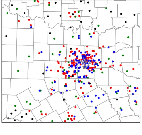
one at the Fort Worth NWS forecast office and the other in Midlothian. Wind speed and direction in the PBL (up to about 2 km) are derived from these ground-based remote sensing instruments by measuring the Doppler shift of acoustic sinusoidal pulses that are scattered back by turbulence resulting from the atmosphere’s thermodynamic structure (Lang and McKeogh 2011). Figure 2.1 displays a typical distribution of both conventional and non-conventional surface data sources, along with the locations of two SODARS, in the DFW Urban Demonstration Network. The impact of the non-conventional surface observations on analyses and forecasts will be examined in this study.

Figure 2.1: Spatial distribution of the conventional and non-conventional surface data assimilated at the first analysis time (2150 UTC). Observations shown include CWOP (red – 148), METAR (green – 44), WeatherBug (blue – 105), Understory (gray – 10), mesonet (black – 32), and SODAR (teal triangles – 2).

(36)

2.3 Non-Conventional Radar Data

The CASA Integrated Project One (IP1) testbed from the spring of 2007 consisted of four dual-polarization X-band Doppler radars located in southwest Oklahoma, a region susceptible to severe thunderstorms (McLaughlin et al. 2009). The radars were spaced 30 km apart, on average, and have a range of 40 km. These radars have a wavelength of 3.2 cm, requiring an antenna size of roughly 1 m, significantly smaller than the 8.5 m antennas required for the 10-cm WSR-88D radars. This allows the radar antennas to be placed on existing infrastructure, such as cell towers and buildings. The short wavelength, however, makes these X-band radars susceptible to attenuation in regions where the radar reflectivity factor exceeds 40 dBZ (Brewster et al. 2005a). Thus, these radar networks are designed to provide overlapping radar coverage, whenever possible (Brewster et al. 2005b). In recent years, the CASA testbed has been relocated to the Dallas-Fort Worth metroplex, with radars located in Addison, Arlington, Denton, Midlothian, Fort Worth, and Johnson County at the time of the 11 April 2016 case study. Since this time, an additional radar has been deployed in Mesquite, with a further radar planned for McKinney (Brewster et al. 2017). This network is comprised of the four radars from the original IP1 network, along with additional radars from EWR Weather Radar, Ridgeline Instruments, Furuno, and Enterprise Electronics Corporation. This network is the result of a multisector partnership between CASA and the North Central Texas Council of Governments (NCTCOG; Bajaj and Philips 2012). The beam width for each of the CASA X-band radars used in this work is shown in Table 2.1.

(37)

Table 2.1: Beam Width for CASA X-band Radars

Radar Beam Width

Addison (XADD) 2.3 degrees

Arlington (XUTA) 1.8 degrees

Denton (XUNT) 2.7 degrees

Fort Worth (XFTW) 1.8 degrees

Johnson County (XJCO) 1.8 degrees

Midlothian (XMDL) 1.4 degrees

One of the more notable features of the CASA IP1 radar network is the ability to scan the atmosphere both collaboratively and adaptively. Collaborative sensing occurs when the radar control architecture from multiple radars coordinate with one another to observe the same volume simultaneously, which allows for radar-based detection algorithms such as multiple-Doppler wind retrievals. Scanning strategies of the radars can also be modified by the radar control architecture based on the current highest priority observational needs, referred to as adaptive sensing. Together, these features allow the radars to provide improved horizontal resolution and faster update times. One example of a meteorological phenomenon in which these adaptive scanning strategies would prove useful is a supercell thunderstorm with rapidly evolving low-level rotation. Rapidly forming and dissipating tornadic signatures could be observed by the X-band radars, but be missed if they occurred between scans of the WSR-88D or below the lowest elevation scan in the low-level data coverage gap. To date, these collaborative adaptive scanning strategies have not been implemented in the Dallas-Fort Worth testbed. Rather, the radars follow a traditional “sit-and-spin” scanning strategy, with pre-determined scanning

(38)

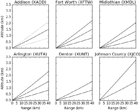
angles (see Figure 2.2) concentrating on low-level scans. Despite this, these radars afford improved spatial coverage and faster update times than the existing WSR-88D network.

In addition, two Terminal Doppler Weather Radars (TDWRs) are available from the two major passenger airports in the DFW metroplex (Istok et al. 2008). These C-band (5-cm wavelength) radars are operated by the FAA. There are 45 TDWRs operational at selected airports, with these radars mainly designed for the detection of precipitation and hazardous wind shear near airports. Figure 2.3 displays the spatial distribution of the WSR-88D radars used in this study, while Figure 2.4 displays the spatial distribution of the two TDWR and six CASA radars deployed as of 11 April 2016, with the locations of the as yet deployed McKinney and Mesquite radars shown, as well.

Figure 2.2: Radar beam heights vs. range for the six CASA X-band radars used in this study. Beam spreading is illustrated in the upper left panel for the Addison radar, using a representative beam width of 1.8 degrees.

(39)

Figure 2.3: Locations of the 8 WSR-88D radars whose data are used in this work. The blue shaded region represents the model domain used.

Figure 2.4: Locations of the radars used in this study. CASA X-band range rings are shown in blue (active for this case study) and green (proposed), TDWR range rings are shown in red, and the WSR-88D KFWS range ring is in black. The range rings for seven

(40)

2.4 Quality Control Procedures

Observations assimilated in this work are subject to several quality control procedures. Observations acquired from MADIS undergo internal quality control checks, the details of which are outlined in the NWS Techniques Specification Package (NWS 1994). Radar data are also subject to quality control procedures in the ARPS radar remapping program, which is described in the following chapter.

Furthermore, the ARPS 3DVAR analysis program also employs several quality control checks to remove inaccurate observations. Observations undergo a temporal consistency check, which compares each observation to a preceding observation at the same location, typically one hour earlier. When the difference in these observations exceeds a user-defined difference threshold, the observation is deemed to be unreliable and is not assimilated. Similarly, observations are discarded when the difference between the observed value and the background value interpolated to the observation location via the forward operator exceeds a user-defined threshold. Finally, a local Barnes (Barnes 1964) analysis to each observation site is used to check for spatial consistency among nearby observations.

(41)

Chapter 3

3.1 Advanced Regional Prediction System (ARPS)

The Center for Analysis and Prediction of Storms (CAPS) at the University of Oklahoma developed the first version of the Advanced Regional Prediction System (ARPS) model during the early 1990s (Xue et al. 1995, 2000, 2001). ARPS is a compressible, non-hydrostatic model with a terrain-following vertical coordinate on an Arakawa C-grid. The vertical coordinate is stretched using a hyperbolic tangent function. Simulations of tropical cyclones (Zhao and Xue 2009), MCSs (Dawson and Xue 2006) and tornadoes (Xue et al. 2014) have been performed using ARPS. The ARPS model is used to perform the OSEs presented in this research. Details on the parameterization schemes and model configurations used in these experiments can be found in Table 3.1.

Table 3.1: Model parameterizations and configurations

Microphysics Single-Moment (Milbrandt and Yau 2005)

Radiation NASA atmospheric radiation transfer

Planetary Boundary Layer (PBL) 1.5 order TKE (Deardorff 1980)

Advection Fourth-order in the vertical and horizontal

Convection Explicitly resolved

Soil Model Two-layer diffusive soil model (Noilhan and Planton 1989)

3.2 ARPS Three-Dimensional Variational (3DVAR) Analysis System

The ARPS three-dimensional variational (3DVAR; Gao et al. 2004) analysis system produces an analysis by combining information from the background field and

(42)

observations. The analysis is found by minimizing a scalar cost function, which is given by:

𝐽(𝑥) =1₂(𝑥 − 𝑥𝑏)T𝐁−1(𝑥 − 𝑥𝑏) +1₂(𝐻(𝑥) − 𝑦𝑜)T𝐑−1(𝐻(𝑥) − 𝑦𝑜) + 𝐽𝑐 (3.1) The first term on the right hand side measures the distance between the analysis of the state variable, x, and the background field, 𝑥_𝑏, and is weighted by the inverse of the background error covariance matrix, B. The second term represents the distance between the analysis, x, brought to observation locations by the forward operator, H, and the observed variables, 𝑦_𝑜, and is weighted by the inverse of the observation error covariance matrix, R. Cross-correlations between model variables are not included in the B matrix, and a first-order recursive filter (Hayden and Purser 1995) is used to generate the isotropic Gaussian spatial error correlations. Furthermore, observational errors are assumed to be uncorrelated, resulting in a diagonal observation error covariance matrix.

The final term in equation (3.1) is a penalty term, and represents a weak anelastic mass continuity constraint:

𝐽_𝑐 =1₂𝜆_𝑐𝐷2 _(3.2)

where D is given by:

𝐷 = 𝛼 (𝜕𝜌_𝜕𝑥̅𝑢+𝜕𝜌_𝜕𝑦̅𝑣) + 𝛽 (𝜕𝜌_𝜕𝑧̅𝑤) (3.3) Here, 𝜆𝑐 represents a weighting coefficient for the mass continuity constraint, 𝛼 and 𝛽 correspond to weighting terms for the horizontal and vertical terms, respectively, and 𝜌̅ is the mean air density at a given height. The anelastic mass continuity constraint acts to derive non-radial wind information from the observed radial velocities (Gao et al. 2004; Hu et al. 2006b). It is a weak constraint, meaning that the mass divergence does not have

(43)

vertical grid spacing are nearly the same), the anelastic mass divergence constraint is found to result in accurate analyses of vertical and horizontal velocity (Hu et al. 2006b). However, when the horizontal grid spacing is much larger than the vertical grid spacing (i.e., the aspect ratio is over 100), which is often true in the lowest levels of the model, adjustments to the vertical velocity dominate adjustments to the horizontal component of the wind. This work follows that of Carlaw et al. (2015), which uses a horizontal weighting coefficient (𝛼) that is an order of magnitude larger than the vertical weighting coefficient (𝛽).

The ARPS 3DVAR system numerically minimizes an incremental form of the 3DVAR cost function using a conjugate-gradient minimization algorithm. Furthermore, preconditioning is used to reduce the computational cost by reducing the number of iterations necessary for the minimization algorithm to converge to the final analysis. More information on the ARPS 3DVAR analysis system can be found in Gao et al. (2004).

3.2.1 Incremental Analysis Updating

When numerical models are forced to adjust to large volumes of information, all applied at the initial time, nonphysical adjustment processes such as gravity waves (or noise) often occur (e.g., Bloom et al. 1996; Brewster 2003). To combat this issue, this research utilizes Incremental Analysis Updating (IAU), which is a method that applies analysis increments computed at the initial time gradually as a constant forcing for the model throughout an integration period (Bloom et al. 1996). The general procedure of IAU is to apply the analysis increments during the model’s large time-step after all of the other forcing terms have been applied. The analysis increments are generally applied

(44)

using a triangular distribution in time, thus applying the largest portion of the observation increment during the middle of the time window. Increments are generally not applied to the pressure and vertical velocity fields during IAU at storm-scales, as these fields are not well observed and rapidly respond to changes in other model fields. Recently, the ARPS IAU code has been updated to allow users to specify more than one shape for IAU to make the distribution in time different for each variable (Brewster et al. 2015). More specifically, one can apply a larger portion of the wind and latent heat increments at the start of the assimilation window, while applying a more significant portion of the hydrometeor increments at the end of the window. This has been shown to mitigate difficulties maintaining an updraft in a convective system by allowing some time for the model to establish wind and mass fields that are capable of supporting the weight of precipitation species before introducing additional precipitation.

Additional information on the ARPS IAU with variable dependent timing (IAU-VDT) can be found in Brewster et al. (2015), while the theoretical basis can be found in Bloom et al. (1996).

3.2.2 Complex Cloud Analysis

The variational assimilation of radar reflectivity data is rather challenging owing to nonlinearities in the microphysical models and complex cross-correlations among variables. To account for these issues, the ARPS complex cloud analysis package is used in lieu of variational assimilation to account for radar reflectivity data (Brewster et al. 2005c; Hu et al. 2006a). The cloud analysis procedure uses satellite, radar, and surface observations of cloud layers to modify hydrometeor fields by using equations that relate hydrometeor mixing ratio values and observed radar reflectivity (e.g., Ferrier 1994;

(45)

Rogers and Yau 1989), recently updated to allow inversion of hydrometeor-to-reflectivity equations for all the microphysics schemes used in ARPS and WRF (Brewster and Stratman 2015). The complex cloud analysis is performed after the 3DVAR minimization is completed.

The background hydrometeor mixing ratio values are replaced by reflectivity-derived values in regions where radar reflectivity is above a user-defined threshold (typically 10 to 20 dBZ). This is based upon the belief that at this scale the radar observations, after quality control to remove non-precipitation echoes, are superior to the model background field. On the other hand, precipitation in the model background field is removed in regions where there is radar coverage and radar reflectivity is below the prescribed threshold, thus removing spurious convection from the model field. Finally, the cloud analysis procedure adjusts the temperature profile in regions where clouds and updrafts are present to account for the latent heat released during condensation processes. This has been shown to be important in maintaining updrafts in non-hydrostatic models, such as ARPS. To calculate the temperature adjustment due to latent heating, a moist adiabatic ascent is calculated from the cloud-base, with entrainment in areas of analyzed ascent, and the resulting temperature values replacing the 3DVAR analysis value in regions where the analyzed temperature is colder. More details on the complex cloud analysis procedure can be found in Brewster et al. (2005c) and Hu et al. (2006a).

3.2.3 Radar Remapping

Prior to being utilized in 3DVAR or the complex cloud analysis package, radar data must first be quality-controlled to account for radar artifacts. First, the raw radar data are checked for beam blockage effects (e.g., from tall buildings and trees) and sun

(46)

strobes during sunrise and sunset. Then, the raw radar data are checked for anomalous propagation effects, in which the radar beam is refracted towards the earth’s surface, by identifying regions of large vertical reflectivity gradients, reflectivity texture, and low radial velocities. Isolated non-meteorological echoes are removed using a “despleckling” algorithm. Finally, the raw radar data are checked for velocity aliasing. This is performed by first converting the radial velocity data into increments from the mean wind, where the mean wind field represents an average of nearby data points in the background wind field. This mitigates effects of the vertical shear of the mean wind and helps pinpoint isolated regions of aliased velocities. Horizontal consistency checks are then performed across neighboring radials by calculating gate-to-gate shear; this is applied to the perturbation radial velocities following the method described in Eilts and Smith (1990). Once all of the quality checks are performed, the radar data are remapped from the polar coordinate system to the Cartesian grid used by ARPS via a least squares fit to a quadratic function in the horizontal and to a linear function in the vertical. In addition to reflectivity and radial velocity data, the remapping program has the capability of producing velocity azimuth display (VAD) wind profiles. Additional details concerning the ARPS radar remapping algorithm are found in Brewster et al. (2005c).

(47)

Chapter 4

4.1 Case Study

During the afternoon and early evening hours of 11 April 2016, a prolific hail-producing supercell thunderstorm affected north-central Texas, including the northern portion of the Dallas-Fort Worth metropolitan area. The supercell thunderstorm formed around 1900 UTC (2:00 PM CDT) just southwest of Wichita Falls and quickly became severe as it tracked to the east-southeast.

Severe storm reports from the Storm Prediction Center (SPC) are shown in Figure 4.1a, with numerous significant severe hail reports (diameter in excess of 2 inches, 5 cm) occurring along the track of this storm. Figure 4.1b zooms in on the severe storm reports occurring in the northern portion of the Fort Worth NWS forecast office’s area of responsibility. The first significant severe hail report occurred around 2000 UTC in Archer County, just south of Wichita Falls. Significant severe hail was reported in Wise County, Texas beginning around 2130 UTC. The storm continued into Denton County around 2210 UTC, with grapefruit sized hail (4.00 inch diameter, 10 cm) reported around 2220 UTC. Significant severe hail also occurred in Plano, Allen, and Wylie in Collin County, with an additional report of grapefruit sized hail occurring in Rockwall County around 2310 UTC. The largest hail associated with the storm was reported in Wylie, with 5.25 inch (13.3 cm) diameter hail reported. The storm then gradually weakened as it moved out of the metropolitan area. This hail storm, in conjunction with a separate storm in San Antonio, Texas the following day resulted in an estimated total of $3.5 billion in damage (NOAA 2017).

(48)

Figure 4.1: (a) Storm Prediction Center (SPC) severe storm reports for 11 April 2016 and (b) zoomed in severe storm reports for the storm of interest. Image credit: NWS Fort Worth, Texas (obtained online at http://www.weather.gov/fwd/20160411).

4.1.1 Synoptic Setup

A shortwave trough was present over the southern Plains, extending from the Texas Panhandle through New Mexico at 1200 UTC on 11 April 2016, as shown in the 500-mb upper-air chart (Figure 4.2). This trough deepened and moved to the east during the day, with a region of differential cyclonic vorticity advection (DCVA) present

(49)

downstream of the trough axis. In addition, a region of upper-level divergence is evident in the 300-mb chart, in response to the incoming subtropical jet stream maximum (Figure 4.3). Together, these features resulted in the development of a surface low pressure system, centered over northwest Texas. Southerly winds in the low-levels, as seen in the 925-mb analysis (Figure 4.4), afforded a rich moisture return, which, along with mid-level westerly winds, allowed for the formation of a dryline (e.g., Schaefer 1974; McCarthy and Koch 1982).

By 1800 UTC, the surface low pressure system was centered over northwestern Texas, just south of Wichita Falls (Figure 4.5). The aforementioned dryline extended south from this low pressure system through the Hill Country and Big Bend Regions of Texas. A cold front was present just south of Wichita Falls, Texas, with a cold front extending west from the low pressure system into New Mexico. A surface low pressure system centered north of the Great Lakes was associated with an additional cold front, which extended southwest to the Red River.

(50)

Figure 4.2: 500-mb upper-air analysis valid 1200 UTC on 11 April 2016. Solid black lines represent geopotential height contours (isohypses), while dashed red lines are isotherms.

Figure 4.3: 300-mb upper-air analysis valid 1200 UTC on 11 April 2016. Isotachs are shaded, while streamlines are represented by solid arrows, and divergence is shown by solid yellow lines.