1
Performance Drivers in Private Infrastructure Funds
Martin Haran1, Daniel Lo2 and Stanimira Milcheva3
Abstract
Research on infrastructure as an asset class is still in its infancy due to the lack of data. Investors have approached the performance evaluation of infrastructure deals from the lens of either real estate or private equity. We use fund-level cash flow data to construct three performance metrics: the internal rate of return (IRR), the public market equivalent (PME) and the total value to paid-in capital (TVPI) and assess the performance drivers of private infrastructure funds. Our results highlight that private infrastructure funds exhibit a different performance pattern to mainstream private equity funds and to real estate private equity. Performance determinants such as fund size, investment style, fund specialisation, sector, location do not seem to explain the cross-section in performance indicators. All else equal, oversubscribed funds deliver a worse performance. Results for persistence across follow-on funds are inconclusive and we find mild momentum effects. Our results have implications for investors in real assets and less transparent markets. Overall, the private infrastructure fund sector is still in its infancy and conventional wisdom from general private equity or real estate research may not yet apply to infrastructure funds.
Keywords: Private infrastructure funds, performance, persistence, internal rate of return, public market equivalent.
1Ulster University, Jordanstown Campus, Shore Road, Newtownabbey, BT37 0QB, email: [email protected] 2 Ulster University, Jordanstown Campus, Shore Road, Newtownabbey, BT37 0QB, email: [email protected] 3 University College London, Bartlett Faculty of Built Environment, 1-19 Torrington Place, London WC1E 7HB, email: [email protected]
2
1 Introduction
The role of the private sector in the provision and financing of infrastructure projects has grown markedly over the course of the last decade culminating in infrastructure assuming an increasingly prominent position within the alternative investment universe. The scale and magnitude of the infrastructure investment need4 allied with deficiencies in public sector
capacity have created a platform for increased private sector provision of infrastructure. Characteristics of some infrastructure assets such as long maturities and stable returns (for regulated industries) has served as the key drivers to the pronounced increase in the volumes of private capital which has flowed into the infrastructure sector (Gatti, 2014). Indeed, after the Global Financial Crisis (GFC), institutional investors ‘search for yield’ – beyond the conventional mainstream investment asset classes – ensured infrastructure assumed increased prominence as a desirable alternative investment option (Gatti and Della Croce 2015).
Notably, about 10% of global infrastructure investment in the last decade has been conducted via private infrastructure funds, with the Preqin infrastructure funds universe detailing that private funds held $582 billion assets under management as at the end of June 2019 (Preqin, 2020). Further exploration of the Preqin data reveals that the period between 2005 and 2019 has seen a total of 946 funds achieve financial close with combined capital raised of $675 billion. While the private equity infrastructure fund market remains comparatively small in overall value terms ($582bn) relative to the mainstream private equity funds market ($4,106bn) and the real estate private equity fund sector ($992bn)5, its growth over the last
decade has been unprecedented. The sector has grown five–fold in terms of assets under management (AUM) within the last ten years, partially due to the interest by new types of investors (Haran et al., 2020).
Evaluating the performance of infrastructure assets in general has been challenging and some initial attempts have been made by researchers (see Blanc-Brude (2014), Blanc-Brude and Hasan (2016), Blanc-Brude et. al. (2017, 2018), Andonov et al. (2019)). However, academic
4 Research by the McKinsey Global Institute (2017) estimate infrastructure investment need at $3.3 trillion annually through to 2030 – premised on current levels of investment this constitutes a shortfall $350 billion per annum.
3
research on infrastructure assets has been sparse compared to other real assets such as real estate. This is mostly due to data limitations and is especially true for private infrastructure funds instead of the listed side of the market. In general, it is hard to compare infrastructure performance on a like-for-like basis due to the lack of clear and agreed international performance benchmarks in tandem with the paucity of high-quality historical data (Cusumano et al. 2018).
The lack of reliable data and the relative immaturity of the infrastructure asset class mean that many investors have often considered investing in infrastructure as part of their real estate portfolio with the term ‘real assets’ being used as an umbrella reference to encompass both real estate and infrastructure investments. Infrastructure assets have indeed a number of similarities with real estate assets. They are both heavily capital intensive with infrastructure being even more capital intensive than real estate. As a result of that, both asset types face major illiquidity problems which is also something that characterises the wider private equity market more generally. Infrastructure assets are also highly heterogeneous and grouped into sub-sectors, similar to real estate. Investment styles across the funds universe also follow broadly similar categories as real estate with core funds at the lower end of the risk spectrum while funds pursing an opportunistic investment strategy pursue the riskiest investments. Similar to the direct and unlisted real estate markets, the infrastructure equivalents are also characterised by low transparency. Access to data for the private infrastructure markets is even harder as compared to the real estate market.
On the other hand, the performance characteristics of infrastructure have been compared to those in private equity funds. Despite the sustained growth in the infrastructure private funds universe and unprecedented volumes of capital that has been committed to the sector in the post-GFC period, there is almost no academic research on the financial and investment performance of infrastructure funds. To our knowledge, there is only one paper that assesses the performance on infrastructure funds. A seminal study by Andonov et al. (2019) evaluated infrastructure fund performance relative to the wider private equity funds universe. Their research finds that the cash flows delivered by private infrastructure funds display similar volatility and cyclicality to the wider private equity market. Their findings also infer that public investors including pension funds had heightened levels of exposure to underperforming
4
infrastructure funds something they claim has resulted in an implicit public sector subsidy of over $2 billion per year to infrastructure as an asset class.
The aim of this paper is to address the lack of empirical research on the performance drivers of infrastructure funds and to widen the debate on what private infrastructure funds as a sub-sector within the infrastructure asset class offer prospective investors. We also draw conclusions on how performance of infrastructure funds compares to general private equity and real estate funds.
We follow the seminal work by Kaplan and Schoar (2005), who are among the first to analyse the performance and persistence of private equity funds. We assess drivers of performance and explore if there is persistence for infrastructure funds over time and in the cross-section. We use classic private equity performance metrics including the internal rate of return (IRR), and multiples such as the Total Value to Paid-In Capital (TVPI). We construct our own measures of performance using cash flow data from Preqin in addition to reported metrics by general partners (GPs) or/and limited partners (LPs). Preqin is one of the main providers of data on private funds and has been used in recent research on private equity and infrastructure funds. We use two sets of data: reported performance which is available at the cross-section only and fund-level performance over time based on cash flow data. We assess performance by analysing (1) the drivers of the internal rate of return (IRR), the public market equivalent (PME) and the total value to paid-in (TVPI) and (2) the persistence of performance across follow-on funds of the same family.
Fund persistence is a key constituent of the infrastructure funds universe. In what has become an increasingly ‘crowded and competitive market’ funds seeking to raise capital for succession funds point to the performance of previous funds as endorsement of their credentials to effectively deploy capital and deliver upon investor expectations. In many cases however the funds utilised as ‘exemplars’ of performance have not fully liquidated. While there is no robust academic evidence to suggest performance manipulation research on the mainstream private equity fund market, Brown et al. (2019) find abnormal returns reported during the fund-raising cycle of a succession fund are typically lower after the subsequent fundraising cycle concludes. Infrastructure investors in the last 3-4 years have increasingly been drawn towards fund management houses with ‘proven’ performance track records. Indeed, many of the succession funds of ‘established’ infrastructure fund management houses routinely exceed their capital raising targets. By contrast less established fund managers are spending
5
increasingly longer capital raising as investor due diligence appears to have ramped up to coincide with the first phase of post-GFC infrastructure fund liquidations (Haran et al, 2020). While most of those funds are not yet liquidated thus making it hard to compare with findings from private equity literature, our results highlight that private infrastructure funds exhibit a different performance pattern to mainstream private equity funds and to direct real estate. Performance determinants such as fund size, investment style, fund specialisation, sector, location do not seem to explain the cross-section in performance indicators. We find instead that fund managers do not learn from past experience and predecessor funds with high levels of dry powder are followed by funds with even more dry powder. There is also some evidence for funds that perform well to be followed by funds that perform worse. Momentum effects over time are also found. Overall, the private infrastructure fund sector is still in its infancy and conventional wisdom from general private equity or real estate research may not yet apply to infrastructure funds.
The remainder of the paper is structured as follows. Section 2 comprises the literature review. Section 3 provides context about infrastructure private equity funds. Section 4 provides the methodology. Section 5 affords an overview of the data. The results are presented in Section 6. Section 7 concludes.
2 Private equity literature on persistence
Kaplan and Schoar (2005) are among the first to assess the performance persistence of private equity funds. Those private equity funds include mostly Venture Capital (VC) and leveraged buyouts (LBO). The authors find that returns persist strongly across subsequent funds of the same fund management company with better performing funds more likely to raise a follow-on fund. By way of cfollow-ontrast, Phalippou (2010) finds that performance persistence of VC funds is primarily concentrated within underperforming funds. Chung (2012) uses Preqin data to also explore persistence for private equity and VC funds. His results show performance persistence to be a short-term phenomenon, primarily observed in consecutive funds. Korteweg and Sorensen (2017) meanwhile found that long-term persistence has declined in the 2000s relative to the 1990s. They detail that the decline in performance persistence is largest for venture capital firms. Consistent with the findings of Harris et al. (2014) the authors
6
find substantial persistence still exists for BO and other firms post-2000. In the case of buyout funds persistence is concentrated in the lower end of the performance distribution.
Korteweg and Sorensen (2017) furthered the analysis of performance persistence by differentiating between three different forms of persistence from the investor perspective. First, they define ‘long-term persistence’ as the possibility that some private equity firms generate consistently higher (or lower) expected returns (net of fees). LPs can outperform by investing in these skilled firms with high expected returns. Second, ‘investable persistence’
reflects the difficulty of identifying the funds with high expected returns. When performance is noisy, top quartile past performance could be due to luck and does not necessarily predict future top quartile performance. The third component, ‘spurious persistence’, arises from the partial overlap of consecutive funds that are managed by the same PE firm. Partially overlapping funds are exposed to the same market conditions during the overlap period and thus induce a positive correlation in the performance of subsequent overlapping funds. Meanwhile, Braun et al. (2017) also highlight the presence of spurious patterns persistence in instances where assets are ‘rolled over’ into successor funds. This could in theory be more pertinent within the infrastructure private equity firms – particularly in the case of greenfield assets which have not fully matured.
The literature on performance persistence details the intrinsic link between the role of the fund manager and the investment decision making process in private equity. Kandel et al. (2011) and Ewens et al. (2013) argue that the defined life of private equity funds can lead GPs to make inefficient investments in risky projects. Axelson et al. (2009) also highlight that the fixed investment period of private equity funds results in incentives for the GPs to ‘burn money’ at the end of the investment period. GPs with unspent capital near the end of the investment period face a dilemma. If they do not invest, they forgo fees on the unallocated portion of the committed capital. If they invest, they earn these fees. Moreover, raising a follow-on fund is harder if the GP still has a lot of unspent capital in an existing fund (Hochberg et al., 2014). Thus, towards the end of the investment period the GP has a dual incentive to invest even if the deals that are not always in the best interest of the LPs (Axelson et al., 2009). Van der Spek (2017) showed using simulation analysis that closed-ended real estate value add and opportunistic funds have total fee leakage of approximately 2.6–3.3% per annum.
7
Research by Haran et al. (2020) highlights what could be construed as ‘irrational’ patterns of behaviour within the private infrastructure fund market over the course of the last five years. Such behavioural traits are consistent with previous research depicting (1) incentive bias which serves to benefit fund managers rather than investors with growing fees at the expense of returns (Harris et al. 2014; Kaplan and Schoar, 2005; Robinson and Sensoy, 2013); investing at market peaks when expected returns are modest (Axelson et al., 2009 and Jenkinson et al. 2013), and exiting transactions prematurely to facilitate fundraising (Gompers and Lerner, 2000). The performance credentials and track record of a fund manager nonetheless remain an important factor in the investment decision. Indeed, Aarts and Baum (2016) in their study of performance persistent of private equity real estate funds highlight past performance and length of track record of the fund manager as the key determinants in the decision to invest – as such there is an implicit assumption on the part of investors that past performance is an indicator of future performance. In other words, investors implicitly assume performance persistence.
Despite this overriding assumption, there has been to date very limited research on performance persistence of private equity funds investing in real assets (real estate/infrastructure). Hahn et al. (2005) were the first to investigate performance persistence across real estate private equity funds. Using Pension Consulting Alliance (PCA) data encompassing 110 funds between 1991 and 2001 they find evidence for performance persistence. The authors also report that there is less persistence in returns net of management fees, suggesting that successful managers can charge higher management fees on subsequent funds, while less successful managers charge lower fees (relative to successful fund managers). Meanwhile, Tomperi (2010) also finds evidence for performance persistence in real estate private equity funds. Using Preqin’s real estate private equity absolute performance data Tomperi (2010) reports that the IRR of the predecessor fund is positively and highly significantly related to the realised IRR of the focal fund. In a more recent study, Farrelly and Stevenson (2016) analysed performance persistence across real estate private equity funds based on a dataset provided by the Townsend Group. They report provides evidence for short-term performance persistence across funds in a fund series. Further evidence of short-term persistence within private equity real estate funds is provided by Aarts and Baum (2016) who find strong evidence of performance persistence between directly
8
consecutive funds. However, the authors find little support for a relationship between the performance of other predecessor funds and the focal fund, suggesting that performance persistence is a short-term phenomenon.
Arnold et al. (2019) also find evidence of persistence in real estate funds. They find that a 1% increase in the performance of a prior fund is associated with a 16.5 basis points increase in the performance of the focal fund. The effects are more pronounced for international funds than for domestic funds. Their results infer that there is unique transferability of investment knowledge and skills across subsequent funds within private equity real estate funds. Our paper will seek to determine if similar phenomena is present within private equity infrastructure funds.
3 Institutional background of private infrastructure funds
The use of private equity in the financing of large-scale infrastructure projects is not a new phenomenon. Research by Lorenzo (1996) details the role of private equity investment in infrastructure projects in the early 1990s. Traditionally, equity financing within infrastructure projects was the domain of organisations ‘connected’ with the project development or operations including construction companies, maintenance agencies or operating companies. However, as Gatti (2008) highlights, purely financial investors such as private equity firms, who do not share any product market relationships with the infrastructure project, have been actively picking up equity stakes in infrastructure projects since the early 2000s.
Often compared to real estate for its tangible and illiquid characteristics, infrastructure is an alternative asset entrenched in the growth and development of countries’ economic and social fabric. Even more so than real estate, infrastructure is intrinsically intertwined with the political environment of the country in which the asset resides (Duclos, 2019). Page et al. (2008) suggest that infrastructure funds could be utilised more effectively in serving to redress the infrastructure funding gap and contribute to economic and social development – through the provision of greenfield assets – if project issues are well understood and government sponsors agree to better and more favourable project development terms. This view was previously endorsed by Ljungqvist and Richardson (2003) who conclude that private equity investments seem to play a role in faster, cheaper, and better infrastructure project
9
delivery. Orr (2009) concludes that private equity style investment strategies add value by applying strategic management expertise, harnessing more effectively organic growth and pertinently adding to the financial viability of smaller often essential infrastructure schemes by bundling projects together into a portfolio-based framework.
Private equity funds have in recent years demonstrated an increasing appetite to work closely with strategic advisors as well as developers and infrastructure providers, through formal and informal teaming arrangements. However, as highlighted by Page et al. (2008), private equity investors are at the bottom of the cash flow waterfall, thus were likely to absorb certain project specific risks, especially demand risk. If such risks can be better apportioned between the stakeholders of the infrastructure assets and the rewards for risk absorption distributed proportionately, then infrastructure funds may increase their investing in greenfield infrastructure development pipelines or take part in upgrading, deep retrofitting and maintenance of existing assets which previously have been conducted by the public sector.
Private infrastructure funds share a common structure with private equity assets. Investment is channelled via closed-end funds with a finite lifetime. Funds typically have a contractual lifetime of 7-10 years, with an optional extension of up to three more years. Instead of paying the entire amount of capital upfront when the fund is raised, the investors (termed Limited Partners, LPs) commit capital to a private equity fund, which the fund manager (commonly referred to as the General Partner (GP)) then calls when a new investment opportunity has been identified. Years 3-5 typically represent a fund’s most pronounced investment period. Following the expiration of the investment period no more capital can be called from LPs with the GP afforded 5-7 years to realise all investments. When a divestment occurs, the GP distributes the proceeds to the LPs (minus fees). Chowdhury et al. (2009) highlight that the private fund structure represents an important new point of access for institutional investors into infrastructure projects.
Axelson et al. (2009) argue that the finite nature of the funds ensures a self-liquidating character similar to that afforded to investors in real estate equity funds, while the active participation of institutional investors prompts new investment formats and new fund management practices to tackle risks and opportunities with contrasting investment time
10
horizons. Page et al. (2008) highlight that investors expect to hold infrastructure investments for varying periods of time, depending on their risk levels and time horizons – typically 15-30 years for brownfield investments, and circa 4-5 years for greenfield projects. Brownfield investors are consciously expecting to receive stable, inflation-hedging cash flows and are “buying-to-hold.” By contrast, greenfield investors acknowledge significant planning and construction associated risk and, if they are successful in getting through the new asset construction phase, want to be rewarded as soon as possible. While the majority of the infrastructure funds ‘lock-in’ LP funds for the entire life cycle, evergreen investing allows investors to exit the fund after a pre-agreed period of time, whilst investors comfortable with longer durations remain. However, those investors may face valuation issues at the point of exit. Some firms have opted to transfer certain assets—such as low-yielding brownfield investments or greenfield investments that have not yet “bloomed”—to sister funds or succession funds within the firm level structure. The debate around fund structure, the term of fund life and liquidation strategies raises two important considerations: (1) to what extent is the performance of infrastructure funds explained by the underlying assets, and (2) how can the shorter-term focus of unlisted infrastructure funds of 7-10 years, aligns with the long-term nature of infrastructure. There is also a maturity mismatch between the length of these funds with the liabilities of pension funds and other long-term investors, which are usually much longer than 10 years (Inderst, 2009). The propensity to accommodate such disparate investor expectations and contrasting investment time horizons depicts the inherent flexibility and diverse nature of the private infrastructure fund model. That diversity has nonetheless presented challenges for fund management firms in terms of fund mandates and investment style classification but perhaps more importantly for investors in terms of the comprehension, credibility and comparability of performance metrics across the fund life cycle.
More recently, investors have begun to question the added value and benefits of committing capital into infrastructure via private funds. In terms of performance analysis, exploration of the Preqin dataset shows that funds of 2000-2005 vintage posted median IRRs ranging from 13% (lower quartile) to 17% (upper quartile). The 2000-2005 vintage funds posted an upper quartile net IRR boundary of 25%. As such, the net IRR boundaries in the upper quartile show more variance across vintages with median and lower quartile net IRRs more stable. Funds of
11
vintage 2008-2013 exhibit less market volatility than the 2000-2008 vintage fundssomething we attribute to the contrasting financial and economic conditions across the respective time periods.
Going forward, newly launched funds may struggle to replicate these levels of double-digit performance given the heightened level of competition in the market. Gatti and Della Croce (2015) argue that some investors have negative sentiments with the performance of private infrastructure funds during the post-GFC cycle as well as expressing discontentment with the vehicles used in terms of their inability to access infrastructure assets efficiently, lack of liquidity and absence of government facilitation. This has served to heighten investor due diligence with a number of trends pertinent in the market. Capital raising has become more protracted with funds needing to spend more ‘time on the road’ in order to achieve their funding targets6. It is indicative of shifts in investor sentiment which has seen preference for
larger funds affiliated to firms with established track records in asset acquisition and competence in placing money in the market (Haran et al. 2020). Meanwhile, Cusumano et al. (2018) highlight that the ‘lack of control’ can make co-investments on more favourable terms attractive. Indeed, co-investments have been prevalent in the private equity asset class and are an increasing feature of infrastructure finance offerings (Probitas Partners, 2015).
3 Data
In this paper, we use data from Preqin7 which is considered as providing robust and credible
data on private equity including infrastructure funds. Nonetheless, the quality of the data is not without limitations. As this is a private industry, access to data is constrained by a lack of public disclosure of key performance metrics. In most cases, Preqin uses freedom of information requests or access to LP mandatory reports to collect data8. While there is a large
number of so-called infrastructure funds in Preqin, not all of them disclose performance data.
6 As at January 2018, 28% of funds in market have spent longer than two years raising capital, rising from 21% in January 2017 (Preqin, 2018).
7 Data are largely derived from quarterly FOIA requests, where investors provide information on cash invested, realizations, and net asset values on a quarterly basis. They are quarterly aggregation of the cash flows, rather than individual, timed cash flows. Preqin also has a series of measures in place to overcome potential reporting bias from GPs to ensure robustness and validity of performance data.
12
Only a handful of funds make available the underlying cash flow data. Further to this, the relative immaturity of private infrastructure funds means that very few funds have been liquidated. Therefore, most of our data is based on closed funds which are still to be liquidated. That means that one major caveat of our analysis is the fact that those funds’ performance may change in the future. Thus, our study should be interpreted as a ‘snapshot in time’ upon which we draw conclusions. Chung et al. (2012) and Hochberg et al. (2014) show that interim fund performance positively affects the ability to raise a follow-on fund, while successful general partners (GPs) are able to increase their per partner compensation sharply by raising much larger follow-on funds. These two empirical observations lend credibility to the Securities and Exchange Commission’s (SEC) concerns about performance exaggeration during fundraising campaigns (Barber and Yasuda, 2016).
Jenkinson et al. (2020) identify significant differences in the association between NAVs and discounted cash flows for buyout versus venture capital funds, which is particularly important for private equity fund investors in their consideration of the reliability of NAV estimates provided by fund managers that have not fully liquidated. Research by Barber and Yasuda (2016) infers rather GPs are increasingly proficient at timing periods of capital raising for succession funds to coincide with periods of peak performance in prevailing funds. Although the same authors also find evidence of delays in NAV write downs in the original fund whilst firms are capital raising for successive funds. For a fuller discussion on the constraints of using self-reported intermediate IRRs and NAVs (see Phalippou and Gottschalg, 2009; Barber and Yasuda, 2016; Brown et al. 2019).
On the positive side, the majority of the funds are towards the end of their live, so the performance would not be fully skewed as valuations should converge to actual realized values. We control for vintage and year fixed effects and a number of other controls which have not necessarily been used in previous research in private equity. We also only use funds which have a vintage of no more than 2014 in order to make definitive and robust inferences about their latest reported net asset value (NAV)9.
9Essentially, there are two different methods that can be applied concerning the treatment of final NAVs. The
first and most frequent one treats the final NAV as a cash inflow of the same amount at the end of the sample time period. That is, NAVs are assumed to be an unbiased assessment of the market value of a fund (e.g., Kaplan and Schoar, 2005). The second approach writes them off (e.g., Ljungqvist and Richardson, 2003). In this paper we follow the Kaplan and Scholar approach.
13
3.1 Various samples
As at the end of October 2019 Preqin contains a total of 1,455 infrastructure funds. From this universe of funds, we remove all evergreen, semi-open ended, open-ended and delisted funds in order to only focus on closed-end funds which mostly resemble private equity and venture capital funds. This leaves us with 728 funds (hereinafter referred to as Funds 728). The funds were managed by 348 fund management firms and comprised 655 ‘closed’ funds (90%) and 73 liquidated funds (10%). Whilst fund-level and firm-level data is available for 728 funds, consistent performance data is available for a maximum of 202 funds Funds 202) and cash flow data is available only for a maximum of 72 funds (Funds 72). The majority of these are North American-domiciled funds. The 72 funds with cash flow data are overseen by 45 individual fund management firms; 61 are categorised as closed whilst the remaining 11 are liquidated. In our further analysis we will use two samples: Funds 202 and Funds 72. As performance data has been reported for Funds 202 for the most recent period but not over time, we will use this sample to conduct cross-sectional regressions. The Funds 72 sample contains funds that have cash flow data over time, and we calculate performance metrics for each quarter based on the cash flow data. The Funds 72 sample analysis utilises a panel regression format to estimate performance of funds in a panel setting also accounting for the time-series variation. Below we compare the three samples in order to assess to what extent are our reduced samples with performance data are representative by comparing them with Funds 728. We also compare our two sub-samples to see how the panel sample differs from the cross-sectional sample.
3.2 Performance metrics
We follow the approach adopted by Kaplan and Schoar (2005) and utilise three widely accepted financial metrics in the private equity literature to determine the performance of private infrastructure, namely the public market equivalent (PME), the internal rate of return (IRR) and total value to paid-in capital (TVPI). PME is calculated first by discounting the fund cash distributions and contributions (or paid in capital) by the public market index value. The
14
summation of discounted distributions and the current market value is then divided by the discounted contributions to obtain the PME. In our study, S&P 500 Return Index is used to proxy the public market index value10. If PME is greater than 1, it implies that the fund
outperforms the public market.11 In other words, the PME measure would reflect the
performance of infrastructure private equity relative to public equities.
The second performance indicator, IRR, is the LP’s annualised internal rate of return. It is defined as the discount rate of investment that makes the net present value of all cash inflows and outflows from a particular fund equal to zero. The cash flows to the fund consist of called capital and distributions, net of fees and profit shares (also known as carried interest) paid to the LPs. However, until all the investments in the fund are realised, and the cash returned to the investors, the IRR calculation includes the estimated value of any unrealised investments (the residual value or the net asset value (NAV)) as of the last reporting date as a final cash flow. Despite its popularity in the literature, the main disadvantage of the IRR is that it does not take into consideration factors such as size of investment and duration of project. Furthermore, the timing of cash flows can in some cases significantly “distort” the results.
We also explore performance by looking at the following multiples: the residual value to paid-in capital (RVPI); the distributed value to paid-paid-in capital (DPI), the paid-paid-in capital to committed capital (Called), and the total value to paid-in capital (TVPI). The residual value within the RVPI is the value of the unrealised investments. The residual value can be seen as the net asset value (NAV) of the fund. When the RVPI goes beyond 1, that is when the current market value of unrealized investments is larger than the called capital. The higher the RVPI, the better it is for LPs as the value of their capital has been multiplied through the investment in the respective fund. That return is still unrealised and is dependent on the market value of the infrastructure assets at the given point in time.
10 Akin to previous research in this area including Kaplan and Schoar (2005), we use the S&P 500 index to proxy for the PME. The PME is equivalent to using the stochastic discount factor of the log utility investor to value risky or inconsistent cash flows - as is the case for private infrastructure funds.
11 However, there needs to be some caution with the use of PME. As Kaplan and Scholar (2005) argue, if the beta of private equity funds is greater than 1, PME will overstate the true risk-adjusted returns to private equity.
15
TVPI12 is defined as the fund’s cumulative distributions plus remaining value divided by the
total size of the fund. TVPI is the so-called investment multiple. In addition to the residual value contained in the fund, it also accounts for the cumulative distributions to the LPs. It shows the fund’s total value in each point in time as compared to the paid-in capital or the equity the LPs have invested in the fund.
Unlike the IRR, the multiples metrics do not capture the time value of money. As detailed by Jenkinson et al. (2013) inflation in the NAV will have an immediate effect on the reported IRR and TVPI. Thus, the IRR is heavily dependent on the timing of cash flows into and out of the fund, and so will also be dependent on the holding period of the investment. Unless the NAV continues to rise, the IRR will naturally fall over time. Therefore, after an upward revision to the NAV, the IRR relative to other funds will start to fall unless valuations continue to increase. Thus, caution is warranted when including residual values in returns calculations (Phalippou and Gottschalg (2009) and Stucke (2011). By definition, if the estimated NAV is incorrect, so is the reported interim performance.
Notably, Brown et al. (2019) highlight that the Security Exchange Commission (SEC) has recently initiated a series of inquiries into the possibility of private equity general partners (GPs) overstating portfolio net asset values (NAVs) in an attempt to attract investors to future funds. While NAVs are Increasingly determined by outside valuation consultants and auditors, the process is nonetheless subjective and is based on data produced by the portfolio companies that are directly owned by the funds. As detailed in Kiehelä and Falkenbach (2015) there are at least two potential sources of bias in NAV reporting for private equity funds investing in real assets. The manager can decide to mark the NAVs to market values, not mark to market and just report the appraised market values as additional information, or in extreme cases, even manipulate the NAVs.
However, as previously detailed, given the majority of the funds in our dataset are of post-2008 vintage - the residual value (NAV) reported by the GPs assumes much greater importance. Since the end of 2008, the Financial Accounting Standards Board (FASB) has required private equity firms to value their assets at fair value every quarter, rather than
12 The three performance indicators are used to perform descriptive and comparative analyses. Following Kaplan and Schoar (2015), only PME and IRR are employed as dependent variables to test the regression models.
16
permitting them to value the assets at cost until an explicit valuation change. Thus, instead of dramatically overstating NAVs this is likely to have ensured that estimated unrealised values are closer to true market values. Indeed, research by Jenkinson et al. (2013) suggests that post-GFC residual values in private equity funds have tended to be conservative and understate the ultimate cash returned to investors.
3.3 Summary statistics
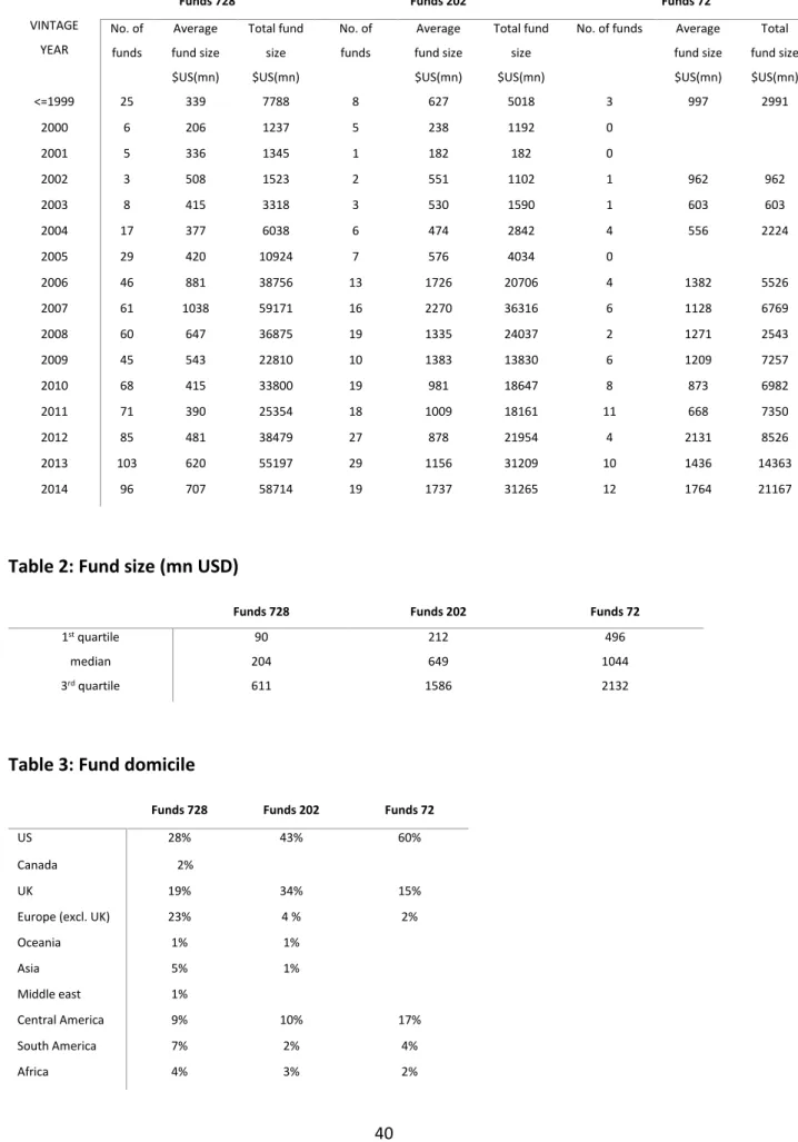
Table 1 presents the descriptive statistics for the three data samples. Details are provided by vintage year with the time period affording exploration of fund performance across different points in the global economic and financial market cycle. Looking at Funds 728, one can see the growth in fund numbers from 2004 onwards including the marked escalation in funds achieving financial close post GFC. Indeed, 81% of funds are of 2007 vintage or younger. Exploration of fund size13 highlights that the average fund size by vintage was highest for
funds with a vintage year 2007 at slightly above $1bn14. It is further noteworthy that 2009
witnessed a significant reduction of both total fund size and the number of funds launched in response to the GFC. The median fund size within the larger sample is $204mn with upper and lower quartile range at $611mn and $90mn respectively. (See Table 2). The median fund size within Funds 72 is markedly higher at $1,044mn with lower ($496mn) and upper quartiles ($2,132mn) depicting a wide range in size. The statistics infer that performance disclosure levels are greater amongst the larger infrastructure funds – perhaps a consequence of being managed by more established firms but also in line with the transparency expectations of more mainstream institutional investors who typically invest in the larger and more established funds.
<Insert Table 1> <Insert Table 2>
The number of funds declaring cash flow data has improved from 2010 onwards, nonetheless, across the vintages 2006-2014 inclusive an average of only 10% of funds that disclose IRRs also provide cash flow information. Table 3 depicts the composition of the three data sets by
13 Size is measured as the dollar amount of capital that is committed to a fund.
17
fund domicile, which indeed plays a significant part in the data performance disclosure decision with 60% of funds providing cash flow data domiciled in the US with a further 15% of funds have their location in the UK. By contrast, cash flow data for continental European and Asian domiciled funds is virtually non-existent within the Preqin dataset. The majority of funds pursue either a Core (21%) or Core Plus (34%) investment strategy (see Table 4). That means that the funds choose “safe” infrastructure projects to invest in despite their private equity structure.
<Insert Table 3> <Insert Table 4>
In terms of their geographic focus, Europe is the dominant target location for Funds 728 sample with 36% of funds (n=263) deeming this to be their primary investment location (see Table 5). The US is the second most popular destination with 189 funds. For the Funds 72 sample, US domiciled funds in this sample. Similar geographic distributions are also evident within Funds 202 with US and Europe being the primary investment markets for the fund managers. The majority of funds have employed diversified investment strategies – allowing them to assemble portfolios across the infrastructure sub-sectors. In keeping with wider global infrastructure need and depicting the wider global environmental targets renewable energy specialist funds also feature prominently. The small number of funds specialising in waste management, utilities and telecommunications is indicative of the limited opportunities available to private investors within these infrastructure sub-sectors.
<Insert Table 5>
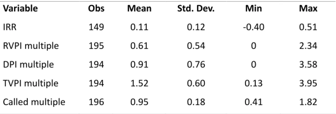
Table 6 describes performance statistics of Funds 202 on a cross sectional basis. The mean IRR of the sample funds is 11% with a sizable min-max spread of -40% and 51%, implying very diverse risk and return profiles within the funds and highlighting the heterogeneous nature of the infrastructure industry in general. Other performance indicators, such as residual to total value to paid-in capital (RVPI) and the distributed to paid-in capital (DPI) also exhibit similarly broad performance variation across the sample funds. The average RVPI is 0.61 with
18
a sample variation between 0 and 2.34 whilst the mean of DPI is 0.91 and its spread is from 0 to 3.58. An average of RVPI of 0.61 suggests that 61% of the LP’s called capital in the fund, based on the market value, remains in the fund.
The mean of DPI of Funds 202 is 0.91 and its spread is from 0 to 3.58. The DPI is also known as the realisation multiple and gives an indication of how much of the investment proceeds have been paid back to investors. In our case, on average 91% of the paid-in capital by LPs has been recovered to date. Similarly, LPs are aiming to achieve higher DPIs. The summary statistics of both metrics show that some funds outperform the majority of the funds by providing very high multiples beyond 2.
The Called multiple is the ratio of the paid-in capital divided by the committed capital by the LPs. We can see that about 95% of the capital has been drawn down by the GPs.
Finally, we look at the total value to paid-in capital (TVPI). The TVPI for Funds 202 is 1.52 with a sizable standard deviation of 0.6. The value of 1.52 means that on average the funds have surpassed the value of the paid-in capital by about 1.5-fold. However, some LPs could have made an average loss of 10%. The lowest TVPI is 0.41 suggesting a loss of 60% on the invested capital. The maximum investment multiple is 1.82 which is not as large as the other multiples. We now turn to compare the average cross-sectional performance of Funds 202 and Funds 72 in Table 7. In terms of IRR, the two samples display almost identical mean (11%) and standard deviation (12%). As regards TVPI, the larger dataset exhibits superior performance to the smaller counterpart (1.52 vs 1.28) albeit having a slightly larger standard deviation (0.6 vs 0.4). This is to be expected as funds may decide not to report bad performance and hence skew the sample to the right – the large sample. The small sample may come closer to reality with its performance metrics as it presents a more conservative picture and can serve as a lower bound on the performance spectrum.
Table 8 reports descriptive statistics for Funds 72. The sample consists of funds of varying performance ranging from a PME of 0.19 to 2.35, and IRRs from -89% to 99%. The mean vintage of the fund is 2010 and the mean fund value is $1,626 million. It can be further inferred from the table that the majority of the funds are not liquidated. They invest
19
predominately in developed economies and have greenfield assets in their portfolios.15 45%
of the funds are classified as ‘sector specialist’ funds concentrating their investments in a specific single sector, whereas 57% of them are geographically focussed funds.
<Insert Table 6> <Insert Table 7> <Insert Table 8>
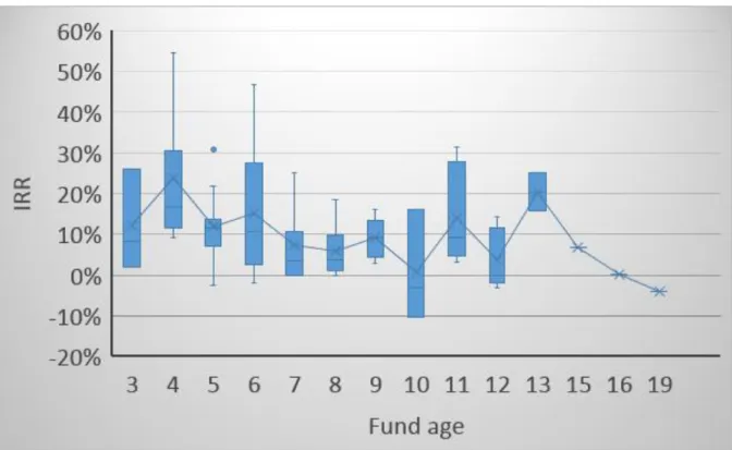
Figure 1 presents the temporal variation of average IRR relative to fund age for Funds 72. The crosses in the diagram represent the median IRRs whilst the blue boxes indicate the 25% and the 75% percentiles. The vertical lines depict the maximum and minimum IRRs for each fund age. The first two years of the fund are omitted as the cash flows of the funds are highly volatile during the inception period associated with the acquisition of the assets. IRR volatility displays irregular patterns over time with the third and fourth years exhibiting stronger variations of IRRs. For example, at year four, IRRs are in the range of about 10% to 55% with values of lower and upper quartiles of 12% and 32% respectively. The size of the spread of IRRs across funds becomes significantly smaller when the funds reach a more mature stage (at year eight). This means as funds mature, their performance converges. However, it grows again at year ten, due possibly to the funds being at a critical point of determining success and failure. The median IRR at year ten of fund’s life is close to zero and about half of the funds are showing negative returns. It must be caveated that the calculation of IRRs is highly sensitive to the patterns of cash flows of the funds, as a result the results are as good as the underlying data used in the calculations.
<Insert Figure 1>
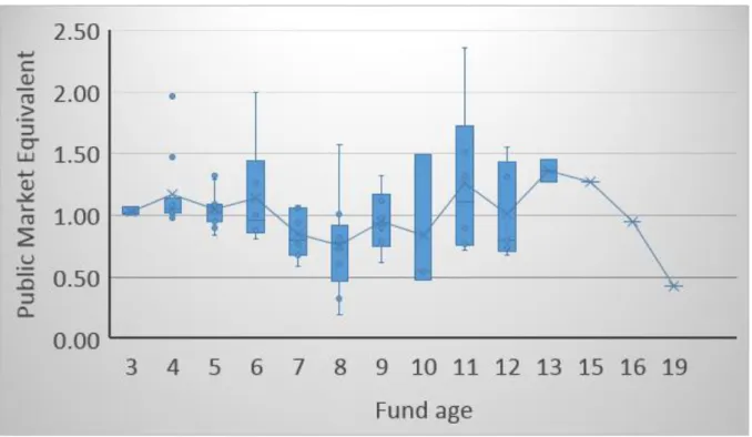
We plot the same graph using PMEs of the 72 sample funds (See Figure 2). The spreads of performance are relatively small during year 3 and year 5 with the median PME hovering around 1 – that is similar to the IRR result above. The variation of PMEs within the funds becomes consistently larger beyond year 5. Throughout year 6 to year 9, the size of the spread
15 We go through each fund manually to dissect information about the underlying assets such as whether they are greenfield or brownfield, whether they are concentrating of a specific sector or not, etc.
20
between the lower and upper quartiles of PME is in the range of 0.4 to 0.5 with the general trend of PME sloping downward. At year ten, the spread becomes larger, as is the case for IRR, suggesting better managed funds outperformed the poorly managed funds by a greater margin. This trend of spread persists through to the later stage of the funds’ life cycle (year 12) with slight improvement of PMEs being generally observed.
Lastly, we produce a graph of TVPIs against time (See Figure 3). The results are largely consistent with those of PMEs in terms of temporal variation of performance within funds and the general trends of the funds.
<Insert Figure 2> <Insert Figure 3>
Overall what is noticeable is that in the first ten years of fund’s life, IRR and PME fall gradually (this is the line). However, there is large variation in the beginning and the end of fund’s life in the performance across the funds in our sample. That may be explained by biases in the valuation – the residual value or the NAV of the funds as they draw more capital and realise investments. We can see that the variations across funds is large with some funds achieving returns of more than 15% on annual basis and others having a loss of -10%.
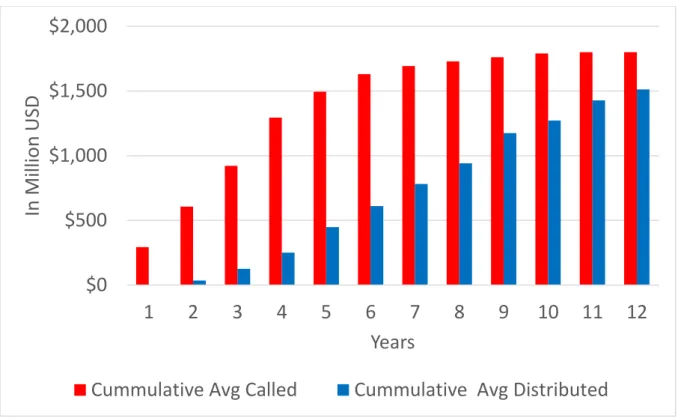
Figure 4 presents of the relationship between cumulative called and distributed capital. The amount of capital called rapidly increases during the first five years of the fund and begins to stabilise thereafter. Distribution of capital back to the LPs can begin as early as in year 2 of the fund’s life, however, the distribution grows linearly over the next ten years of the fund’s life. It requires roughly eight years for cumulative distribution to be equal to about half of the size of cumulative called capital. At the 12th year of fund’s life, still not all capital has been
distributed on average.
<Insert Figure 4>
Figure 5 depicts a comparison between average non-aggregated capital called and distributed to LPs over a fund’s lifespan. It confirms the abovementioned findings highlighting a considerable reduction of capital calls four to five years after the fund is launched and on average, distribution activities become significantly more active from year four onwards.
21
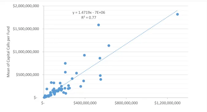
We further test the relationship between average capital calls per fund over time and the volatility of capital calls as measured by the standard deviation (Figure 6). The results are consistent with our expectations that the larger the capital calls, the greater the volatility. We perform the same analysis for distributed capital in Figure 7. Expectedly, it is observed that average distribution per fund is also positively related with its volatility. That suggests that infrastructure funds are associated with large cash flow volatilities depending on the size of the assets which have been bought and sold.
<Insert Figure 6> <Insert Figure 7>
4 Methodology
As discussed above, we conduct estimations for two sets of data – Funds 202 is a cross section of fund performance data and Fund 72 is a panel data.
The cross-sectional regression (Funds 202) is performed as:
𝑃𝑒𝑟𝑓𝑟𝑜𝑚𝑎𝑛𝑐𝑒𝑖 = 𝑐 + 𝑉𝑖 + ∑ 𝛾𝑘 𝑗
𝑗 𝑋𝑖+ 𝑒𝑖 (1)
where 𝑃𝑒𝑟𝑓𝑟𝑜𝑚𝑎𝑛𝑐𝑒𝑖, is fund i performance at the latest date available. In most cases this will be a snapshot of the current performance as of 2018. Liquidated funds will have their performance of the point of liquidation. Please note that only 21% of the funds are liquidated in the first sample. The remaining funds will be closed but still not yet liquidated as of 2018. We use a number of indicators as reported by the GPs or extracted from sources and LPs. The performance metrics include the IRR, the RVPI, the DPI and the TVPI. c is a constant; Vi stays
for fund vintage fixed effects. 𝑋𝑖 is an array of fund-level characteristics such as the log of
fund size, a dummy if the fund is invested in emerging markets, a dummy if the fund is invested only in greenfield infrastructure, a dummy if the fund is invested in regulated industries, a dummy if the fund is liquidated, and variables that capture the style of the fund and its riskiness – core, core plus, value add, opportunistic, funds-of-funds or debt fund. 𝑒𝑖 is
the error term of the regression equation. We cluster the standard errors by management firm using firm I.D. provided by Preqin in order to achieve cluster-robust covariance estimate
22
that ensures robustness within-cluster correlation. We also correct for heteroscedasticity within the regression models in line with Liang and Zeger (1986) and Wooldridge (2003).
For Funds 72 we run a panel model:
𝑃𝑒𝑟𝑓𝑟𝑜𝑚𝑎𝑛𝑐𝑒𝑖𝑡 = 𝑐 + 𝑌𝑡+ 𝑉𝑖+ 𝛽1𝑆𝑒𝑞𝑢𝑒𝑛𝑐𝑒𝑖+ 𝛽2𝑆𝑒𝑞𝑢𝑒𝑛𝑐𝑒𝑖2+ ∑ 𝛾𝑘𝑗 𝑗𝑋𝑖+ 𝑒𝑖𝑡 (2)
where 𝑃𝑒𝑟𝑓𝑟𝑜𝑚𝑎𝑛𝑐𝑒𝑖𝑡, is fund i performance at year t. Separate regressions are run for the
PME, the IRR and the TVPI. Since the data is in panel format – we control for the time variation across funds by having year fixed effects Yt. Vi captures fund vintage fixed effects. 𝑆𝑒𝑞𝑢𝑒𝑛𝑐𝑒𝑖𝑡
is the natural logarithm of the sequence number of fund i16; 𝑆𝑒𝑞𝑢𝑒𝑛𝑐𝑒
𝑖2 is the square of the
sequence and is included to capture the increasing/diminishing marginal effect of sequence.
𝑋𝑖𝑡 is an array of fund-level characteristics such as the log of fund size, the logged square of fund size, whether the fund has been liquidated, a dummy if the fund is mostly invested in developed countries, a dummy if the fund is invested in greenfield infrastructure, the share of sector concentration, the share of geographic concentration, the number of social infrastructure deals, a dummy if the fund has predominantly public sector investors, a dummy if the fund has predominantly delegated investors. Delegated investors are investors who do not invest on their own behalf – such as pension funds, etc. 𝑒𝑖𝑡 is the error term. We cluster the standard errors by management firm using firm I.D. provided by Preqin in order to achieve cluster-robust covariance estimate that ensures robustness within-cluster correlation.
We estimate two additional models to empirically test the degree of return persistence within and across subsequent private equity funds raised by the same management firm to determine the direction and level of persistence in performance.
For the persistence within the same fund, we estimate the model:
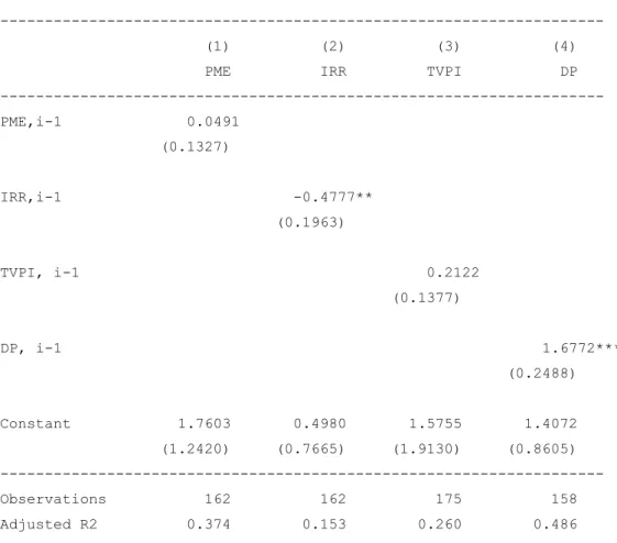
𝑃𝑒𝑟𝑓𝑟𝑜𝑚𝑎𝑛𝑐𝑒𝑖𝑡 = 𝑐 + 𝑃𝑒𝑟𝑓𝑟𝑜𝑚𝑎𝑛𝑐𝑒𝑖,𝑡−1+ 𝑌𝑡+ 𝑉𝑖 + 𝛽𝑆𝑒𝑞𝑢𝑒𝑛𝑐𝑒𝑖+ ∑ 𝛾𝑘𝑗 𝑗𝑋𝑖+ 𝑒𝑖𝑡 (3)
where 𝑃𝑒𝑟𝑓𝑟𝑜𝑚𝑎𝑛𝑐𝑒𝑖,𝑡−1 stays for the performance of fund i in the previous year, t-1.
16We employed several measures to represent the order of a fund’s sequence: (1) firm ID, (2) sister funds, (3) fund’s name and (4) sequence based on cash flow data, which will be further elucidated below.
23
For the persistence across subsequent funds of the same fund manager, we estimate the model:
𝑃𝑒𝑟𝑓𝑟𝑜𝑚𝑎𝑛𝑐𝑒𝑖𝑡 = 𝑐 + 𝑃𝑒𝑟𝑓𝑟𝑜𝑚𝑎𝑛𝑐𝑒𝑖−1+ 𝑌𝑡+ 𝑉𝑖 + 𝛽𝑆𝑒𝑞𝑢𝑒𝑛𝑐𝑒𝑖 + ∑ 𝛾𝑘𝑗 𝑗𝑋𝑖+ 𝑒𝑖𝑡 (4)
where 𝑃𝑒𝑟𝑓𝑟𝑜𝑚𝑎𝑛𝑐𝑒𝑖−1 stays for the latest performance of the previous fund i-1 of the same management company. This model will only contain the funds which have had at least one previous fund. Hence, we would have a subset of the second dataset.
5 Results
We conduct two sets of regressions – one based on reported performance metrics for the latest point in time and another based on self-calculated performance metrics premised on cash flow data. The first dataset has a cross-sectional format; the second is a panel. It is important to keep in mind that any performance measure would be problematic for illiquid funds such as infrastructure funds if it is used before the investments have been exited as there are no true market value comparables. But given that the infrastructure private market is still in its infancy, we are trying to overcome such challenges by controlling for a large number of fund-level variables. We control for industry composition, the vintage of the fund, the diversification by region or sector, etc.
5.1 Funds 202
We first run cross-sectional regressions using Equation (1) in the Methodology section. We look at four performance metrics –IRR, RVPI, DPI and TVPI. The results are presented in Tables 9 and 10. Table 9 reports the baseline results. Our main focus in Table 9 will be the risk profile of the fund. It is measured by the fund style – core, core plus, value add or opportunistic. The least risky fund will be core and core plus and the riskiest fund would follow an opportunistic style. While we would expect that risk exposure would matter for performance, our results reveal that a fund’s riskiness is not significant; at least in the cross-section, funds do not seem to show different performance based on their investment style in general. An exception is that for IRR, value-add funds have significantly higher return than core funds (core being the reference category). Furthermore, the RVPI which captures the residual value remaining in the fund is lower if the fund is opportunistic as compared to core. By way of comparison,
24
Shilling and Wurtzebach (2012) in their investigation on private equity real estate funds find that value-added and opportunistic private equity real estate investments generated higher returns than core investments, their superior returns were driven primarily by market conditions and the use of cheap debt rather than by risk exposure per se.
We control for a host of other fund-level metrics as well as fund fixed effects. Fund value does not have any impact on any of the performance indicators except RVPI. More specifically, a fund with a higher value tends to depress RVPI, seemingly suggesting larger funds are more capable of locating infrastructure investment opportunities in practice and there could be a diseconomies effect on RVPI due to the scale of investment. Another key observation emanating from Table 9 is that investing in an emerging market tends to give rise to a higher RVPI. This seems to suggest that investors are prone to be more risk-averse when investing in infrastructure assets in emerging markets. Those markets are often characterised by higher risk due to the greater degree of market immaturity, lack of transparency and uncertainty. Focusing only on greenfield assets does not necessarily imply better performance as our results indicate. Furthermore, funds investing in regulated infrastructure industries do not seem to be associated with inferior levels of performance. We would expect that funds which invest in such infrastructure projects to be regarded as less risky and hence deliver lower performance. Relative to closed funds, liquidated funds tend to have significantly lower RVPIs and higher DPIs. This is to be expected as the distributed capital should be larger at the end of fund’s life. It is evident that funds of funds tend to underperform their peers in terms of RVPI.
Overall, we use various measures of performance and find some differences in those. We see that the majority of our variables cannot explain IRRs and TVPIs in the cross-section. The adjusted R-squared for those models is 20% and 25% respectively. The highest R-squared is delivered for DPI despite the lack of significance in most variables. RVPI seems to capture well the cross-sectional variation in performance for funds that are not liquidated yet. Finally, reported investment styles are not associated with different risk premia and hence different performance in most of the cases.
25
Table 10 focuses on the effects of overshooting the target fund size and being oversubscribed. We estimate the same model as Table 9 except that now we substitute the size of the fund with the share of surplus capital. For example, if the target fund size is 100mn and the fund closed at 150mn, the fund has overshot its target by 50%. Our findings show a significantly negative relationship with IRR, RVPI and TVPI. The higher the excess capital, the worse the performance will be. That may have to do with the fund struggling to find suitable investments given how illiquid the infrastructure asset class is allied with the increased numbers of competitor funds chasing product. Even though fund managers may be experienced and well connected, the fact that they went beyond the target which already takes into account the capacity of the fund to invest and the market, means that the capital cannot be deployed as efficiently and sits unused in the form of dry powder, not generating any returns. However, anecdotal evidence suggests that fund managers would prefer to overshoot their target which may be perceived as sign of investor confidence in the fund. It may also be associated with overconfidence of GPs that they can manage the excess capital and generate returns. Not surprisingly, the distributed capital to paid-in capital (DPI) is positively linked to excess capital. The more the fund overshoots its target size, the higher the drawdowns would be and the faster capital would be distributed back to the investors.
<Insert Table 10> 5.2 Funds 72
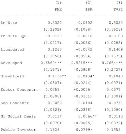
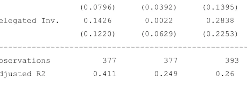
Now we turn to the panel data. Table 11 depicts the baseline results. The data is a panel of performance metrics over time for 72 funds. We follow Kaplan and Schoar (2005) and construct three performance metrics: PME, IRR and TVPI. The explanatory variables are fund characteristics such as the log of the size of the fund, the log of the square of the size of the fund, if the fund in liquidated or not, if the fund is investing in developing countries or not, if the fund is investing in greenfield infrastructure, the sector concentration of the fund in percentages, the geographic concentration of the fund, the number of social infrastructure deals in the fund, whether the fund has predominantly public sector investors and whether the fund has predominantly delegated investors. We also control for vintage fixed effects, year fixed effects and fund fixed effects.
26
It is revealed that size of fund, as well as its squared term, show no statistically significant relationship with any of the performance variables. That suggests that there are no economies of scale effects for large funds. Alternatively, we do not see any financial constraints effects for small funds, leading them to perform differently. Size in infrastructure private funds does not seem to be as key as is in general corporate finance literature. Our findings are also at odds with a number of studies on the private equity real estate funds which find a positive relationship between size and performance (e.g., Tomperi, 2010, and Fuerst and Matysiak, 2013). Moreover, many of the larger funds within the sample carry considerable levels of dry powder and whilst we control for this relative to size it is considered in the current low interest rate environment to be a dilutor of performance. Arnold et al. (2017) in their investigation into the implications of dry powder on real estate fund performance find that capital deployment speeds vary significantly across funds and over time and this variation is rarely incorporated in traditional performance metrics. The authors also highlight the significant opportunity cost investors incurred when reserving funds for uncertain capital calls. This cost of maintaining dry powder for the manager is ignored in reported performance metrics. Arnold et al. (2017) show the importance of accounting for capital deployment speeds, investment horizons, management fees, and uncalled capital as a premise for determining fund performance. Our findings ascertain that dry powder has the propensity to dilute performance and can ultimately lead to more irrational decision-making on the part of the GP – particularly for less experienced GPs in a competitive market context.
Prior research exploring the relationship between fund size and performance of private equity funds exhibit contrasting perspectives. Phalippou and Gottschalg (2009) found that fund size had a positive association with measured performance. This is consistent with the results generated by Kaplan and Schoar (2005) who identified a positive concave21 relationship
between size of fund and performance. Harris et al. (2014) found that for buyout funds, size was significant, but the inclusion of vintage year control variables diminished the level of statistical significance. The authors also found evidence of concavity for venture capital funds although the degree of statistical significance was very low. An investigation into the performance of buyout funds by Higson and Stucke (2012) identifies a weak positive relationship between size and performance. Pertinently, the authors found to be stronger for
27
funds with vintages that were less affected by economic downturns. This is significant within the confines of this investigation given the considered pro-cyclical nature of infrastructure investment whilst the impact of economic and business cycles is not universal across infrastructure sub-sectors. Overall, the finding that fund size remains insignificant across the all performance indicators highlights one aspect in which unlisted infrastructure funds differ from general private equity.
Funds investing mainly in greenfield infrastructure projects seem to be associated with significantly higher IRRs and PMEs. It is not surprising that greenfield projects are associate with higher returns as they are perceived as riskier. These findings are in contrast to those of Fisher and Hartzell (2016) who find that private equity real estate funds with high development exposures tended to underperform the wider market.
Funds investing in developed countries also perform better contrary to the expectations as one would assume that developed countries are less risky and hence would offer lower returns. It is important to keep in mind though that the majority of funds in the sample have developed country mandates. Funds targeting emerging markets generally expect to attain higher rates of return on their investment but can experience a lag effect with respect to asset maturity and value appreciation.
<Insert Table 11>
Table 11 also dissects how sector and geographic concentration of the fund impact upon its performance. To achieve this, we construct two binary measures of concentration namely sector and geographic concentration. The coefficients of both variables are statistically insignificant. Indeed, in the case of IRR sectoral concentration exhibits a negative coefficient whilst for TVPI geographic concentration yields a negative coefficient. However, both coefficients are insignificant. This may not come as a surprise given the truly global nature of the infrastructure market. These findings are distinguishable to prior research on private equity real estate funds. Aarts and Baum (2016) for example find that real estate funds with an exposure to international real estate markets dramatically underperform funds identified as “domestic”. However, the infrastructure investment market does not have the same asset
28
depth or volume of asset turnover as the real estate market while investors with a sector specific focus will invariably be required to assemble internationally diversified portfolios out of necessity.
Moreover, most funds tend to invest across various types of infrastructure, so to identify a pattern by sector concentration is not easy in first place. Funds tend to ‘keep their options open’ with respect to portfolio construction given the competitive market for asset acquisitions. The broader private equity research depicts contrasting opinions on the relative virtues of sector specialisation within funds versus a diversified mandate. Ljungqvist and Richardson (2003) test several measures of diversification and find no statistically meaningful explanatory power in respect to performance. Gompers et al. (2009) provide some evidence that focussed private equity funds deliver above average performance relative to their more diversified counterparts. This view is to some extent supported by Lopez-de-Silanes et al. (2015) who detail a weak positive relationship between performance and idiosyncratic risk.
Overall, it seems that fund performance so far is not strongly explained by fund characteristics, investment style of concentration on specific sectors. This does not seem to be due to our model fit which ranges between 25% to 64% in terms of R-squared. This in part can be attributable to the relative immaturity of the private infrastructure universe and until recently the relative absence of consistent cash flow data to permit a meaningful analysis. Unlike in the private equity sector, fund size is not seen to have a significant effect on performance and that result is robust throughout different specifications.
Now we turn to analyse performance persistence across sequence funds. The results are presented in Table 12. We estimate the same model as in Table 11 but add a variable that captures the fund sequence within the same fund management firm. For example, if the fund is the first fund of the management firm, the variable will have a value of 1. If the fund is the third follow-on fund of this fund manager, the value will be 3, and so on. We also include the square of the fund sequence to account for a non-linear relationship between performance and persistence. For example, it may be that a follow-on fund has better performance than the direct predecessor but the link may weaken going back to previous funds. Both variables