Cloud Optical Depth Retrievals from Solar Background
“Signal” of Micropulse Lidars
W.J. Wiscombe and A. Marshak Climate and Radiation Branch
National Aeronautics and Space Agency/Goddard Space Flight Center Greenbelt, Maryland
J.C. Chiu
Joint Center for Earth Systems Technology University of Maryland Baltimore County
Baltimore, Maryland E.J. Welton
Mesoscale Atmospheric Processes Branch
National Aeronautics and Space Agency/Goddard Space Flight Center Greenbelt, Maryland
S.C. Valencia
Science, Systems, and Applications, Inc., Mesoscale Atmospheric Processes Brand National Aeronautics and Space Agency/Goddard Flight Center
Greenbelt, Maryland
Introduction
Micropulse lidar (MPL) systems, developed in 1992 (Spinhirne et al. 1995), are now widely used to retrieve heights of cloud layers and vertical distributions of aerosols layers (Welton et al. 2002; Matthais et al. 2004). MPL time-dependent returned signal is proportional to the amount of light backscattered by atmospheric molecules, aerosols and clouds. However, measured photon counts must be converted to attenuated backscatter profiles, and during the process a number of noise sources need to be subtracted (Campbell et al. 2002; Welton and Campbell 2002). One source of noise is solar background light; its contribution remains significant even though the narrow field of view of MPL greatly limits the amount of solar radiation. Fortunately, this noise can be estimated from lidar returns beyond 30 km, which have no discernible backscatter.
One man’s noise is another man’s signal. The solar background noise is the solar zenith radiance, which can be used to retrieve cloud optical properties (Marshak et al, 2004; Chiu et al. 2006). We are unaware of any retrieval algorithm that uses the solar background light observed by lidars as a signal. This paper
aims to address this issue by providing a proof-of-concept for using solar background “signal” from MPL to retrieve cloud optical depth. We will also evaluate results against those retrieved from other methods, and discuss the potential of our method to shed light on aerosol-cloud interactions.
Approach
Solar background signal is estimated from lidar bins beyond 30 km in units of photon counts. For retrieval purposes, photon counts must be converted to actual radiance. This conversion is instrument-dependent. Valencia et al. (2004) demonstrated that converted solar background signal agreed with zenith radiance that was calculated from principal plane measurements of a sunphotometer at the Goddard Space Flight Center (GSFC) site of AERONET (Aerosol Robotic Network; Holben et al. 1998). In this study we followed their method and derived calibration coefficients from the sunphotometer if its data are available.
Micropulse lidars of Atmospheric Radiation Measurement (ARM) Program and of National Aeronautics and Space Administration (NASA) Micropulse Lidar Network (MPLNET) (Welton et al. 2001) both operate at a 523 nm wavelength. The general relationship between zenith radiance and cloud optical depth at this wavelength is depicted in Figure 1, based on 1D plane-parallel radiative transfer. Clearly, this relationship is not a one-to-one function. There are two cloud optical depths that give the same zenith radiance: one corresponds to thinner clouds and the other to thicker clouds. Thus, it is
impossible to unambiguously retrieve cloud optical depth from solar background signal of a one-channel MPL. To reduce this ambiguity, cloud screening is needed to distinguish thick clouds from thin clouds or no clouds. So we assume here that if a lidar beam is completely attenuated, the detected clouds correspond to the larger optical depth.
Figure 1. Downward 523-nm radiances vs. cloud optical depth calculated by the 1D radiative transfer model discrete ordinate radiative transfer (Stamnes et al. 1988) with a surface albedo of 0.05 and solar zenith angle of 60°.
Retrieval Results
Retrievals from solar background signal of MPL, presented in this section, are compared with those from: 1) one-channel radiances and fluxes at the ARM Oklahoma site; 2) two-channel radiances in the ARM MArine Stratus Radiation Aerosol and Drizzle (MASRAD) field campaign at Point Reyes, California; and 3) sunphotometer measurements at the NASA/GSFC site.
Case 1: ARM Oklahoma Site
Due to high frequency of and high climate sensitivity to thin clouds, ARM has a working group, Clouds with Low Optical Water Depth (CLOWD), to focus on microphysical properties of clouds with low liquid water paths (Turner et al. 2006). In their study, comparisons and evaluations of different remote sensing methods were performed. Among those retrieval methods, MPL was excluded because lidar measurements were supposed to work only for optical depths less than ~ 3. Beyond optical depth of 3, lidar returns are limited due to strong cloud attenuation. However, as we will demonstrate next, using solar background signal we are able to overcome this limitation and retrieve larger cloud optical depths from MPL.
One of the CLOWD cases, a single-layer overcast warm cloud at the ARM Oklahoma site on March 14, 2000, is selected for illustration. Calibrations of MPL solar background signals were conducted against 6-month observations of AERONET CIMEL. Retrievals from MPL are compared with those from one-channel zenith radiances and fluxes, which were measured by the ARM 1NFOV (one-one-channel (870 nm) narrow field-of-view zenith radiometer), and multifilter rotating shadowband radiometer (MFRSR); Min and Harrison 1996.
Figures 2a–2d present the time series, histograms, and scatter plots of cloud optical depths retrieved from MPL, 1NFOV, and MFRSR. Retrievals from these three methods show similar temporal
variations. The average cloud optical depth of MPL is 14, which is close to that retrieved from MFRSR. However, retrievals from MPL are generally 10–15% smaller than those from 1NFOV. This bias can be seen in Figure 2c as well, which reveals a good linearity below the diagonal line between retrievals of MPL and 1NFOV. Due to a smaller sample size, the linearity between MPL and MFRSR retrievals is not clear in Figure 2d.
Figure 2. Retrieved cloud optical depths for one of CLOWD case at the ARM Oklahoma site on
March 14, 2000. (a) Time series; (b) histograms; (c) a scatter plot of retrievals from MPL vs. those from 1NFOV; and (d) same as (c), but for retrievals from MPL vs. those from MFRSR. Note that MPL, 1NFOV, and MFRSR provide measurements every 30, 1, and 20 seconds, respectively.
Case 2: ARM Point Reyes Field Campaign
The MASRAD experiment was conducted at Point Reyes, California during May – September 2005. One of the scientific goals of this experiment was to understand the relationship between cloud
microphysics/structures, drizzle and radiation in marine stratus clouds (Miller et al. 2005). Due to the locations of instruments, we compared our retrievals from MPL with those from zenith radiances at 673 and 870 nm, measured by a two-channel narrow field-of-view radiometer (2NFOV). Since dual-channel radiances were observed, retrievals from 2NFOV were unambiguous (Marshak et al. 2004).
Note that sample volumes from 2NFOV and MPL are quite different. First, these two instruments have different fields of view. While 2NFOV has a FOV of 0.02 rad (1.1°), MPL has a FOV of only 100 μrad. Because of the extremely narrow FOV of MPL, the cloud situation for MPL is either clear-sky or
overcast. As a result, MPL do not suffer from the clear-sky contamination problem (Chiu et al. 2006). Second, 2NFOV has a sampling resolution of 1 second, but MPL averages over 30 seconds in order to collect a sufficient amount of photons. To make a meaningful intercomparison between retrievals of MPL and 2NFOV, only overcast cases are compared here to reduce the uncertainty resulting from two different sample volumes.
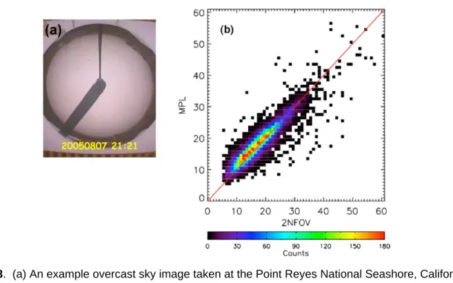
Overcast cases were objectively selected as follows: when MFRSR-retrievals were found continuously greater than 5 for at least one hour, we defined the time period as overcast. An example overcast sky image is shown in Figure 3a. Unlike the previous case, we were unable to calibrate solar background signal of the MPL against CIMEL observations in this field experiment, because no CIMEL was deployed. Therefore, we first empirically derived the calibration coefficient by comparing retrievals from uncalibrated solar background signal with those from 2NFOV for only one overcast case. This coefficient was then applied to all other 110 overcast cases.
A scatter plot of cloud optical depths retrieved from MPL vs. those from 2NFOV is shown in Figure 3b. Surprisingly, even though we only used one case to derive the calibration coefficient, for all overcast cases the majority of retrieval pairs are close to the diagonal line, and optical depths agree within 10-15%. The difference in the average cloud optical depths of the two methods is only 1.
Figure 3. (a) An example overcast sky image taken at the Point Reyes National Seashore, California during the ARM field campaign; (b) a scatter plot of retrieved cloud optical depths from MPL vs. those from 2NFOV for all overcast cases.
Case 3: Micropulse Lidar Network
Another case is based on measurements of the MPLNET at NASA/GSFC, Maryland. In contrast to previous cases, this was a broken cloud case. Because of the ambiguity of retrievals from only one channel, we manually separated thin from thick clouds. When the returned signal was not completely attenuated, it was assumed that clouds were thin.
We validated our retrievals against an AERONET CIMEL operated in “cloud mode” (Marshak et al. 2004). Figure 4a–4c show the time series of vertical backscatter profile of MPL, and corresponding retrievals from MPL and CIMEL. The mean cloud optical depths from MPL and CIMEL are 41 and 44, respectively, and their correlation is around 0.86. Except for a few outliers, errors of retrievals from MPL are around 10–15% compared to those retrieved from CIMEL.
Conclusion and Discussions
We proved that the solar background light, which is a noise to lidar applications and must be removed from lidar returns, can be used as a signal to retrieve cloud optical depth. This idea was tested for various cases, locations, and instruments. Compared to cloud optical depths retrieved from other methods, it is found that our retrievals generally agree within 10–15%. This promising result extends the retrieval ability of micropulse lidars to thicker clouds, and is no longer limited to detecting thin clouds only.
Due to the ability to retrieve vertical profiles of aerosol optical properties, lidar observations are also an essential element in the study of aerosol indirect effects (Diner et al. 2004b). To study indirect effects, it is crucial to have a dataset that includes simultaneous measurements of cloud and aerosol optical
properties at the same location. However, currently neither single ground-based instruments nor satellites can provide such datasets. Here we showed that, in principle, aerosol and cloud optical properties can be retrieved simultaneously using the same instrument. This indicates that lidar observations have great potential to serve as a unique dataset allowing us to better understand how changes of aerosol in the environment impact cloud properties.
Figure 4. (a) A time series of MPL backscatter vertical profile at GSFC on October 29, 2005. More details can be found in http://mplnet.gsfc.nasa.gov, and
http://climate.gsfc.nasa.gov/viewImage.php?id=161. (b) The time series and (c) a scatter plot of corresponding cloud optical depths retrieved from MPL and CIMEL are also shown here.
References
Campbell, JR, DL Hlavka, EJ Welton, CJ Flynn, DD Turner, JD Spinhirne, VS Scott, and IH Hwang. 2002. “Full-time, eye-safe cloud and aerosol lidar observation at Atmospheric Radiation Measurement Program sites: Instruments and data processing.” Journal of Atmospheric and Oceanic Technology 19, 431–442.
Chiu, JC, A Marshak, Y Knyazikhin, W Wiscombe, H Barker, JC Barnard, and Y Luo. 2006. “Remote sensing of cloud properties using ground-based measurements of zenith radiance.” Journal of
Geophysical Research (accepted).
Diner, DJ, RT Menzies, RA Kahn, TL Anderson, J Bosenberg, RJ Charlson, BN Holben, CA Hostetler, MA Miller, JA Ogren, GL Stephens, O Torres, BA Wielicki, PJ Rasch, LD Travis, and WD Collins. 2004b. “Using the PARAGON framework to establish an accurate, consistent, and cohesive long-term aerosol record.” Bulletin of the American Meteorological Society 85:1535–1548.
Ellsworth, WJ, KJ Voss, PK Quinn, PJ Flatau, K Markowicz, JR Campbell, JD Spinhirne, HR Gordon, and JE Johnson. 2002. “Measurements of aerosol vertical profiles and optical properties during INDOEX 1999 using micropulse lidars.” Journal of Geophysical Research 107(D19)8019.
Holben, BN, TF Eck, I Slutsker, D Tanre, JP Buis, A Setzer, E Vermote, JA Reagan, YJ Kaufman, T Nakajima, F Lavenu, I Jankowiak, and A Smirnov. 1998. “AERONET - A federated instrument network and data archive for aerosol characterization.” Remote Sensing Environment 66:1–16. Marshak, A, Y Knyazikhin, KD Evans, and WJ Wiscombe. 2004. “The ‘RED versus NIR’ plane to retrieve broken-cloud optical depth from ground-based measurements.” Journal of Atmospheric Science
61:1911-1925.
Matthais, V, V Freudenthaler, A Amodeo, L Balin, D Balis, J Bosenberg, A Chaikovsky, G Chourdakis, A Comeron, A Delaval, F DeTomasi, R Eixmann, A Hagard, L Komguen, S Kreipl, R Matthey, V Rizi, JA Rodrigues, U Wandinger, and X Wang. 2004. “Aerosol lidar intercomparison in the framework of the EARLINET project. 1. Instruments.” Applied Optics 43:961–976.
Miller, MA, A Bucholtz, B Albrecht, and P Kollias. 2005. “Marine Stratus Radiation, Aerosol, and Drizzle (MASRAD) science plan.”
Min, QL, and LC Harrison. 1996. “Cloud properties derived from surface MFRSR measurements and comparison with GOES results at the ARM SGP site.” Geophysical Research Letters 23:1641–1644. Spinhirne, JD, JAR Rall, and VS Scott. 1995. “Compact eye safe lidar systems.” Review of Laser Engineering 23:112-118.
Stamnes, K, S–C Tsay, WJ Wiscombe, and K Jayaweera. 1988. “Numerically stable algorithm for discrete-ordinate-method radiative transfer in multiple scattering and emitting layered media.” Applied Optics 27:2502–2512.
Turner, DD, AM Vogelmann, RT Austin, JC Barnard, K Cady-Pereira, JC Chiu, SA Clough, C Flynn, MM Khaiyer, J Liljegren, K Johnson, B Lin, C Long, A Marshak, SY Matrosov, SA McFarlane,
M Miller, Q Min, P Minnis, W O’Hirok, Z Wang, and W Wiscombe. 2006. “Optically thin liquid water clouds: Their importance and our challenge.” Bulletin of the American Meteorological Society (under review)
Welton, EJ, and JR Campbell. 2002. “Micropulse lidar signals: Uncertainty analysis.” Journal of Atmospheric and Oceanic Technology 19:2089–2094.
Welton, EJ, JR Campbell, JD Spinhirne, and VS Scott. 2001. “Global monitoring of clouds and aerosols using a network of micro-pulse lidar systems.” Proceedings of SPIE 4153:151–158.
Valencia, SC, CK Currie, EJ Welton, and TA Berkoff. 2004. “Development of a radiance data product using the Micropulse Lidar.” In the Twenty-second International Laser Radar Conference Proceedings, Matera, Italy, July 12-16.