February 2016 | No. 105
SYSTEMIC RISK IN DANISH BANKS:
IMPLEMENTING SRISK IN A DANISH CONTEXT
Oliver Juhler Grinderslev and
Kristian Loft Kristiansen
The Working Papers of Danmarks Nationalbank describe research and development, often still ongoing, as a contribution to the professional debate.
The viewpoints and conclusions stated are the responsibility of the individual contributors, and do not necessarily reflect the views of Danmarks Nationalbank.
As a general rule, Working Papers are not translated, but are available in the original language used by the contributor.
Danmarks Nationalbank's Working Papers are published in PDF format at
www.nationalbanken.dk. A free electronic subscription is also available at this Web site. The subscriber receives an e-mail notification whenever a new Working Paper is published. Please direct any enquiries to
Danmarks Nationalbank, Communications, Havnegade 5, DK-1093 Copenhagen K Denmark E-mail: [email protected]
Text may be copied from this publication provided that Danmarks Nationalbank is specifically stated as the source. Changes to or misrepresentation of the content are not permitted.
Nationalbankens Working Papers beskriver forsknings- og udviklingsarbejde, ofte af foreløbig karakter, med henblik på at bidrage til en faglig debat.
Synspunkter og konklusioner står for forfatternes regning og er derfor ikke nødvendigvis udtryk for Nationalbankens holdninger.
Working Papers vil som regel ikke blive oversat, men vil kun foreligge på det sprog, forfatterne har brugt.
Danmarks Nationalbanks Working Papers er tilgængelige på www.nationalbanken.dk i pdf-format. På hjemmesiden er det muligt at oprette et gratis elektronisk abonnement, der leverer en e-mail notifikation ved enhver udgivelse af et Working Paper.
Henvendelser kan rettes til: Danmarks Nationalbank, Kommunikation,
Havnegade 5, 1093 København K.
E-mail: [email protected]
Det er tilladt at kopiere fra Nationalbankens Working Papers forudsat, at Danmarks Nationalbank udtrykkeligt anføres som kilde. Det er ikke tilladt at ændre eller forvanske indholdet.
SYSTEMIC RISK IN DANISH BANKS:
IMPLEMENTING SRISK IN A DANISH CONTEXT
Contacts for this working paper:
Oliver Juhler Grinderslev
Danmarks Nationalbank
[email protected]
Kristian Loft Kristiansen
Danmarks Nationalbank
[email protected]
RESUME
Systemisk risiko i Danske banker: Implementering af SRISK i en dansk kontekst
Det markedsbaserede SRISK mål, introduceret i Brownlees og Engle (2015), benyttes til at måle omfanget af systemisk risiko i danske banker og den danske finansielle sektor som helhed for perioden 2005-15. Det systemiske risiko-bidrag for en bank måles som bankens tilbøjelighed til at være underkapitaliseret i tilfælde af en krise, dvs. når systemet som hele er underkapitaliseret. Vi finder, at SRISK var en god fremadskuende indikator for hvilke banker som behøvede statslige kapitalindskud under finanskrisen i 2007-09 og at markedsdata generelt bidrog med brugbar information i krisetider. Ifølge SRISK er den danske finansielle sektor, vurderet ved slutningen af 2015, velkapitaliseret.
ABSTRACT
Systemic risk in Danish banks: Implementing SRISK in a Danish context
The market-based SRISK measure introduced in Brownlees and Engle (2015) is used to measure the level of systemic risk in Danish banks and the Danish financial sector as a whole for the period 2005-15. The systemic risk contribution for a bank is measured as its propensity to be
undercapitalized when a crisis occurs, i.e. when the system as a whole is undercapitalized.
We find that SRISK was a very good predictor of which banks that needed public capital injections during the financial crisis of 2007-09 and that the market data generally provides useful
information in times of crisis. According to SRISK, the Danish financial sector is well-capitalized as of end-2015.
KEY WORDS
SRISK; Structural GARCH; systemic risk; market-based indicator; Danish financial sector; financial crisis.
JEL CLASSIFICATION
C32, C53, G01, G21, G32ACKNOWLEDGEMENTS
The authors wish to thank Thomas Sangill, Jacob Ejsing, Søren Lejsgaard Autrup, Anders Nysteen and colleagues at Danmarks Nationalbank for valuable comments and suggestions on preliminary versions of this paper. The authors alone are responsible for any remaining errors.
1
Introduction
We implement the systemic risk measure SRISK from Brownlees and Engle (2015) in a Danish context. SRISK combines information from market and accounting data and is used to measure the systemic risk in individual financial institutions and the financial sector as a whole.1
Our notion of the systemic risk contribution of a particular financial institution follows Acharya et al. (2012b), namely as the expected amount an institution is undercapitalized when the financial system as a whole is undercapitalized. This definition is motivated by capital shortfalls of individual financial institutions becoming systemic mainly when the system as a whole is undercapitalized, as this can give rise to fire sales and restrictions in the credit supply.
SRISK uses publicly available information from financial institutions’ balance sheets along with market data to estimate the capital shortfall institutions are expected to experience in a crisis. The use of market data separates SRISK from conventional balance sheet based stress tests. For instance, the market value of equity is used instead of the book value of equity. This ensures that the market’s forward-looking assessment of banks and their riskiness is incorporated in SRISK. Moreover, market data is available at a high frequency, ensuring that sudden shifts in systemic risk can be quickly detected. The downside is that SRISK can only be calculated for listed companies with sufficiently liquid shares.
The fact that SRISK can be computed using publicly and readily available data, makes it relatively inexpensive and quick to compute in comparison with regulatory stress tests. This has led different authors to use SRISK, along with other market-based risk measures, for computing estimates of capital shortfalls to complement and question the results from different regulatory stress tests, see among others Acharya et al. (2014), Acharya and Steffen (2014a) and Steffen (2015). The estimated total losses from SRISK and conventional stress tests are in general positively correlated (see e.g. Acharya et al. (2014) and Acharya and Steffen (2014b)).This suggests that SRISK can be used to rapidly assess the robustness under stress of financial institutions. However, the capital shortfall estimates obtained from SRISK in general differ substantially from those obtained with regulatory stress tests. One possible reason for this is the use of risk weights in regulatory stress tests. In contrast, SRISK only relies on the market’s assessment of risks in banks, illustrating how SRISK can be considered a market-based stress test.
This paper calculates SRISK for the four major listed banking groups operating in Denmark: Danske Bank, Jyske Bank, Sydbank and Nordea. We find that SRISK indicates a shortage of capital under stress during 2008 for all banks. The decrease in capitalization began in early 2007 and Danske Bank faced a capital shortage as early as February 2008 according to SRISK. The information from market data were a substantial driver behind the decrease in capitalization and the capital shortfall, underlining how SRISK is a market-based stress test. SRISK for the Danish financial sector reached its maximum in March 2009. This was just after Bank Rescue Package II (the ”credit package”) was adopted in Denmark. Among other things, the credit package allowed credit institutions that were deemed solvent to voluntarily apply for government-funded hybrid capital. We find that SRISK in most cases was able to predict the subsequent capital injections quite well and that SRISK provides early warning indications over and above what conventional risk-drivers provide.
Finally, the extension of SRISK, ”Structural GARCH” (SGARCH), presented in Engle et al. (2014) has been incorporated into the modelling framework. This extension enables us to explicitly model the changes in equity volatility occurring due to changes in a firm’s capital structure. SRISK calculated using the Structural GARCH model appears to provide earlier signals regarding changes in capitalization, although the differences relative to the normal SRISK are quite small.
1The Volatility Lab at New York University is already calculating SRISK for many international financial
2
Model
The purpose of SRISK is to measure the capital shortfall a financial institution is expected to experience in case of a crisis, cf. Brownlees and Engle (2015). SRISK attemps to model themarket value of a financial firm’s assets in the case of a future crisis using information from both equity markets and balance sheets. A crisis is approximated with a general stock market crash. Hence, SRISK can be regarded as a market-based alternative to the conventional regulatory stress tests.
2.1
Calculating SRISK
SRISK for firmiat timetis defined by
SRISKi,t=EtCSi,t+h|Crisist:t+h,
whereCS is short for ”Capital Shortfall” andt+his the future point in time at which the crisis occurs.
That is, SRISK measures the vulnerability of financial firms in the presence of a systemwide shock. There are other market-based measures in the literature that instead seeks to capture risk spill-overs from a particular firm to the system, one of the most popular being ∆CoV aRintroduced in Adrian and Brunnermeier (2011). As emphasized by Acharya et al. (2012a), the choice of model is essentially a question of causality,”Are firms weak because of the crisis, or does the crisis happen because the firms are weak?”, Acharya et al. (2012a) p. 62. They argue that a systemic crisis and weak firms are jointly endogenous variables with no implication of causality. They further argue, that given the probability that some common shock is affecting both the firm and the market, it makes more sense to look at tests for weaknesses of individual firms as a function of market weakness. SRISK does exactly this.
To calculate SRISK, one needs to specify three things: 1. How to measure the capital shortfall.
2. How a crisis is defined.
3. How to relate the crisis and the capital shortfall, such that the capital shortfall conditional on a systemic event can be estimated.
Each of these three questions will be dealt with in separate sections below. 2.1.1 Measuring the capital shortfall
Following Brownless and Engle (2015), the capital shortfall for firmiat timet is defined by
CSi,t=k·Ai,t−M Vi,t (1)
=k·(Di,t+M Vi,t)−M Vi,t, (2)
whereM Vi,t is the market value of equity,Di,tis the book value of debt andAi,t =Di,t+M Vi,t is
what Brownlees and Engle (2015) denote as the ”quasi assets” for firmiat time t. The quasi assets can be interpreted as the equity market’s assessment of the firm’s assets, as the market value of the outstanding shares is used instead of the book value of equity. Finally,k is the prudential capital fraction, i.e. the minimal share of the quasi assets firm i is meant to fund using equity. Given that the current proposal from the Basel Committee of Banking Supervision is a leverage ratio of 3 pct., k = 3 pct. has been used when implementing SRISK in Danmarks Nationalbank and
will also be used for the remainder of this paper.2 With the current regulatory framework, capital
requirements are based on risk weighted assets. Furthermore, the capital requirements are (to some extent) allowed to be met with other types of capital than equity, e.g. hybrid and subordinated debt. With SRISK, only the market value of equity is taken into account and the assets are not risk weighted per se. Instead, the market’s view on the riskiness of the assets is incorporated. The market’s view on riskiniess is taken into account in two ways, 1) the more risky a financial institution is, the harder future cash-flows will be discounted. All else equal this will lead to a lower market value and lower capitalization. 2) The more risky a financial institution is, the more the market value will decrease in case of a crisis. This will lead to a lower capitalization in case of a crisis. In section 4.4 an implicit market-based risk weight capturing the risk from effect 2) will be calculated using SRISK. The fact that the market’s view on riskiness is incorporated, also implies that the capital requirement of 3 pct. of quasi asset cannot be interpreted as a leverage ratio. This is because the capital requirement has to be met in case of a crisis, implying that more capital than 3 pct. of quasi assets is needed during normal times in order not to be undercapitalized according to SRISK. How much more, depends on the degree of riskiness of the financial institution.
2.1.2 Definition of a crisis
The crisis in SRISK is defined to be a general stock market crash over the nexthdays of at least
C percent
Crisist:t+h={RM,t:t+h≤C}, (3)
withRM,t:t+h being the cumulative market return over the nexthdays.
However, after determining that this constitutes a crisis, one still needs to decide a. Which stock market to consider?
b. How much should the market fall before the fall constitutes a crisis? c. What is a reasonable time horizon for the market crash to occur over?
The choice of market depends on what stock market the model-developer believes is best at capturing the risks faced by the financial firms of interest. The focus of Danmarks Nationalbank is Danish financial firms, which seemingly makes a Danish index the obvious choice. However, as the leading Danish index (OMX C20 Cap) is dominated by a few firms, the evolution in this index might not be representative of the risks faced by financial firms.3 Another reason this index might
not be ideal to use, is that the biggest Danish financial institution, Danske Bank, also has quite a large weight in OMX C20 Cap. This implies that some degree of covariation between the market and Danske Bank will exist per construction.
Alternatively, given that Denmark is a small open economy, many of the relevant risks would be captured using a broad European index (e.g. STOXX Europe 600). Using an index this broad, would also fit well with the rather diverse Danish financial sector (besides the actual bank, the Danske Bank group for instance includes an insurance subsidiary, a mortgage bank as well as foreign branches), since the chosen index ultimately should be broad enough to capture the risks that are judged to be relevant for the Danish financial sector as a whole. Therefore STOXX Europe 600 is our preferred index for calculating SRISK going forward.
2Brownlees and Engle (2015) use the somewhat stricterk= 5.5 pct. for European financial institutions and k= 8 pct. for US financial institutions.
3In fact, OMX C20 Cap was introduced in 2011 as a response to the very large weight obtained by a few firms
in OMX C20, particularly the medical firm Novo Nordisk. However, the maximum weight in OMX C20 Cap is 20 pct. which still implies that e.g. Novo Nordisk is allowed to account for a large fraction of the index.
If one were to focus on a specific source of risk, a potentially relevant index to use as the market could be the one for European banks (EURO STOXX Banks). The interpretation of SRISK would then be the expected capital shortfall of Danish banks conditional on an European banking crisis. A relevant channel of risk in this case could be the linkages between Danish banks and dominant European banks. However, when focusing on sub-markets, a narrower set of risks are implicitly incorporated into the model relative to when using a broad market index. Hence, in SRISK, where the shock can only come from one factor, it might be too restrictive to focus on sub-markets. One way to address this issue could be to do as Engle et al. (2015), who introduce a multifactor model to explain the return-dynamics of financial firms. In such a setting, it could be interesting to introduce sub-markets, such as the one for European banks. In turn, this would make it possible to disentangle specific shocks (such as those to European banks) from more common shocks (e.g. to Danish growth prospects).
Regarding the size of the market crash (C) and the time horizon over which it occurs (h), Engle et al. (2015) use C = −40 pct. and h = 132 trading days (6 months). As illustrated in Figure 2.1, this corresponds quite well to what was observed during the financial crisis for some relevant indices. Therefore, in order to mimic the stress experienced during the financial crisis,C =−40 pct. and h = 132 days have been used when implementing SRISK in this paper. It should be noted, that the market return is evaluated at the end of the six months. This implies that the market could have decreased by 40 pct. before the six months and then rebounded, without this being designated as a crisis.
Figure 2.1: 6M change in stock indices and Danish GDP, 2000-2015.
The 6M change in nominal Danish GDP is also included in Figure 2.1. There appears to be some degree of comovement between stock prices and GDP, with stock prices tending to lead GDP. This indicates that the stress in SRISK is related to the macroeconomic stress used in many conventional balance sheet based stress tests.
2.1.3 Calculating the conditional capital shortfall
Using the earlier definition of SRISK along with the definitions of capital shortfall and a crisis, the following expression for SRISK can be written
SRISKi,t =Et[CSi,t+h|Crisist:t+h] (4)
=Et 3%· Di,t+132+M Vi,t+132 −M Vi,t+132 RM,t:t+132≤ −40% . (5)
That is, SRISK measures the capital shortfall relative to a capital requirement of 3 pct. of total assets in 6 months given that the stock market has decreased by 40 pct. What remains is to map the hypothetical stock market crash into the value of assets. I.e. to model how a hypothetical stock market crash would affect the value of debt and the market value of the firm. Brownlees and Engle (2015) make the simplifying assumption that the expected value of the debt will be unaffected by the crisis, i.e. that
Et[Di,t+132|RM,t:t+132≤ −40%] =Di,t. (6)
In practice, this assumption might not hold due to e.g. resolution regimes with bail-in or the use of hybrid debt. Both of these features could imply that the nominal value of debt will be downscaled when a financial institution is in trouble, leading to a decrease in the capital shortfall. Despite these drawbacks, the assumption in equation (6) makes the model a lot easier to work with. It has therefore also been adopted when implementing the model at Danmarks Nationalbank. Therefore a potential capital shortfall calcualted using SRISK will tend to constitute an upper bound.
What remains, is to obtain an estimate of the expectation of the market value of the firm conditional on a general stock market crash. This can be split into two parts, one stating what the market value is today and a second containing the expectation of how many percent the market value will decrease conditional on a general stock market crash. Brownlees and Engle (2015) denote the latter the ”Long Run Marginal Expected Shortfall” (LRMES). I.e.
Et[M Vi,t+132|RM,t:t+132≤ −40%] =M Vi,t·(1 +LRM ESi,t),
withLRM ESi,t=E[Ri,t:t+132|RM,t:t+132≤ −40%].
Given that the market value can be observed in the market, what remains is an estimate of LRMES. To obtain this, an econometric model is needed. As financial markets are known to exhibit changing dynamics, it is essential to use dynamic models that are able to capture chang-ing interdependencies and volatilities. The use of dynamic models is particularly important in this context, as the aim essentially is to measure the current degree of dependence between the stock market and a particular financial institution. Brownlees and Engle (2015) suggest using the ”Dynamic Conditional Correlation” (DCC) model to model the time-varying dependence between the stock market and a particular financial institution. To model the time-varying variances for the univariate return series, they suggest using GARCH-models. The joint model is denoted the ”GARCH-DCC model”. To underline why the usage of dynamic models is a must when calculating SRISK, Brownlees and Engle (2015) compare SRISK results obtained when using different models for estimating LRMES. They find that SRISK-estimates obtained using the dynamic GARCH-DCC model Granger-causes SRISK-estimates using both static and other dynamic models. This lead them to conclude, that the GARCH-DCC model is the most appropriate model for modelling LRMES and SRISK, as it delivers the most timely signal.
Going forward, joint returns are assumed to be jointly normally distributed conditional on information until time t−1. Importantly, both correlations and variances are allowed to vary over time. This implies that changes in the dependence structure between the stock market and a particular financial institution are captured by the general model stated in equation (7).
ri,t rM,t Ft−1∼ N µi µM , σ2
i,t ρi,tσi,tσM,t ρi,tσi,tσM,t σ2M,t
, (7)
withri,t being the daily return at timet,µi being the unconditional mean (it is assumed that the
conditional and unconditional mean is the same) andσi,t2 andρi,tbeing the conditional variance and
correlation respectively. As mentioned, the variances are modelled using univariate GARCH-models and the correlations using a multivariate DCC-model.
2.1.4 Modelling the conditional variance
For modelling the conditional variances, an asymmetricGJ R(1,1) model of Glosten et al. (1993) with Gaussian standardized residuals is chosen. That is, the conditional univariate returns are assumed to follow the process below. Note that the return-series are demeaned by subtracting the average. The demeaned series are denoted ˜r.
rj,t=µj+ ˜rj,t ˜ rj,t=σk,t·j,t, j,t∼ N(0,1) σj,t2 =ωj+ αj+γj·1˜rj,t−1<0 ·˜r2j,t−1+βj·σ2j,t−1, forj =i, M.
The above model captures stylized facts for equity returns such as volatility clustering, fat tails and negative skewness.
2.1.5 Modelling the conditional correlation
To allow for features such as time-varying correlations and ”correlation-clustering”, a DCC-model (see Engle (2009) for a thorough introduction to the DCC-model) is used for modelling the condi-tional correlations. With the DCC-model, the so-called ”pseudo-correlations”,Qi,t, are modelled
by Qi,t= (1−αic−βic)Si+αic i,t−1 M,t−1 i,t−1 M,t−1 0 +βicQi,t−1.
To ensure that an actual correlation matrix is obtained (i.e. one with 1’s on the diagonal and the correlations as the off-diagonal elements),Qit is normalized as below.
Corr i,t−1 M,t−1 =Ri,t = 1 ρi,t ρi,t 1
=diag(Qi,t)−1/2Qitdiag(Qi,t)−1/2,
withRitbeing the dynamic correlation matrix capturing the linear dependence between firmiand
the stock market anddiag(Qi,t) being a diagonal matrix only containing the diagonal elements of Qi,t. The parameters are restricted to ensure that the conditional correlation matrix is positive
definite.
2.1.6 Estimation
Combining the assumption of conditional joint Normality of the returns with the GARCH- and DCC-equations above, the log-likelihood of the demeaned data set,{˜r1, ...,˜rT}, can be written as
L=−1 2 T X t=2 (2·log (2π) + log|Ht|+ ˜r0tH− 1 t r˜t),
withHtbeing the dynamic covariance matrix in equation (7).
The parameters can be estimated using two approaches. The first is the time-consuming one-step approach, in which the full likelihood is maximized. Alternatively, the likelihood can be maximized in two steps, by first estimating the parameters in the univariate GARCH-models, and then using the estimated standardized residuals for estimating the parameters in the DCC-model. Engle (2009) explains how the two-step approach is consistent and in most cases will be very close to the one-step approach. As the two-step approach is less time-consuming than the one-step approach, we use the two-step approach in this paper.
2.1.7 Estimating LRMES
Using the GARCH-DCC model introduced above, one can obtain a model for tomorrow’s joint firm and market returns conditional on past information. That is, the best current estimate for the dependence structure between the market and the firm given the available information. What remains, is to use this model for estimating the LRMES. I.e. estimating how much a given financial institution will lose in market value conditional on a general stock market crash of 40 pct. in 6 months.
LRM ESi,t =Et[Ri,t:t+132|RM,t:t+132≤ −40%].
Brownlees and Engle (2015) suggest using a stepwise simulation based procedure, in which the estimated GARCH-DCC model is used to obtain the LRMES predictions.
Before going through the steps, it is worth noting that the standardized innovation for firm i
conditional on the market innovation is given by
εi,t= r i,t−µi σi,t −ρit rM,t σM,t / q 1−ρ2i,t. (8)
This is a consequence of the joint return series being assumed to follow a conditional Gaussian distribution (see equation (7)). Equation (8) is used several times during the stepwise procedure, which is explained below.
1. Construct the GARCH-DCC standardized innovations. Note that we are using log-returns throughout this paper.
M,t= rM,t−µM σM,t andεi,t= r i,t−µi σi,t −ρit rM,t−µM σM,t /q1−ρ2 i,t, (9) fort= 1, ..., T.
2. Sample with replacement S×hpairs of standardized innovations, [M,t, εi,t]. This provides
one with S pseudo-samples of lengthh(i.e. 6 months) of the GARCH-DCC innovations. 3. Plug the pseudo-sample of the market innovations, [s
M,T+l]l=1,...,hfor each of thes= 1, ..., S
samples recursively into the GJ R(1,1) model estimated for the market earlier, while using
σ2
M,T as initial value. This yieldsS simulated paths of returns for the market.
4. Use the parameters from the DCC-model to calculateρs
i,T+1for each of theSpseudo-samples
where the market decreased by at least 40 pct. after 6 months 5. Calculate the standardized residual for firmiusing
si,T+1=εsi,T+1q1−(ρs i,T+1)2+ρ s i,T+1 s M,T+1. (10)
6. Use the demeaned return and standardized residual from periodT as inputs in theGJ R(1, 1)-model estimated for firmito calculate the conditional variance for firmi, (σi,Ts +1)2.
7. The periodT + 1 return for firmican now be calculated as
ri,Ts +1=q(σs i,T+1)2
s
8. Undertake step 4-7 recursively for T +l, with l = 2, ..., h to obtain daily returns for the samples where the market has decreased by at least 40 pct.
rsi,T+l
l=1,...,h
FT, s= 1, ..., S.
9. Calculate the arithmetic return for each simulated path as
Rsi,T:T+h= exp h X l=1 rsi,T+l −1.
10. Finally, calculate LRMES as the average return for firm i given the market has decreased by at least 40 pct. To ensure that some extreme observations do not affect the LRMES too much, LRMES is calculated when disregarding the 1 pct. lowest and highest returns for firm
i. LRM ESi,T = PS s=1Ri,T:T+132·1RM,T:T+132<−40% PS s=11RM,T:T+132<−40% .
Figure 2.2 illustrates the 6 month return for 50,000 simulations for the STOXX Europe 600 and Danske Bank. The data is simulated by estimating a GARCH-DCC model and then following the simulation procedure described above. Besides illustrating how relatively few simulations generate market returns below -40 pct. (illustrating how many simulations are needed to compute LRMES) the chart also illustrates several other points. First, the positive correlation between STOXX Europe 600 and Danske Bank (see Table 3.1 in Section 3) implies that the simulated returns are also positively correlated. Second, the higher volatility of the Danske Bank share leads to a wider distribution of Danske Bank returns than that of the market returns. Essentially, LRMES is the average of the observations stated in the chart on the left hand side, which are mostly negative due to the positive correlation between STOXX Europe 600 and Danske Bank.
Essentially, SRISK combines the equity market’s assessment today of a given financial institution (through using the market capitalization of an institution instead of the book value of equity) with the information obtained from LRMES to evaluate the capitalization of a financial institution in case of a crisis. Having an idea of what risks LRMES capture are therefore essential to understand the risks SRISK capture. As illustrated below, LRMES is a function of both an institution’s β
(it’s systematic risk), the equity market’s expected shortfall as well as the instition’s joint tail risk with the market, i.e. its tendency to crash if the market crashes. The use of dynamic econometric models allow both effects to vary over time.
To illustrate this more formally, Benoit et al. (2013) evaluate LRMES for a one-period market decrease of c pct. (which they denote the ”Marginal Expected Shortfall”, MES) and find the following closed form expression (this can also be derived using equations, (9), (10) and (11))
M ESi,t =Et−1 ri,t rM,t< c σM,t =σi,t·ρi,t·Et−1 M,t M,t< c σM,t +σi,t· q 1−ρ2 i,t·Et−1 εi,t M,t< c σM,t = σi,t σM,t ·ρi,t·Et−1[σM,t·M,t|σM,t·M,t< c] +σi,t· q 1−ρ2 i,t·Et−1 εi,t M,t< c σM,t =βi,t·Et−1[rM,t|rM,t< c] +σi,t· q 1−ρ2 i,t·Et−1 εi,t M,t< c σM,t .
Figure 2.2: Simulated 6M cumulative returns for STOXX Europe 600 and Danske Bank.
Note: The returns have been simulated using 50,000 simulations and data from 1999-2015.
Source:Bloomberg and own calculations.
Under the assumption of joint normality (see equation (7)) the last term will be zero. That is, under the distributional assumption in equation (7)4, M ES is essentially a function of the systematic
risk of a firm; βi,t, and the expected shortfall of the market; Et−1[rM,t | rM,t < c]. However,
if there is tail dependence in the data not captured by the distribution in equation (7), then
Et−1[εi,t|M,t< σc
M,t] will enter with a non-zero value. Given that SRISK (and LRMES) intends
to measure systemic, and not systematic, risk it would be a bit unfortunate ifEt−1[εi,t |M,t<σc
M,t]
was indeed zero.
However, since the empirical distribution of [M,t, εi,t]t=1,...,T is used, the distribution in
equa-tion (7) is not imposed on the data, implying that (LR)MES is not necessarily described entirely by the systematic risk of the firm and the expected shortfall of the market.5 To investigate whether
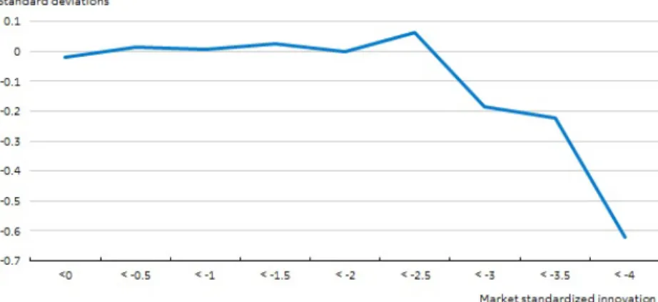
there is any lower tail dependence betweenM,tandεi,t, Figure 2.3 plots the mean ofεDanske Bank,t
conditional onM,tbeing below certain thresholds. If the assumption of joint normality is correct,
we would observe E[εi | M < c] = E[εi] = 0 due to independence. In contrast, the chart
il-lustrates how there appears to be some lower tail dependence in the empirical distribution for [M,t, εi,t]t=1,...,T. Cf. that the conditional average ofεi,tis substantially lower than its average of
0 when the market innovation is−3 standard deviations or lower. Although the market innovation is only this low for a minor part of the sample (0.5 pct. for the present dataset), it is these inno-vations that are relevant when simulating the paths in which the market decreases by at least 40 pct. In sum, this suggests that the assumption of Et−1[εi,t |M,t < σM,tc ] = 0 is not correct and
that the (LR)MES of a given firm is not solely determined by the firm’s systematic risk and the
4Or other elliptical distributions in which the dependence between two return series is captured entirely by their
correlation.
5When assuming that the joint returns are normally distributed, one implicitly assumes thatε
i,tandM,tare
independent, since the correlation between the standardized residuals fully captures the entire dependence structure. However, when using the empirical distribution one allows for tail dependence, implying thatEt−1[εi,t|M,t<σM,tc ]
market’s expected shortfall due to tail dependence in the data. It also illustrates how the model is relatively flexible, and is able to capture features such as time-varying tail dependence in the data.
Figure 2.3: Expectation of standardized Danske Bank innovation conditional on market standard-ized innovation.
Note:Data from 1 January 1999 to 26 November 2015 have been used. The market is STOXX Europe 600.
Source:Bloomberg and own calculations.
2.1.8 Summing up: Comparing SRISK with balance sheet based stress tests
In conclusion, SRISK is quick and relatively inexpensive to update due to the usage of publicly available information and the computationally efficient models and simulation procedures described earlier. This is in contrast to regulatory stress tests, where data gathering can be cumbersome for both banks and regulators.
Furthermore, the use of market data implies that all publicly available information as well as the market’s expectations towards future events are incorporated in SRISK. Also, SRISK only depends on the market’s assessment of the riskiness of the banks, the Basel risk weights are not incorporated. One of the arguments for this, is that the risk weights of IRB-banks (”Basel risk weights”) could be subject to model risk or even outright manipulation (Grill et al. (2015)). These potential flaws of conventional risk-weighted capital ratios are not present in SRISK. Besides aggregating information, market data also has the advantage of being available with a high frequency, ensuring that SRISK can be updated more frequently than regulatory stress tests. Finally, using a broadly based market decline as the stressscenario implies that a lot of factors can give rise to stress in banks. As a consequence, it becomes more difficult for banks to ”adjust” to the outcome in SRISK, such that they look more robust than they are in reality. Something which they might be able to with regulatory stress tests where the scenarios are easier to predict and adjust to (Glasserman et al. (2015)).
Although there are several advantages related to using SRISK, some words of caution are in place as well. For instance, given the reliance on market data, SRISK cannot be calculated for non-listed institutions nor does it provide meaningful results for banks with illiquid shares, as the dependence with the market would be difficult to measure. In relation to this, model risk should also be mentioned. I.e. the uncertainty related to what actually constitutes the data generating process. Dan´ıelsson et al. (2015) criticize the marginal expected shortfall (MES) measure for being prone to model risk, by illustrating how MES-estimates differ substantilly depending on what econometric model is used, particularly around times of crisis where they are most important. Model risk will
always be present. However, the relatively flexible and dynamic model and simulation procedure used by Brownlees and Engle (2015) and reused in this paper, should reduce problems related to model risk.6
Another point worth mentioning, is that the aggregating nature of market data makes it diffi-cult to pinpoint specific weaknesses for banks that, according to SRISK, are short of capital. In our view, this implies that SRISK (and other market-based measures) can only complement (not replace) conventional balance sheet based stress tests, as the latter can be used to pinpoint specific weaknesses of banks and their business models. In relation to this, it is also worth mentioning that the aggregating property of market data implies that potential new sources of weaknesses (e.g. cyber risk) might be captured by a firm’s market value, while it might not be captured when using conventional risk models. In our view, this is a major advantage of the aggregating property of market data. However, regulatory stress tests can also reveal information unknown to the markets. Different studies (see e.g. Morgan et al. (2014) for the US and Petrella and Resti (2013) for Europe) find that stress test results affect stock prices for the banks and serve a role in mitigating issues related to bank opacity. This again illustrates how market-based measures can only complement regulatory stress tests.
Finally, market data tend to exhibit some degree of procyclicality, e.g. due to changing risk premias without these changes necessarily being driven by fundamentals. Hence, there is the risk that banks could appear too well-capitalized in good times and vice versa. However, this is also a risk with e.g. balance sheet based stress tests and when using Basel risk weights, as these could attach too much weight to recent events. Instead, one advantage of using high-frequent market data is, as mentioned, that new information is incorporated quickly such that ”misperceptions” by the market can be corrected in a short period of time. Importantly, both market-based and regulatory stress tests do not say anything about the likelihood of a crisis - only the capitalization given a crisis.
A point raised by Brownlees and Engle (2015) is that off-balance exposures are not explicitly included in SRISK. However, if the off-balance exposures are of a certain size and the market at-taches some probability to the associated risks materializing, the stock price of the firm and the comovement with the market should be impacted. Hence, we would expect that off-balance expo-sures are in most cases indirectly incorporated where they matter.
The abovementioned points suggest that SRISK is a nice complement to regulatory stress tests, providing regulators with a quickly available and up-to-date market-based estimate of the capi-talization under stress of listed banks. In accordance with this, Acharya and Steffen (2014a) use SRISK (among other stressed and unstressed capital shortfall measures) to provide initial esti-mates of which banks that most likely would need capital under the subsequent ”Comprehensive Assessment” performed by the ECB and published in October 2014.7 After the results were pub-lished, Steffen (2015) used different market-based measures (including SRISK) to evaluate whether subsequent measures undertaken by banks exhibiting capital shortfalls under the comprehensive assessment appeared to have had any effect according to the financial markets.
As explained in-depth in Section 4.4, there are relatively large discrepencies between the risik-iness of a bank when measured using the Basel risk weigths or using the market’s assessment. In turn, this implies that capitalization under stress measured using SRISK and regulatory stress tests tend to differ somewhat. However, SRISK provides estimates of the loss conditional on a crisis, which appears to be somewhat similar to the total losses obtained in regulatory stress tests.
6As mentioned earlier, Brownlees and Engle (2015) found that the GARCH-DCC model tended to produce
SRISK estimates that Granger-caused estimates obtained using alternative models. This suggests that the DCC model is a good model to use when calculating SRISK.
3
Data
The empirical analysis focus on the three Danish banking groups: Danske Bank A/S, Sydbank A/S and Jyske Bank A/S along with the Nordic banking group, Nordea Bank AB. All three Danish institutions and the Danish subsidiary of Nordea Bank AB have been designated SIFIs by the Danish authorities. They were behind approximately 60 pct. of total lending and Danske Bank, Sydbank and Jyske Bank alone had assets worth more than 200 pct. of Danish GDP per 30 June 2015. Since SRISK requires stock prices and market values as inputs, it is only possible to consider the banks at group level. However, since transfers within a group are possible if parts of it are failing, it may be the most appropriate to look at vulnerabilities at the group level. Going forward, the terms ”banks” and ”banking groups” will be used interchangeably.
To compute SRISK, three things are required. 1) Market capitalization for the financial insti-tutions of interest, 2) stock prices for the banks and the stock market index of interest8 and 3) the book value of debt9. The market capitalization and stock prices are extracted from Bloomberg. As much data as is available has been extracted for each bank. All series are daily closing values in Euros which subsequently have been converted into DKK using exchange rate data from Danmarks Nationalbank. The time series for total debt mainly stems from SNL financial. However, gaps in time series have been filled out with data from Bloomberg, when available. When computing LRMES, return-data from 3 January 1999 to 26 November 2015 has been used. SRISK has been computed on a monthly basis for the period January 2005 - November 2015.
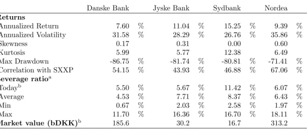
Table 3.1: Summary Statistics
Danske Bank Jyske Bank Sydbank Nordea
Returns Annualized Return 7.60 % 11.04 % 15.25 % 9.39 % Annualized Volatility 31.58 % 28.29 % 26.76 % 35.86 % Skewness 0.17 0.31 0.00 0.60 Kurtosis 5.99 5.77 12.38 6.49 Max Drawdown -86.75 % -81.74 % -80.81 % -71.41 % Correlation with SXXP 54.15 % 43.93 % 46.88 % 67.06 % Leverage ratioa Todayb 5.50 % 5.67 % 11.42 % 6.07 % Average 4.53 % 7.71 % 8.37 % 6.43 % Min 0.67 % 2.03 % 2.58 % 1.97 % Max 11.70 % 16.36 % 16.70 % 18.11 % Market value (bDKK)b 185.6 30.2 16.7 313.2
aDefined as market value of equity divided with the value of the quasi assets. bFor 26 November 2015.
Summary statistics for the return-series as well as for leverage and market capitalization are stated in Table 3.1. As illustrated, the return-series all have fat tails and are skewed (with the exception of Sydbank). Also, they have exhibited an average correlation of around 50 pct. with the STOXX Europe 600 for the period 1999 - 2015. The figures for the market-based leverage as of today, are around 6 pct. for Danske Bank, Jyske Bank and Nordea while it is above 11 pct. for Sydbank. The marked-based leverage was below 3 pct. for all banks during the financial crisis, implying that the capital requirement in SRISK would have been violated even with a LRMES of
8To ensure that dividend payments are taken into account, total return series are used instead of raw stock
returns.
0. In terms of market capitalization, Nordea and Danske Bank are by far the biggest banks in the sample, with market values of equity of around 313 and 185 billion DKK per 26 November 2015, respectively.
4
Results
4.1
Calculating SRISK for individual financial institutions
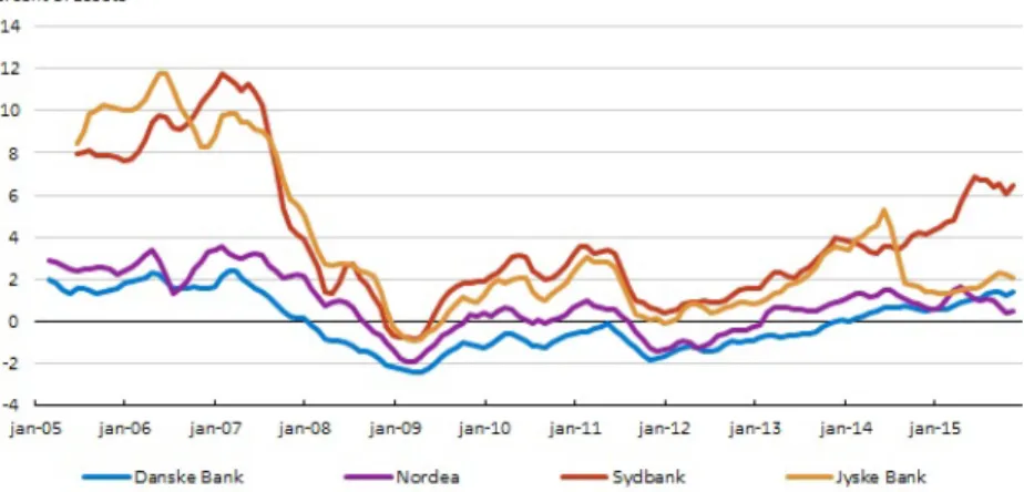
To evaluate the historical capital adequacy of banks relevant for the Danish financial sector, the capital surplus relative to quasi assets10is pictured in Figure 4.1 for the four banks; Danske Bank, Sydbank, Jyske Bank and Nordea.11
The figure illustrates how, according to SRISK, all four banking groups experienced a capital shortfall under stress relative to the capital requirement of 3 pct. of quasi assets, during the financial crisis. Danske Bank experienced a capital shortage as early as February 2008. Common for all four banking groups was that their capital surplus, according to SRISK, started to decline in the late spring of 2007.
According to SRISK, the capital needed in case of a new severe shock reached a maximum in March 2009 for all four institutions under consideration. The aggregate capital shortfall under stress corresponded to around 160 billion Danish kr. (8.8 pct. of GDP in 2008). During the European sovereign debt crisis several of the banks also exhibited capital shortages according to SRISK. In the latter years, SRISK indicates that the capitalization of the banks has improved substantially.
Some additional points regarding the development in SRISK are worth mentioning. First, the sharp decrease in capital surplus relative to the quasi assets for Jyske Bank during 2014 stands out. This is due to the merger between Jyske Bank and the danish mortgage bank BRFkredit on the 30th of April 2014. This led to a substantial increase in both debt as well as in market value for the Jyske Bank group. However, as BRFkredit as a mortgage bank is a relatively low risk firm, it has a higher leverage than Jyske Bank. This led to a higher leverage for the Jyske Bank group following the merger. Over time, we would expect to see a decrease in LRMES for the Jyske Bank group, given that the average riskiness in the group should decrease following the merger.
Figure 4.1: Capital surplus according to SRISK.
Note: Capital surplus in pct. of assets has been calculated as−SRISKi,t/(M Vi,t+Di,t).
Observations have a monthly frequency and are illustrated as a three month moving average. The market is STOXX Europe 600.
Second, the capital shortfall during the financial crisis peaked in March 2009, shortly after Bank rescue package II (the ”credit package”) was adopted. The credit package allowed, under certain
10The quasi assets are defined as the book value of debt plus the market value of equity.
11Note that Nordea is a Nordic bank with a Danish subsidiary. The entire banking group, including subsidiaries,
conditions, solvent credit institutions to apply for government funded capital injections in the form of hybrid core capital.12 In total, 43 credit institutions received government capital injections
for a total of 46 billion DKK. Of the three purely Danish banks considered so far, only Danske Bank received capital injections under the credit package. However, both Sydbank and Jyske Bank applied for capital injections under the credit package, but subsequently never chose to exercise their option to receive a capital injection as conditions on capital markets improved during 2009. Instead they were both able to improve their capitalization through issuing shares in the private market. Hence, all three Danish banks appeared to be short of capital during 2009, as SRISK also indicates. To investigate the usefullness of SRISK in a more thorough manner, we investigate whether SRISK had any explanatory power in predicting the capital injections under the credit package on a broader sample than what we have considered so far. This is done in the following subsection.
4.1.1 Evaluating the predictive power of SRISK during the credit package
Data for 17 listed banking groups13 with shares deemed sufficiently liquid14 have been extracted using the same approach as in Section 3 for the period 1 January 2005 to 31 December 2008. 9 of these received government funded capital injections under the credit package.15
To evaluate the predictive power of SRISK, the average SRISK for a given bank from 2008Q4 has been compared with whether or not the bank applied and subsequently received a capital injection under the credit package. The application deadline for receiving a capital injection under the credit package was 30 june 2009 and the applications had to be processed by year-end 2009 (Rangvid et al. (2013)). Hence, using the average SRISK from Q4 2008 ensures that we are in fact evaluating the predictive performance of SRISK. Table 4.1 illustrates how SRISK correctly predicted a capital shortfall for 7 out of the 9 banks that received capital in the sample. In total, one would have made a correct prediction in 14 out of 17 cases if SRISK had been used to predict whether or not a bank would apply for a capital injection under the credit package. However, the three type I and type II errors are made for banks that have a borderline capital surplus (in two cases) or shortfall (in one case) according to SRISK, cf. Table A.1 in the appendix. This indicates that SRISK is not too far of for any of the banks in predicting whether or not they subsequently received capital injections under the credit package. That is, SRISK performs well in ranking the institutions according to whether or not they subsequently recevied a government funded capital injection.16 Another interesting question, is whether SRISK provided any information on what
12See e.g. Section 12.3.2 in Rangvid et al. (2013) for a more thorough description of the package. 13See Table A.1 in the appendix for an overview of the banks.
14Defined as financial institutions where changes in stock prices occurred on more than 75 pct. of the trade-dates
between 1 January 2005 to 31 December 2008. The requirement led to the exclusion of 10 banks from the original sample of 27 banks
15Capital injections have been extracted from Rangvid et al. (2013). Note that Fionia Bank has also been included
as receiving capital injections. This despite it did not receive any capital injections under the credit package. However, it did receive a capital injection of 790 mDKK from the public entity ”Finansiel Stabilitet” on 22 February 2009, which is why we nevertheless include it.
16It should be emphasized that the capital injections received as part of the credit package reflect a capital need
that the banks in question would have had difficulties obtaining on better terms on the private market. Naturally, a bank in this situation would have been regarded to be worse off by the market than a bank able to raise capital on its own. Nevertheless, it might still be the case, that some banks in need of capital were able to raise capital in the private market on better terms. For instance, the one bank deemed to be short of capital in Q4 2008 by SRISK that did not raise capital as part of the credit package, Sydbank, obtained a proceed of 855 mDKK by issuing shares in the private market on 15 September 2009. This is not taken into account with the present analysis, although one could argue it still reflected as shortage of capital. The same goes for Jyske Bank, that, according to SRISK, started to exhibit a capital shortfall under stress late in 2008, and subsequently obtained a proceed of 1,188mDKK by issuing shares in November 2009. As already mentioned, both these banks initially applied for a capital injection under the credit package, but later chose not to exercise the option to receive a capital injection.
Table 4.1: SRISK vs. Capital injections under the credit package. Capital injectiona
Yes No
SRISKb >0 7 1
<0 2 7
aPerformed under the credit package. bMeasured as the average SRISK Q4 2008.
Note: Bold text indicates a correct predic-tion.
Source: SNL, Bloomberg, Rangvid et al. (2013) and own calculations.
banks that would subsequently become distressed. In total 3 of the 17 banks became distressed during the financial crisis, Amagerbanken, Fionia Bank A/S and Max Bank (cf. Rangvid et al. (2013)). When ranking the 17 banks according to their capital need calculated using SRISK these banks ranked as number 1, 3 and 4, cf. Table A.1 in the appendix. This further illustrates how SRISK is useful in predicting capital shortage and distress in banks.
To utilize that we also observe how much government funded capital credit institutions received - and not just whether or not a credit institution received capital - we follow Brownlees and Engle (2015) in estimating a Tobit model. The Tobit model allows us to explain thesize of the capital injections with SRISK and other explanatory variables. The reason for using the Tobit model, is that it takes into account that capital injections only are observed if they are above zero. That is, we only observe variation in the size of the capital injections if a bank actually applied for, and subsequently received, a capital injection.
Formally, we assume that the capital injection received by firmiin 2009 under the credit package (denoted byCIi) is determined as
CIi= max(0, CIi∗).
WithCIi∗ being a partly unoberved variable that is assumed to follow
CIi∗=α+β·SRISKi+γ0xi+i, (12)
whereSRISKi is measured as the average SRISK for 2008Q4 for bank i,xi is a vector of control
variables andiis a normally distributed error term that is independent of the explanatory variables.
As control variables, we use (all from year-end 2008) an institution’s book value of assets, it’s CET1 ratio, asset writedowns in 2008 as a share of the book-value of equity from year-end 2008, the price-to-book ratio and the return on average assets in 2008. These variables have been chosen as they are frequently used indicators of a banks health.
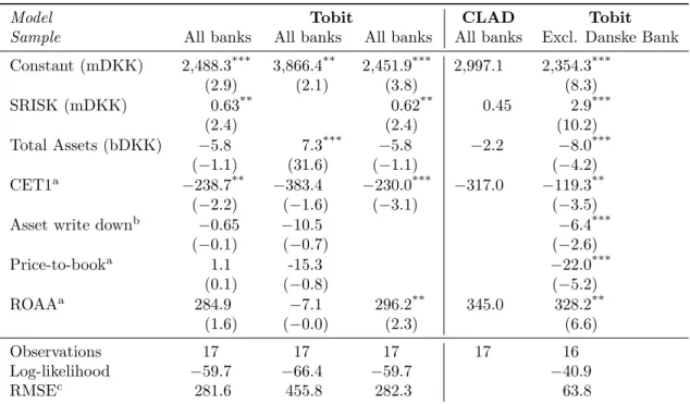
The results from the estimation are stated in Table 4.2. The first column contains the coefficients from the estimated Tobit model including all the control variables. The coefficient on SRISK is positive and significant on a 5 pct. significance level. The value of 0.63 suggests that an increase of 1 mDKK in SRISK predicted an increase of 0.63 mDKK in capital injections under the credit package. It is also worth noting that coefficient on the price-to-book ratio is insignificant suggesting that SRISK is not only a mirror image of the easily available price-to-book ratio. The second column contains coefficients from a Tobit model without SRISK. Interestingly the root mean squared error (RMSE) increases by 60 pct., illustrating how the fit of the model worsens considerably when the information from SRISK is not taken into account. The third column shows the estimated coefficients after removing very insignificant variables one by one, yielding the most compressed
Table 4.2: Capital injections under the credit package and SRISK.
Model Tobit CLAD Tobit
Sample All banks All banks All banks All banks Excl. Danske Bank
Constant (mDKK) 2,488.3*** 3,866.4** 2,451.9*** 2,997.1 2,354.3*** (2.9) (2.1) (3.8) (8.3) SRISK (mDKK) 0.63** 0.62** 0.45 2.9*** (2.4) (2.4) (10.2) Total Assets (bDKK) −5.8 7.3*** −5.8 −2.2 −8.0*** (−1.1) (31.6) (−1.1) (−4.2) CET1a −238.7** −383.4 −230.0*** −317.0 −119.3** (−2.2) (−1.6) (−3.1) (−3.5)
Asset write downb −0.65 −10.5 −6.4***
(−0.1) (−0.7) (−2.6) Price-to-booka 1.1 -15.3 −22.0*** (0.1) (−0.8) (−5.2) ROAAa 284.9 −7.1 296.2** 345.0 328.2** (1.6) (−0.0) (2.3) (6.6) Observations 17 17 17 17 16 Log-likelihood −59.7 −66.4 −59.7 −40.9 RMSEc 281.6 455.8 282.3 63.8
aVariable has been multiplied by 100. Coefficient should be interpreted as change in capital injection (mDKK)
for change of 1 pct. point.
bIn percent of the book value of equity. cRoot mean square error, defined asq1
N
PN
i=1(ˆyi−yi)2, with N being the number of banks and ˆyibeing the
predicted outcome for banki.
Note:Capital injections are in mDKK. Numbers in parenthesies are t-values. ***, ** and * indicate significance on a 1 pct., 5 pct. and 10 pct. level respectively.
model. The coefficient on SRISK is still significant and (even more) positive in this case. All in all, this suggests that SRISK add information over and above what conventional indicators of banks’ health provide when trying to predict the capital injections under the credit package.
As a robustness check, the estimation has also been performed for the compressed model with the less restrictive CLAD-estimator.17 The coefficients are generally in the same range as with the
Tobit model. This suggests that the finding of SRISK having predictive power is robust to the assumptions made when using the Tobit model. Finally, the full model has been estimated on a sample excluding Danske Bank, which, by far, is the biggest purely Danish bank. The coefficient on SRISK increases quite a lot and is still highly significant. All in all, the results lead us to conclude that SRISK at the end of 2008 was a good indicator of the subsequent capital injections that took place during the first half of 2009.
17With the ”censored least absolute deviations” (CLAD) estimator it is only assumed that the median of the error
term conditional on the explanatory variables is 0, cf. Wooldridge (2010). In contrast, the Tobit-estimator assumes that the error terms are independent of the regressors and normally distributed, which can be a harsh assumption. Given the small sample at hand, it is also difficult to test.
4.1.2 What gave rise to changes in SRISK during the financial crisis?
To elaborate on the reason for the capital shortfall during the financial crisis, the evolution in SRISK for Danske Bank (the evolution for the three other financial institutions is illustrated in Figure A.2 in the appendix) is pictured in Figure 4.2 along with the drivers of the change in SRISK. These drivers have been computed by calculating the total differential of SRISK. Note that the market value has been split into the product of the price-to-book ratio (P B) and the book value of equity (E). This is done in order to clearly separate the information obtained from market and accounting data. The parts in bold below are contributions from market data.
dSRISKi,t=k·dDi,t+ (1−k)·PBi,t·Ei,t·dLRMESi,t−(1−k)·(1+LRMESi,t)·Ei,t·dPBi,t
−(1−k)·(1 +LRM ESi,t)·dEi,t·P Bi,t+qmarkett +qt
= debt contribution +LRMES contribution+price-to-book contribution + equity contribution +market cross-effect+ cross-effects.
That is, ignoring the cross-effects18, changes in a firm’s debt, LRMES and market value (stemming
from changes in price-to-book and/or book value of equity) can give rise to changes in its SRISK with weights as stated above. All else equal, higher debt or tail-risk (i.e. a more negative LRMES) increases SRISK while a higher market valuedecreases SRISK.
Figure 4.2: Capital surplus and decomposition of changes for Danske Bank.
Note: Capital surplus is defined as−SRISK. The bars indicate the cumulative contributions from the input variables along with the market cross-effect and a residual, ensuring that the sum of the bars at a given point in
time equals the change in capital surplus from the start of the period. Monthly observations have been used to calculate the contributions. The market is STOXX Europe 600.
The calculated contributions for Danske Bank are stated in Figure 4.2. From a theoretical point of view, the contributions above should be calculated using data with as high a frequency as possible. However, as we have calculated SRISK on a monthly frequency, the contributions have
18The market cross-effect depends on the product of changes in the LRMES and changes in the price-to-book
been approximated using monthly changes in the input variables. Since the residual (which also contains cross-effects) is rather small, we consider the approximation to be reasonable.
Focusing on the change in SRISK for Danske Bank from February 2007 to March 2009 (i.e. from the peak of the capital surplus to the peak in capital shortfall according to SRISK) it appears that changes in the book-to-price ratio and LRMES (”market tail risk”) were the main drivers behind the increase in the capital shortfall, cf. Figure 4.2. Specifically, the decrease in the book-to-price ratio, all else equal, contributed with around 65 pct. of the increase in capital shortfall, the increase in LRMES around 25 pct. and the change in debt around 15 pct. of the increase in the capital shortfall, while an increase in the book value of equity actually decreased the capital shortfall with 5 pct., all else equal. That is, market data was behind the main contribution to the change in SRISK, underlining how SRISK is indeed a market-based stress test. Looking at Figure A.2 in the appendix, one clearly sees how market data also explained the main part of the change in SRISK during the financial crisis for Jyske Bank, Sydbank and Nordea.
4.2
Calculating SRISK for the entire financial sector
Brownlees and Engle (2015) suggest calculating SRISK for the entire financial sector as
SRISKt= N
X
i=1
max (0, SRISKi,t), (13)
where N is the number of financial firms in the Danish financial sector. Equation (13) rests on the idea that financial institutions with capital surpluses will not take over institutions with capital shortfalls in a crisis. That is, capital surpluses cannot compensate for capital shortfalls. The motivation for this is that potential capital shortfalls occur during a crisis, i.e. when the system as a whole is undercapitalized.
Figure 4.3: Total capital surplus and shortfall for Danske Bank, Jyske Bank, Sydbank and Nordea, 2005-2015.
Note: −SRISKis the negative of SRISK as defined in equation (13). The market is STOXX Europe 600.
According to SRISK, the Danish financial sector (note that the entire capital shortfall of the Nordic bank Nordea is included) would have been undercapitalized under stress in February 2008 when Danske Bank began to exhibit a capital shortfall, cf. Figure 4.3. The shortfall gradually grew until March 2009, shortly after the second bank rescue package (the ”credit package”) was adopted
in Denmark. The shortfall decreased (but never became zero) over the following years. With the emergence of the European sovereign debt crisis in 2011, volatility and uncertainty regarding the state of banks and their exposures re-emerged, leading to a sharp increase in the capital shortfall according to SRISK. As Figures 4.2 and A.2 indicate, it was especially changes in the market data that gave rise to the increase in the capital shortfall.
Brownlees and Engle (2015) also suggest calculating the systemicness of a given bank as its share of total SRISK. VLAB19 contains a ranking of international financial institutions according to their share of their region’s SRISK. As illustrated, of the purely Danish banks Danske Bank contributed with the main part of the capital shortfall according to SRISK during the financial crisis.
4.3
Capital shortfall prediction intervals for SRISK
So far, we have calculated LRMES using the average bank return conditional on a market decrease of 40 pct. However, one can also calculate ”percentile-LRMES’s” using percentiles from the return-distribution and subsequently using these for calculating SRISK. The results from doing this are stated in Figure 4.4 for Danske Bank.
Figure 4.4: Capital surplus, prediction interval for Danske Bank.
Note: The numbers, 10, 25, 75 and 90 refer to percentiles of the distribution for LRMES. For instance, the 10-line is−SRISKcalculated using the 10th percentile of LRMES with the other input-variables unchanged.
The leverage ratio is defined as the market value of equity divided with the value of the quasi-assets. The market is STOXX Europe 600.
As illustrated in the figure, the prediction interval for (minus) SRISK for Danske Bank confirms the picture from earlier, with a capital shortfall during both the Financial Crisis of 2007-09 and during the European sovereign debt crisis. There are two factors explaining the dispersion of the SRISK percentiles. The first being the dispersion in the simulated bank-returns conditional on a market decrease (i.e. the dispersion of the observations in Figure 2.2). The second being the market leverage of the bank, i.e. the share of the market value of equity relative to total quasi assets. This is because LRMES ”matters more” when the leverage ratio is high, as a larger share of the assets will adjust in case of a market decrease. This explains why the prediction interval was quite wide just before the financial crisis and today and also why it was so narrow during the financial crisis, where leverage ratios were extremely low.
4.4
Comparing SRISK risk weight with Basel risk weights
Earlier (Section 2.1.8) it was emphasized that only the market’s perception of riskiness of a given financial institution is used in SRISK, no risk weights from either IRB- or standard-methods (”Basel risk weights”) are used. In fact, Acharya et al. (2014) illustrate how a market-based risk weight can be calculated using LRMES. One major advantage of using the market-based risk weights, is that this is derived by looking at the entire portfolio the financial institution has. That is, it takes diversification into account. This is not the case when risk weighting assets using the Basel risk weights, as these are derived in a ”bottom-up” manner by considering asset by asset (Acharya et al. (2014)).
The SRISK risk weight can be derived by using that the capital requirement in SRISK is
SRISKi,t≤0, which enables one to write
SRISKi,t=k·(M Vi,t·(1 +LRM ESi,t) +Di,t)−M Vi,t·(1 +LRM ESi,t)≤0
⇒M Vi,t·(1 +LRM ESi,t)(1−k)≥k·Di,t
⇒M Vi,t·(1 +LRM ESi,t(1−k))≥k·(Di,t+M Vi,t)
⇒M Vi,t ≥
k
1 +LRM ESi,t(1−k)
·Ai,t=RWSRISK·Ai,t.
Hence,RWSRISK can be interpreted as a market-based risk weight, in the sense that it measures
how much equity (measured at market values) a financial institution should use for financing its assets, when taking its estimated crisis-exposure (LRMES) into account.
It would be natural to compare this SRISK-based risk weight with the Basel II risk weights. In Basel II, the risk weights are calculated to reflect the capital needed to cope with a tail scenario so adverse that it covers ”unexpected losses”. Hence, it would be reasonable to compare the SRISK risk weights to the Basel risk weights to evaluate whether there is a common pattern, as the SRISK risk weights also seek to measure risk in an adverse tail scenario.20 To ensure a proper ground of
comparison, only data from after the banks in question moved to IRB-models is considered and the SRISK risk weight is multiplied by 12.5·1.06.21
Figure 4.5 depicts the average Basel risk weight relative to the SRISK risk weight for each quarter from Q3 2008 to Q3 2015, yielding 29 observations for each of the 4 banks. There appears to be a slightly positive relation between the SRISK risk weight and the Basel risk weights for a given bank, while the relation between the Basel and the SRISK risk weight generally appears slightly negative. That is, banks with higher SRISK risk weights appear to exhibit lower Basel risk weights, while changes in Basel and SRISK risk weights over time for a given bank tend to be in the same direction. Using a far larger sample, Acharya et al. (2014) also finds no cross-sectional pattern between Basel and SRISK risk weights. If anything, they find a negative (although insignificant) relation.
As emphasized above, there appear to be rather large differences between the capital requirement in SRISK and the regulatory capital requirement due to the usage of (IRB calculated) risk weights. This would tend to give rise to a different ranking of institutions in need of capital, when using SRISK (or other market-based measures) compared to balance sheet based stress tests. This is also the conclusion in Acharya et al. (2014) who compare the outcome of several of the balance sheet based stress tests performed by US and European regulatory authorities with that of SRISK.
20Note that a 40 pct. decrease over 6 months in STOXX Europe 600 corresponds to the 0.1 percentile when
evaluating from July 1999 to November 2015.
21This is done to ensure that the SRISK risk weight is somewhat comparable to the Basel risk weights. In the
latter case, the capital requirement is multiplied with 12.5 times 1.06 in order to obtain a risk weight (12.5 is the inverse of the minimal capital requirement of 8 pct.), cf. CRD (2013).
Figure 4.5: Comparing average Basel risk weights with SRISK risk weights, 2008-2015.
Note: Average risk weights have been calculated as ”Risk weighted assets” / ”Total assets”. SRISK risk weights have been multiplied by 12.5·1.06.
Source:SNL Financial, Bloomberg and own calculations.
They find no linkage between institutions facing capital shortfalls in SRISK and the stress tests performed by regulatory authorities. Acharya et al. (2014) ascribe this to the fact that regulatory stress tests rely on the usage of the Basel risk weights and that these appear to be uncorrelated with the SRISK risk weights.
In relation to this, Acharya and Steffen (2014b) found that their initial estimates presented in Acharya and Steffen (2014a) of which banks that would need capital under the Comprehensive Assessment did not match the outcome of the Comprehensive Assessment at all. First of all they estimated a total capital shortage using market-based measures that was markedly higher than what was found in the comprehensive assessment. Second, the two tests found that different banks exhibited a capital shortage under stress. Acharya and Steffen (2014b) presented two reasons for these discrepancies, namely that the comprehensive assesment was heavily affected by: ”a) discretion of national regulators in measuring what is ”capital”, and especially b) the use of risk-weighted assets in calculating the prudential capital requirement”(Acharya and Steffen (2014b), p. 4). With point a) referring to e.g. the treatment of goodwill and ”deferred tax assets”.
4.5
Literature on the empirical performance of SRISK
Using Danish data, it has been illustrated that some major Danish banks, under further stress would have exhibited capital shortfalls already in early 2008. It was also found that SRISK would have been useful in predicting which banks that were to apply for capital as part of the credit package in 2009. Looking beyond the borders of Denmark, several other authors have investigated the performance of SRISK in predicting capital shortfalls and systemic risk.
Using US data, Brownlees and Engle (2015) illustrate how firms such as Freddie Mac, Fannie Mae, Lehman Brothers, Bear Stearns and Morgan Stanley according to SRISK exhibited the largest capital shortfalls under stress as early as 1st quarter 2005. All except Morgan Stanley ceased to exist or underwent a substantial restructuring during the financial crisis. Brownlees and Engle (2015) also use SRISK (along with other explanatory variables) to predict the capital injections performed by the Fed during the financial crisis. They find that SRISK significantly improves the ability to predict the capital injections in the US during the crisis.
Looking beyond the financial crisis, Zhang et al. (2015) investigate the performance of four different market-based measures of systemic risk (including ∆CoVaR and SRISK) during three financial crises: the financial crisis of 2007-09, the Asian crisis of 1997 and the Ruble crisis of 1998. Specifically, they investigate whether the four market-based measures under consideration add any early warning signals over and above the signals obtained using conventional risk drivers. They find that ∆CoVaR was the best market-based systemic risk measure at predicting different measures of realized systemic risk (such as realized covariance risk and realized capital shortfall) during the financial crisis of 2007-09. However, Zhang et al. (2015) did not find ∆CoVaR to consistently forecast realized systemic risk during the Asian and Ruble crisis of the late 1990’s. The only market-based measure found to consistently provide regulators with significant early warning signal during all three crises was SRISK, which they found to forecast realized capital shortfall during all three crises. Adding to this, Acharya et al. (2014) find that SRISK is able to rank the institutions in the EBA stress test of 2011 quite well according to their subsequent realized losses.22
Going further back than the abovementioned crises, Brownlees et al. (2015) use a compiled dataset covering US banks from 1866 to 1925, to evaluate the performance of SRISK and ∆CoVaR during multiple banking crises before the introduction of deposit insurance. The authors find that both SRISK and ∆CoVaR are useful in predicting withdrawals of deposits when these led to financial panics, leading them to conclude that the market-based risk-measures are beneficial to regulators.
In sum, the analyses in this paper as well as in Zhang et al. (2015), Acharya et al. (2014) and Brownlees et al. (2015) suggest that SRISK has been able to forecast capital shortfalls during crises (i.e. systemic risk following the definition of Acharya et al. (2012b)) over a long period of time. This indicates that SRISK is indeed a useful measure for regulators when monitoring the vulnerability of the financial sector.
22These results are stated online in Appendix B to their article, see http://www.sciencedirect.com/science/article/pii/S0304393214000725.