Extracting Statistical Graph Features for Accurate and
Efficient Time Series Classification
Daoyuan Li
University of Luxembourg Luxembourg City, LuxembourgJessica Lin
George Mason UniversityFairfax, Virginia, U.S.A. [email protected]
Tegawendé F. Bissyandé
University of Luxembourg Luxembourg City, LuxembourgJacques Klein
University of Luxembourg Luxembourg City, LuxembourgYves Le Traon
University of Luxembourg Luxembourg City, LuxembourgABSTRACT
This paper presents a multiscale visibility graph representation
for time series as well as feature extraction methods for time
se-ries classification (TSC). Unlike traditional TSC approaches that
seek to find global similarities in time series databases (e.g., Near-est Neighbor with Dynamic Time Warping distance) or
meth-ods specializing in locating local patterns/subsequences (e.g., shapelets), we extract solely statistical features from graphs that
are generated from time series. Specifically, we augment time
series by means of their multiscale approximations, which are
fur-ther transformed into a set of visibility graphs. After extracting
probability distributions of small motifs, density, assortativity,
etc., these features are used for building highly accurate clas-sification models using generic classifiers (e.g., Support Vector Machine and eXtreme Gradient Boosting). Thanks to the way
how we transform time series into graphs and extract features
from them, we are able to capture both global and local features
from time series. Based on extensive experiments on a large
num-ber of open datasets and comparison with five state-of-the-art
TSC algorithms, our approach is shown to be both accurate and
efficient: it is more accurate than Learning Shapelets and at the
same time faster than Fast Shapelets.
1
INTRODUCTION
Time series data refer to sequences of data that are ordered either
temporally, spatially or in another defined order. They can be
frequently found in a variety of domains, including financial data
analysis, medical and health monitoring and industrial
automa-tion applicaautoma-tions [27, 28]. Recently, it turns out to be feasible
to model software systems as time series in order to conduct
malware detection and classification [43]. Due to their wide
ap-plication scenarios and abundance, there has been an increasing
need for efficient knowledge discovery methods to extract useful
information from time series databases. One of the major tasks
in time series mining is time series classification (TSC), which
consists of applying a learning algorithm on labeled data to train
a model that will then be used to predict the classes of samples
from an unlabeled data set. Due to the sequential characteristic of
time series data, state-of-the-art classification algorithms (such
as SVM and Random Forest [13]) that perform well for generic
data are generally not suitable for TSC. It is thus important and
beneficial to have a feature extraction mechanism that transforms
© 2018 Copyright held by the owner/author(s). Published in Proceedings of the 21st International Conference on Extending Database Technology (EDBT), March 26-29, 2018, ISBN 978-3-89318-078-3 on OpenProceedings.org.
Distribution of this paper is permitted under the terms of the Creative Commons license CC-by-nc-nd 4.0.
the sequential characteristics of time series data into unordered
feature vectors, so that any modern classification algorithm can
be taken advantage of. After all, one of the most challenging
aspects of TSC lies in the sequentiality property.
Traditionally, researchers often rely on one of the simplest
classifiers for TSC: thekNearest Neighbor (kNN) algorithm. As stated in [6], “all of the current empirical evidence suggests that
simple nearest neighbor classification is very difficult to beat”.
To perform well,kNN classifiers leverage the Dynamic Time Warping (DTW) [7] distance which mitigates problems caused
by distortion in the time axis. One intrinsic issue with DTW,
however, is that it focuses on findingglobalsimilarities,i.e., the overall curveshapeof time series. It also requires applications to specify a proper warping window size or to properly align
data samples. As a result, DTW can be sensitive to data
align-ment/segmentation and it performs better when data are properly
curated. In practice, however, well-aligned time series data are
difficult or expensive to come by [17].
To address the phase issue of DTW- and other
distance-based 1NN approaches, the research community has
pro-posed approaches that focuses on finding defininglocal fea-tures/subsequences in order to be invariant to data alignment
and rotation. Popular methods that fall into this category
in-clude Bag-of-Patterns [31], SAX-VSM [39] and shapelets-based
algorithms [47], such as Fast Shapelets (FS) [35] and Learning
Shapelets (LS) [15]. The majority of these techniques have taken
advantage of text feature extraction approaches –e.g., TF-IDF – after converting time series into alphabetical strings. Such
con-version is often done via Symbolic Aggregate approXimation
(SAX) [30], which requires two parameters (i.e., cardinality and PAA window size) to be set and it may not always be trivial
to find the best pair. Besides, many approaches attempt to find
time series subsequences that are representative of each class,
e.g., shapelets by definition are defining time series subsequences that are calculated by exhaustive or optimized search. Overall,
many of these methods have suffered from high computation
complexity or suboptimal classification accuracy [42].
Graph representations for TSC, on the other hand, have not
been investigated extensively by the time series mining research
community possibly due to their high computation complexity.
Nevertheless, thanks to recent development of graph mining
al-gorithms [5, 33], some of the formerly complex problems can be
solved extremely efficiently with optimization and
paralleliza-tion techniques [2]. Such advances give us the opportunity to
re-evaluate the possibility of taking advantage of graph
repre-sentations and extracting graph features for building an efficient
This paper proposes a novel approach for TSC that considers
time series as complex graphs/networks and extracts from these
networks important statistical features, which are fed to modern
generic classifiers to learn structural knowledge from the original
time series. After evaluating the classification performance with
a large open dataset, we find out that our approach is capable
of making efficient and accurate classification predictions. The
main contributions of this paper are listed as follows:
•We present a multiscale graph representation for time series, so that both global and local features from time
series can be captured, making this approach agnostic
to time series alignment and outperform major
distance-based TSC algorithms.
•Since we transform time series that are intrinsically se-quential into unordered feature vectors, it is then suitable
for taking advantage of modern generic classifiers (e.g., RF, SVM and XGBoost) for efficient feature selection and
clas-sification. This clear separation of feature extraction and
actual classification can help researcher focus on finding
insightful characteristics in time series data without the
need for reinventing the wheel and designing a classifier
from scratch specifically for time series.
•We propose a novel feature extraction and classification method for time series based on calculating probability
distributions of small motifs (i.e., repeated patterns) in vis-ibility graphs and other statistical features such as density,
degree statistics, assortativity and coreness. This feature
extraction mechanism is parameter-free, so that it can be
easy to use and help yield reproducible results.
•We have intentionally chosen a collection of statistical features that are computationally efficient to extract from
graphs and validated their effectiveness in controlled
ex-periments. Moreover, since our feature extraction and
clas-sification process is inherently parallel, it is suitable for
and capable of large scale data explorations.
•After extensively evaluating our approach with a large number of open datasets and comparing with related
re-search efforts, experiment results indeed suggest that
accu-rate and efficient classification can be obtained following
this paradigm.
The remainder of this paper is structured as follows. Section 2
lays down the necessary background. Next, we present our
ap-proach in section 3 and detail TSC accuracy and efficiency
evalu-ation results along with a case study in section 4. For interested
readers, section 5 introduces research work related to ours.
Fi-nally, we conclude the paper with future research directions in
section 6.
2
BACKGROUND
Traditionally, time series refer to a sequence of numbers that are
chronologically ordered. However, in the research community
time series have a much broader scope and do not associate
strictly with timestamps:
Definition 2.1 (Time series). A time series instance T is an ordered sequence of n real-valued variables, i.e., T =
(v1, ...,vn),vi ∈R.
If we consider each point in a time series as a single feature
in a vector, then time series data usually have a huge number
of features. When considering these features as a vector in an
n-dimensional space, time series data are often high dimensional.
Due to difficulties to conduct knowledge discovery tasks on high
dimensional data, it is frequently required to reduce the
dimen-sionality of time series in order to improve computation
effi-ciency:
Definition 2.2 (Dimensionality reduction). The dimensionality of a time series sampleT is the length ofT, denoted by|T|. IfT′ is an approximated representation ofTand|T′| ≪ |T|, thenT′ is a dimension-reduced representation ofT.
The research community has proposed a number of
dimension-ality reduction techniques for time series, including sampling,
Wavelet transform [25, 26], Piecewise Aggregate Approximation
(PAA) [19],etc.. Among them PAA is perhaps one of the sim-plest and most widely applied approaches. PAA reduces time
seriesT = (v1, ...,vn)fromndimensions tosdimensions by firstly dividing the data intossegments of equal size, then the approximation is a vector of the mean values of the data readings
per segment [30]. LetT′=(v′
1, ...,v ′
s)be this vector wherevi′is computed by equation 1. For the sake of simplicity, n
s is often chosen to be an integer or rounded to the nearest one.
v′ i =ns n si Õ k=n s(i−1)+1 vk (1)
One of the core routines in distance-based classification
al-gorithms involves evaluating the dissimilarity (or similarity) of
two time series. There are a number of dissimilarity measures
for time series, two of the most frequently used measures in the
research community are Euclidean distance and DTW distance.
The Euclidean distance maintains a one-to-one mapping of all
the points in two series. On the other hand, the DTW distance
tries to find the best mapping of points in two series using the
dynamic programming paradigm, so that the minimum distance
between these two series is achieved. The paradigm is called
“time warping” since the time axis of series can be expanded or
compressed in order to ensure the minimum distance,i.e., anith point inXcan be mapped to ajthpoint (it is possible thati,j), or one point inX may even be mapped to multiple points inY.
2.1
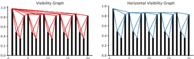
Visibility Graph
Aiming for taking advantage of graph theories as a way of
characterizing time series, an algorithm named visibility graph
(VG) [22, 23] is proposed to transforms time series into a network
structure. The creation of VGs relies on an extremely simple idea:
each point in a time series is treated as a vertical bar, whose
height is the corresponding numerical value. When considering
these bars on a landscape, it is then straightforward that the
top of a bar may be visible from the top of other bars. Assume
each time-step as a vertex in a graph, then two vertices are
con-nected if the top of the vertical bars are visible to each other,i.e., there exists a straight line from the top of the two bars without
intersecting with other bars. More formally,
Definition 2.3 (Visibility graph). Given a time seriesT =
(v1, ...,vn), its VG representationG = (V,E) hasn vertices: V = (1, ...,n). An edgee =(i,j) ∈Eiff∀ksuch thati <k <
j(1≤i,j≤n)inequalityvk<vj+(vi−vj)jj−−ik is satisfied. It is obvious that VGs are undirected, although it is possible
to create a directed version by limiting the direction of
view-points from the vertical bars. Besides, VGs are always connected
0 5 10 15 20 0.0 0.2 0.4 0.6 0.8 1.0 Visibility Graph 0 5 10 15 20 0.0 0.2 0.4 0.6 0.8
1.0 Horizontal Visibility Graph
Figure 1: An example of converting time series to visibility graph and horizontal visibility graph.
VGs are invariant when time series undergo affine
transforma-tions,i.e., the visibility criterion remains fulfilled when rescaling the time series either horizontally or vertically. However, VGs
are not suitable for non-stationary time series,i.e., those hav-ing monotonically increashav-ing/decreashav-ing trends in time. Such
trends should be removed before applying VG generation. The
goal of VGs is to characterize structural properties [23] of time
series, such as periodicity, fractality,etc., although it is shown that it can be extended to weighted VGs in order to quantitatively
distinguish generic time series [41].
Creation of VGs from time series without optimization
gener-ally hasO(n2)computation complexity, wherenis the dimension-ality of time series data. However, a more efficient VG generation
algorithm [1] can have a sub-quadratic computation complexity.
Specifically, this algorithm can reduce the complexity of time
series VG generation down toO(nlog2(n)). When further taking advantage of parallelization,O(nlog2(n))work can be effectively solved withinO(log2(n))time. Another simplified variant of VG, horizontal visibility graph (HVG) [32], only connects nodesiand
jif a horizontal line can be drawn between these nodes. Creation of HVGs without any optimization generally has a computation
complexity ofO(n).
Definition 2.4 (Horizontal visibility graph). Given a time series
T =(v1, ...,vn), its HVG representation ¯G=(V,E)hasnvertices: V =(1, ...,n). An edgee =(i,j) ∈ Eiff∀ksuch thati <k <
j(1≤i,j≤n)inequalityvi,vj >vkis satisfied.
VG and its variants have been shown to be able to differentiate
certain time series. For instance, [18] have extracted motifs from
HVGs and claimed the motif statistics can be used for
differenti-ating various types of time series data, including white Gaussian
noises, fully chaotic logistic maps and noisy fully chaotic logistic
maps. The authors further claimed that HVG motif profiles from
heart rate time series can be used to cluster different types of
meditative activities.
Intuitively, VGs and HVGs are very similar concepts and HVG
is a subgraph of VG. However, when extracting statistics from
them, VGs can be more capable of capturing global features,
while HVGs are often more sensitive to local variations. As a
result, VGs and HVGs can be joined to provide more accurate
representations of time series data. We will discuss more about
such heuristics in section 4.2. For simplicity, in the remainder
of this paper the term VG indicates the combination of VG and
HVG if HVG is not explicitly specified.
2.2
Graph Features
Extracting features from graphs has become a popular research
topic thanks to the recent applications in social network
anal-ysis, physics as well as bio-informatics. There are a number of
research avenues in graph mining, the most popular ones are
about finding communities or clusters within large graphs and
characterizing graphs by means of finding and counting
recur-rent patterns. Since time series VGs are always connected, it is
thus not immediately helpful to extract clusters, since clusters in
these graphs will always correspond to subsequences of original
time series. Graph motifs or graphlets, however, are especially
interesting since they are sub-graph structures or patterns in a
larger graph that are recurrent and statistically significant.
Find-ing motifs in graphs is generally a complex problem, but there
have been a number of research work for efficiently extracting
motifs from graph data, such as GTrieScanner [37] and Parallel
Parameterized Graphlet Decomposition (PGD) [2]. Due to the
fact that the number of motifs increases exponentially with
mo-tif size, the complexity of finding momo-tifs is also exponentially
correlated with motif size. Researchers thus generally focus on
optimizing computation efficiency of locating small motifs (of
size up to four). PGD is the state-of-the-art approach for
effi-ciently finding and counting small motifs in graphs and can be
several magnitudes faster than other approaches. Table 1 shows
all possible small graph motifs up to size four. Note that PGD
works only for undirected graphs, while GTrieScanner works on
both directed and undirected graphs. However, motifs extracted
by GTrieScanner are only connected motifs and the running time
is significantly slower than PGD. As a result, in this paper we
take advantage of PGD for small motif counting.
Table 1: All graph motifs up to size 4. Note that connected graphs may contain disconnected motifs.
# Motif Name # Motif Name
M21 2-edge M22 2-node-independent M31 3-triangle M33 3-node-1-edge Connected M32 3-path Disconnected M34 3-node-independent M41 4-clique M47 4-node-triangle M42 4-chordal-cycle M48 4-node-star M43 4-tailed-triangle M49 4-node-2-edges M44 4-cycle M410 4-node-1-edge M45 4-star M411 4-node-independent M46 4-path
Researchers argue that motif distribution extracted from VGs
can be extremely helpful for identifying different types of
artifi-cially generated time series. However, in practice motif
distribu-tions may not be as distinguishable as those from artificial data.
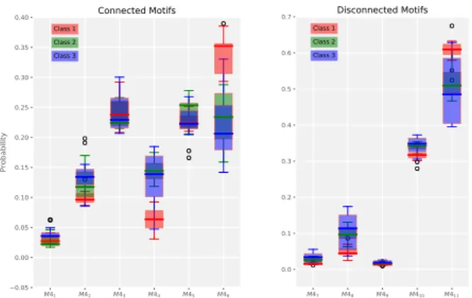
For example, Figure 2 illustrates the motif distributions of three
different classes of time series from theArrowHeaddataset. As shown, it can be very difficult to tell one class apart from another
given only these distributions since the probability distributions
of different classes tend to overlap, especially in this case for
instances from class 2 and 3. Besides small motifs, other graph
features are also easy to obtain,e.g., vertex and edge statistics as well as structural metrics. In this paper we consider some
additional graph features listed as follows:
• Density: the ratio of the number of edges to the number of all possible edges. Graph density is computed following
equation 2 and has a computation complexity ofO(1).
p=|V|(|2V|E| −| 1)
(2)
• K-core: theK-core of a graphG =(V,E)is a maximal subgraphH =(V′,E′)in which each vertex has a degree of at leastK,i.e.,∀v ∈V′: degH(v) ≥K. Consequently, it is a cohesiveness measurement of interlinked subgraphs
M41 M42 M43 M44 M45 M46 0.05 0.00 0.05 0.10 0.15 0.20 0.25 0.30 0.35 0.40 Probability Class 1 Class 2 Class 3 Connected Motifs M47 M48 M49 M410 M411 0.0 0.1 0.2 0.3 0.4 0.5 0.6 0.7 Class 1 Class 2 Class 3 Disconnected Motifs
Figure 2: Boxplots of motif probability distribution of different classes from the ArrowHead Dataset’s training set.
within a network andKis computed by equation 3. Com-putingKhas anO(|E|)time complexity [5].
K=arg max
H∈GCoreH ≥K (3)
•Assortativity coefficient: a metric to measure the correla-tion of vertices in a graph through calculating the Pearson
correlation coefficient of degree between pairs of
con-nected vertices. Equation 4 shows how assortativity
coef-ficient is computed, r= Í xyxy(exy−axby) σaσb (4)
whereaxandbyrepresents respectively the fraction of edges that start and end at vertices with valuesxandy, and
exyis the measure of assortativity, such thatÍxyexy =1,
Í
yexy = ax andÍxexy =by. Finally,σaandσb are the standard deviations of the distributionsax andby. Computingrhas anO(|E|)time complexity [33].
•Degree statistics including max, min and mean degree per vertex. Naturally, computing such statistics has anO(|V|) time complexity.
Note that there are a plethora of features that can be extracted
from graphs [11], and such features are not necessarily equally
easy to obtain. For instance, the diameter of a graph – which is
the shortest distance between the two most distant vertices in the
graph – can be computationally expensive to calculate since it
demandsO(|V|(|V|+|E|))computation. Nonetheless, this paper does not intend to find the exclusive set of features that are both
efficient and descriptive for time series VGs. Rather, we try to
investigate if these aforementioned statistical features are indeed
helpful for TSC.
3
MULTISCALE VISIBILITY GRAPH
Time series data differ greatly in characteristics depending on
how they are captured, sampled and their underlying
applica-tions: in one domain global features may be helpful, while in
another domain local features (i.e., defining subsequences) can become more important for classification. After transforming
real-valued time series into VGs, specific features from such VGs
– such as probability distributions of small motifs – are more
re-flective of local features than global ones. We refer to this type of
representation as Uniscale Visibility Graph (UVG) in the
remain-der of this paper. In this case, extracting more global features
(i.e., probability distributions of large motifs) becomes exponen-tially expensive for computation. To mitigate this problem, we
propose the Multiscale Visibility Graph (MVG) representation
such that each time series sequence is transformed into a set of
dimensionality-reduced approximations: these downscaled
ap-proximations are then converted into a set of VGs. Consequently,
features are extracted from each graph in MVGs, thus
approxi-mating the process of extracting features of different scales. This
approach is inspired by computationally efficient wavelet
trans-form [10], with the exception that time series in each scale are
represented with graph structures instead of numerical values.
We first define the multiscale representation of time series as
follows:
Definition 3.1 (Multiscale Approximation). Given a time series
T0=(v1, ...,vn), its approximated multiscale representation is a
set of time seriesTˆ=(T1,T2, , ...,Tm), whereTi (1≤i≤m) is a
downscaled approximation ofT0, such that|Ti|=|T0|/2i =n/2i.
In addition, to avoid tiny and meaningless representations we
en-force a constant thresholdτfor the downscaled approximations,
i.e.,|Tm|>τ.
The downscaling ofT0can be achieved with widely used
di-mensionality reduction techniques such as PAA (cf.equation 1). Since the size of downscaled time series representations follows
an exponential decay, time series multiscale representationsTˆ often consists of a small number downscaled series. Besides,
con-sideringÍ∞i
=1n∗2
−i =n, theoretically the maximal dimension
ofTˆwhen fully expanded isn.
Definition 3.2 (Multiscale representation). Given a time se-riesT0 and its approximated multiscale representation Tˆ =
(T1,T2, , ...,Tm), its multiscale representation is the union of
ˆ
T
andT0,i.e.,T=(T0,T1,T2, , ...,Tm).
Approximated multiscale representations can help smoothing
time series and reducing noises, while full multiscale
represen-tations consist of both the original time series and augmented
versions. Each series in multiscale representations can be
trans-formed into VGs, thus we have a natural definition for multiscale
visibility graphs, which are supersets of approximated multiscale
visibility graphs (AMVGs):
Definition 3.3 (Multiscale visibility graph). Given a time se-riesT and its multiscale representationT=(T0,T1,T2, , ...,Tm),
its multiscale visibility graph is a set of graphs G =
(G0,G1,G2, , ...,Gm), whereGi (1≤i≤m) is the corresponding
visibility graph created fromTi.
Since the number of vertices inGiequals the dimensionality ofTi, to avoid meaningless trivial graphs it is natural to setτ to a small integer (e.g.,τ = 15), such that the smallest graph inGcontains more thanτvertices. Note thatτshould not be considered as a parameter for the feature extraction process.
Rather, it is more an optimization trick and bearing a default
value of 0 will not cause any issues, since feature selection is
done during classification.
3.1
Feature Extraction
As shown in Algorithm 1, feature extraction in MVGs follow
the same paradigm as extracting features from individual graphs
in an MVG and concatenating all features together, since graph
features extracted in this paper are solely statistical and do not
pertain orders. Consequently, these features can be fed into any
generic classification algorithms [13] well studied in the machine
learning and data mining community. It is utterly important that
of time series data into unordered feature vectors, so that any
modern classification algorithm can be taken advantage of.
Algorithm 1Building time series MVGs and extracting features
from them.
1:procedureExtractFeatures(T)
2: F← ▷Feature set
3: G← ▷MVGs
4: T′←T
5: while|T′|>τdo ▷Ignore trivial graphs
6: G←G∪BuildV GAndHV G(T′)
7: T′←DimensionalityReduction(T) ▷|T′| ≤|T|
2
8: forG∈Gdo
9: M←Motif ProbabilityDistr ibution(G) 10: M←N ormalize(M)
11: F←F∪ {M,Other Statistics(G)}
12: returnF
Although features have become unordered, it is nevertheless
important to carefully curate them in order to achieve better
classification results. Note that PGD is very efficient in counting
motifs in graphs, and the dominant features from time series
MVGs will be the probability distribution of motifs of different
sizes:
Definition 3.4 (Motif probability distribution). Given a time series visibility graphGand the set of motifsM, the motif proba-bility distributionPGis the set of probabilities corresponding to each motif inM.
Empirically, the distribution of connected and disconnected
motifs vary greatly in graphs. It is thus desirable to calculate
separately motif probability distributions depending upon motif
connectivity. To that end, the motif probability distributions
(MPDs) are calculated per motif size and connectivity. This
es-sentially normalizes extracted motif features. Specifically, MPDs
are normalized according to the following five groups (cf.Table 1):
{{M21,M22},{M31,M32},{M33,M34},{M41, ...,M46},{M47, ..., M411}}. Finally, it is obvious that other graph features –e.g.,
graph density and assortativity coefficient – are independent
of MPDs. As a result, no further curation for such features is
needed.
3.2
Classification
When features are extracted, we can feed them into a generic
classifier to learn from labeled samples and predict the class of
unlabeled ones. We are in favor of most well-known and widely
accepted and well optimized algorithms such as SVM, Random
Forest and eXtreme Gradient Boosting (XGBoost) [8] for this
task. Especially, as a highly optimized distributed gradient
boost-ing library, XGBoost runs on major distributed environment. It
has gained remarkable adoption since its inception and is well
known for its performance in machine learning and data mining
competitions.
Typical classification tasks involve learning models and
se-lecting a performant estimator through the process of
valida-tion. Although in this study we have proposed a parameter-free
method for feature extraction, it is still required to tune the
hyper-parameters for generic classifiers. Note that hyper-hyper-parameters
in machine learning refers to parameters that are external to the
model and such values cannot be estimated from the training
data. As a result, they are often set using heuristics. For instance,
thekinkNN classifier can be considered as a hyper-parameter, since “there is no analytical formula available to calculate an
appropriate value” [21]. In order to tune hyper-parameters in
our classifiers, we conduct cross-validation to evaluate the
per-formance of estimators and apply grid search to find the most
satisfactory estimator based on the cross entropy scores:
−logP(yˆ|y)=−(ylog(yˆ)+(1−y)log(1−yˆ)) (5) whereyis the ground truth, and ˆyis the probabilistic predic-tions by an estimator. Since datasets may be highly imbalanced,
which will lead to degraded classification results, we can apply
random oversampling techniques over the minority class and
use stratified cross validation to preserve class balance when
validating models.
4
EVALUATION
To evaluate our approach, we conduct experiments using a large
number of publicly accessible datasets. We first introduce the
datasets. Then we list and validate our heuristics, followed by
creating an accurate classifier with stacked generalization. Next,
we compare the accuracy and efficiency of our method with
state-of-the-art approaches. Finally, we close this section with a case
study and discussions.
4.1
Datasets
When validating our heuristics, we consider the most popular
and largest open dataset for TSC: the UCR Time Series
Classifi-cation Archive [9]. Specifically, we use a subset from the UCR
archive that are more recent (added after the summer of 2015),
which include datasets from various fields ranging from
elec-trocardiograms (ECG) to intra-species image recognition data.
These datasets have a uniform file format and consistent internal
data structures, making it possible to conduct batch processing in
a content-agnostic manner. Furthermore, datasets in this subset
are generally larger in size, making it more reliable to evaluate
the scalability of TSC algorithms.
When comparing our approach with state-of-the-art
ap-proaches, we take advantage of the UEA & UCR Time Series
Classification Repository since it contains all datasets from the
UCR archive. In addition, this repository also provides open
source implementation for more than 18 TSC algorithms [3]
and benchmarking results are publicly available from the
reposi-tory website1. We compare our results with relevant algorithms using the default train and test split from this repository.
4.2
Validating Heuristics
Before diving directly into MVG representations, it would be a
prerequisite to validate our heuristics step by step. We summarize
these heuristics below:
(1) Motif statistics from VGs and HVGs can serve better
dur-ing classification when combined with other graph
fea-tures such as degree statistics.
(2) Features from HVGs are more capable of capturinglocal characteristics while those from VGs are capable of
captur-ingglobalcharacteristics. Combining features from both HVGs and VGs can help yield more accurate classification
results.
(3) Multiscale representations are able to reveal time series
features at different scales, and a generic classifier is able
to conduct feature selection and find important features to
perform more accurate classification than using features
without multiscale augmentation.
1
When validating these heuristics, we feed the features
corre-sponding to each heuristic to an XGBoost classifier for 3-fold
cross-validation and model selection. A set of hyper-parameters
have been set for grid search, including the learning rate (three
choices from 0.01 to 0.3), number of estimators (10 choices from
10 to 100), max tree depth (10 or 20). In order to prevent
overfit-ting, the subsampling and column sampling hyper-parameters
are both set to 0.5 to randomly collect half of the data instances
and features to grow trees. To reduce the impact of random over
sampling on minority classes and floating-point summation
is-sues in parallel processing, all experiments have been repeated
five times and average accuracy scores are calculated. Finally,
all experiments are conducted on a Linux server with two Intel
Xeon E5-2430 CP Us with a clock rate of 2.20GHz. With this setup,
we illustrate step by step how experiments are setup and present
the final classification results in Table 2.
4.2.1 Choosing Graph Features. We first investigate which
graph features are helpful for extracting distinguishable
informa-tion from time series. Specifically, we transform time series into
UVGs consisting of both VG and HVG representations and try
to extract MPDs as well as other features (density, assortativity
and degree statistics) from these graphs. We are interested in
finding out whether MPDs are sufficient for TSC and if
extract-ing other statistic features from graphs are necessary. Next, we
take advantage of XGBoost classifier to train on different feature
sets and classify the test datasets. Columns A, B, C and D in
Table 2 presents the classification error rates using HVG with
only MPDs, HVG with MPDs and other graph features, VG with
only MPDs and VG with all features. Comparison on the bottom
of the table shows that including features such as density and
assortativity coefficient indeed helps improving classification
ac-curacy. For HVGs, including features other than MPDs increases
classification accuracy in 32 datasets, while for VGs 29 datasets
saw accuracy improvements. A Wilcoxon signed rank test with
p-values9.48e-7and9.56e-5suggests that such improvement is indeed significant (bothp-values < 0.05). Figure 3 shows the clas-sification results in the form of scatter plots, where each point
represent a dataset. Such results along with the Wilcoxon test
indeed suggest that our Heuristic (1) is valid.
0.0 0.2 0.4 0.6 0.8 0.0 0.2 0.4 0.6 0.8 HVG MPDs wins HVG Allwins HVG MPDs vs. HVG All 0.0 0.2 0.4 0.6 0.8 0.0 0.2 0.4 0.6 0.8 VG MPDs wins VG All wins VG MPDs vs. VG All
Figure 3: Comparison of classification error rates: using MPDs with or without other graph features.
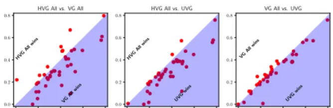
4.2.2 VG and HVG.Next, it is necessary to show that graph
features extracted from both VGs and HVGs are important. Recall
that, intuitively, VGs are helpful for capturing global features
while HVG can help locating local features. We separately test the
distinguishing power of VGs and HVGs for time series in order to
make sure that both can lead to satisfactory classification results.
Furthermore, we conduct experiments to investigate if combining
VGs and HVGs can better capture both global and local features
for time series and thus lead to more accurate classification.
Figure 4 illustrates the comparison of classification accuracy
with VG and HVG features as well as combining both VG and
0.0 0.2 0.4 0.6 0.8 0.0 0.2 0.4 0.6 0.8 HVG All wins VG All wins HVG All vs. VG All 0.0 0.2 0.4 0.6 0.8 0.0 0.2 0.4 0.6 0.8 HVG All wins UVG wins HVG All vs. UVG 0.0 0.2 0.4 0.6 0.8 0.0 0.2 0.4 0.6 0.8 VG Allwins UVG wins VG All vs. UVG
Figure 4: Comparison of classification error rates: using HVGs, VGs or combining two together (denoted as UVG here).
HVG. The first scatter plot shows that for majority datasets,
VG features can yield more accurate classification performance.
However, it is still worth mentioning that HVG features can also
outperform VG features in some specific datasets, possibly due
to the reason that local features are more influential in such
datasets. Moreover, it is obvious from the other two scatter plots
in Figure 4 that combining both VG features and HVG features
can greatly boost the classification accuracy. This is probably
due to the excellent feature selection capability of XGBoost, so
that the classifier is able to find out which features are more
important during the training process. In addition, as shown in
Table 2, using VGs outperforms HVGs in 30 datasets with ap -value of3.09e-3, suggesting VGs are capable of capturing more characteristics in time series. Finally, combining features from
both VGs and HVGs yields more accurate results in 27 datasets
with ap-value of5.01e-3, indicating significant improvement when combining two different types of graphs. As a result, the
validity of our Heuristic (2) can be confirmed.
4.2.3 UVG, AMVG and MVG. Since we have demonstrated
that taking advantage of both VG and HVG features can improve
classification accuracy for UVG representations, now we can
investigate whether Heuristic (3) holds,i.e., if multiscale repre-sentations can help achieving even more accurate results. To
visually inspect which representation suites best for TSC, we
further draw scatter plots of the accuracy results in Figure 5. It is
then obvious that AMVG and UVG (scatter plot on top) lead to
similar classification accuracy, which suggests that AMVG can be
good approximations for original time series data. Furthermore,
the two scatter plots in the bottom of Figure 5 indeed confirm that
MVG representations result in better classification performance,
since almost all dots representing results from different datasets
fall on the side of MVG.
0.0 0.2 0.4 0.6 0.8 0.0 0.2 0.4 0.6 0.8 UVG wins AMV Gwins UVG vs. AMVG 0.0 0.2 0.4 0.6 0.8 0.0 0.2 0.4 0.6 0.8 AMV Gwins MVG wins AMVG vs. MVG 0.0 0.2 0.4 0.6 0.8 0.0 0.2 0.4 0.6 0.8 UVG wins MVG wins UVG vs. MVG
Figure 5: Comparison of UVG, AMVG and MVG’s error rates.
From Table 2, we can see that multiscale approximations
out-performs uniscale time series in 19 datasets, with a Wilcoxon
p-value of0.8623> 0.05. As a result, AMVG representations are not statistically significantly different than UVGs. On the other
hand, MVGs outperform AMVG in 29 datasets with ap-value of
1.72e-4and MVGs are more accurate than UVGs in 30 datasets with ap-value of8.74e-4, suggesting that MVG representations indeed contribute significantly towards a more accurate feature
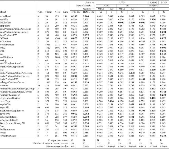
Table 2: Error rates of classifying 39 UCR datasets compared with 1NN-Euclidean and 1NN-DTW. Different heuristic combinations are taken into account. Bold-faced values indicate lowest error rates (including ties) for specific datasets in all experiments.
Scales→ UVG AMVG MVG
Type of Graphs→ HVG VG VG+HVG
Features→ MPDs All MPDs All All
Dataset #Cls. #Train #Test Dim. 1NN-ED 1NN-DTW A B C D E F G
ArrowHead 3 36 175 251 0.200 0.200 0.482 0.449 0.406 0.407 0.385 0.405 0.398 BeetleFly 2 20 20 512 0.250 0.300 0.440 0.410 0.250 0.170 0.250 0.150 0.180 BirdChicken 2 20 20 512 0.450 0.300 0.260 0.150 0.000 0.000 0.000 0.050 0.050 Computers 2 250 250 720 0.424 0.380 0.294 0.284 0.367 0.338 0.281 0.292 0.266 DistalPhalanxOutlineAgeGroup 3 139 400 80 0.218 0.228 0.204 0.202 0.214 0.196 0.202 0.196 0.188 DistalPhalanxOutlineCorrect 2 276 600 80 0.248 0.232 0.409 0.389 0.251 0.263 0.251 0.264 0.231 DistalPhalanxTW 6 139 400 80 0.273 0.272 0.342 0.348 0.298 0.300 0.315 0.275 0.279 ECG5000 5 500 4500 140 0.075 0.075 0.289 0.182 0.137 0.112 0.116 0.076 0.075 Earthquakes 2 139 322 512 0.326 0.258 0.262 0.255 0.286 0.265 0.245 0.276 0.283 ElectricDevices 7 8926 7711 96 0.450 0.376 0.503 0.493 0.392 0.357 0.366 0.368 0.338 FordA 2 1320 3601 500 0.341 0.341 0.009 0.009 0.254 0.220 0.007 0.167 0.006 FordB 2 810 3636 500 0.442 0.414 0.328 0.318 0.313 0.290 0.271 0.257 0.230 Ham 2 109 105 431 0.400 0.400 0.463 0.463 0.347 0.345 0.389 0.389 0.343 HandOutlines 2 370 1000 2709 0.199 0.197 0.293 0.288 0.275 0.225 0.221 0.215 0.206 Herring 2 64 64 512 0.484 0.469 0.425 0.419 0.450 0.484 0.381 0.431 0.288 InsectWingbeatSound 11 220 1980 256 0.438 0.422 0.808 0.763 0.586 0.577 0.557 0.484 0.488 LargeKitchenAppliances 3 375 375 720 0.507 0.205 0.461 0.414 0.490 0.478 0.380 0.346 0.325 Meat 3 60 60 448 0.067 0.067 0.497 0.490 0.160 0.097 0.117 0.050 0.080 MiddlePhalanxOutlineAgeGroup 3 154 400 80 0.260 0.253 0.274 0.279 0.246 0.238 0.267 0.266 0.247 MiddlePhalanxOutlineCorrect 2 291 600 80 0.247 0.318 0.534 0.531 0.305 0.294 0.337 0.426 0.314 MiddlePhalanxTW 6 154 399 80 0.439 0.419 0.471 0.443 0.419 0.426 0.401 0.434 0.410 PhalangesOutlinesCorrect 2 1800 858 80 0.239 0.239 0.397 0.391 0.302 0.291 0.288 0.272 0.264 Phoneme 39 214 1896 1024 0.891 0.773 0.798 0.786 0.812 0.797 0.759 0.772 0.730 ProximalPhalanxOutlineAgeGroup 3 400 205 80 0.215 0.215 0.207 0.194 0.185 0.192 0.178 0.152 0.170 ProximalPhalanxOutlineCorrect 2 600 291 80 0.192 0.210 0.280 0.267 0.167 0.165 0.174 0.181 0.144 ProximalPhalanxTW 6 205 400 80 0.292 0.263 0.303 0.307 0.257 0.259 0.257 0.300 0.233 RefrigerationDevices 3 375 375 720 0.605 0.560 0.533 0.523 0.526 0.494 0.478 0.415 0.417 ScreenType 3 375 375 720 0.640 0.589 0.506 0.486 0.678 0.669 0.572 0.506 0.499 ShapeletSim 2 20 180 500 0.461 0.300 0.189 0.194 0.067 0.051 0.017 0.161 0.047 ShapesAll 60 600 600 512 0.248 0.198 0.715 0.595 0.585 0.485 0.448 0.332 0.313 SmallKitchenAppliances 3 375 375 720 0.659 0.328 0.239 0.212 0.282 0.261 0.205 0.205 0.206 Strawberry 2 370 613 235 0.062 0.062 0.217 0.205 0.117 0.113 0.097 0.099 0.094 ToeSegmentation1 2 40 228 277 0.320 0.250 0.354 0.339 0.289 0.301 0.296 0.261 0.259 ToeSegmentation2 2 36 130 343 0.192 0.092 0.185 0.185 0.205 0.182 0.185 0.218 0.185 UWaveGestureLibraryAll 8 896 3582 945 0.052 0.034 0.551 0.498 0.516 0.482 0.386 0.278 0.265 Wine 2 57 54 234 0.389 0.389 0.493 0.404 0.530 0.519 0.448 0.556 0.548 WordSynonyms 25 267 638 270 0.382 0.252 0.794 0.770 0.662 0.610 0.578 0.559 0.571 Worms 5 77 181 900 0.635 0.586 0.492 0.470 0.414 0.409 0.387 0.448 0.409 WormsTwoClass 2 77 181 900 0.414 0.414 0.328 0.306 0.242 0.248 0.243 0.239 0.233 Comparison versus G G B D D E F G E
Number of more accurate datasets 26 23 32 30 29 27 19 29 30 Wilcoxon testp-value 0.01 0.1638 9.48e-7 3.09e-3 9.56e-5 5.01e-3 0.8623 1.72e-4 8.74e-4
4.2.4 Summary of Heuristic Validation. Overall, all our
heuris-tics are supported by experiment results and each heuristic
con-tributes significantly to a more accurate TSC process. Table 2
also shows the comparison between our approach and Euclidean
distance- as well as DTW-based nearest neighbor classification.
Our approach outperforms 1NN-Euclidean in 26 datasets with a
Wilcoxonp-value of0.01, suggesting MVG features with XGBoost is significantly more accurate than 1NN-Euclidean. Moreover,
MVG appears to be in par with 1NN-DTW in terms of
classifi-cation accuracy since 23 datasets are in favor of MVG with a
p-value of0.1638. Next, we will try to build a more robust and accurate classifier using stacked generalization.
4.3
Stacked Generalization
Previously we have solely taken advantage of XGBoost for
classi-fying time series with features extracted from graphs. However,
it can also be interesting to investigate if other classifiers can
achieve similar results. Besides, although modern classifiers such
as XGBoost and RF are capable of efficiently conducting feature
selection during training, we can still conduct feature selection
processes and feed sucha prioriinformation to classifiers in order to achieve better classification accuracy. To that end, we propose
feeding different sets of features to a collection of classifiers and
then create a meta-classifier using stacked generalization (a.k.a stacking or blending) [44]. This meta-classifier will then
hope-fully generate better final predictions. In fact, a variant of this
technique has led to winning the Netflix Prize with a reward of
one million dollars [40].
Before building a meta-classifier with stacked generalization,
we first make sure that features we previously extracted are
suit-able inputs for different classifiers such as RF and SVM. Generally,
tree-based classifiers are not so sensitive to monotonic
transfor-mations of individual features. As a result, it is often not required
to have features scaled to similar magnitudes for RF and XGBoost.
However, since SVM’s kernel functions (in an Euclidean space)
are usually sensitive to different feature magnitudes, we use
Min-Max scaling to transform each feature into range of zero and one.
After that, we compare the classification performance of these
In order to evaluate the significance of the differences a generic
classifier can incur, we take advantage of the Nemenyi test [12],
which is a post-hoc test aiming for finding whether groups of
data differ after a statistical test of multiple comparisons. This
test can be illustrated by means of a critical difference diagram,
where average ranks of all approaches are presented. Specifically,
the location of vertical lines indicate the average ranking of an
approach and bold lines (insignificance lines) indicate groups of
approaches that are not significantly different. In this case, for one
approach to be considered significantly better than another, its
overall ranking has to be at least 0.5307 higher than its competitor. As shown in Figure 6, XGBoost performs slightly better than
RF in general, and both are significantly more accurate than
SVM. Such results are not surprising, since [13] have empirically
tested hundreds of classifiers and concluded that RF produces the
most accurate classification results. This study was conducted
before the initial release of XGBoost, and the recent adoption
momentum of XGBoost indeed suggests that XGBoost is great
for yielding accurate classification results.
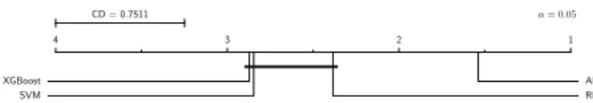
1 2 3 MVG (SVM) MVG (RF) MVG (XGBoost) CD = 0.5307 ↵= 0.05
Figure 6: Critical difference diagram comparison of RF, SVM and XGBoost.
Now that generic classifiers can be used for graph features
extracted from time series, we then set to investigate whether
stacking can help further increase classification accuracy. We first
stack top performing classifiers in each family before blending
classifiers from different families. Specifically, we first select the
top five most accurate classifiers from RF, SVM and XGBoost
through cross validation. Then these five classifiers are stacked
to produce a meta-classifier, which is used for producing final
predictions. Finally, when stacking classifiers of different families,
five classifiers from each family have been selected, thus the
meta-classifier has been trained with 15 meta-classifiers. Our algorithm is
described in Algorithm 2.
Algorithm 2Algorithm for creating an ensemble classifiers
us-ing stacked generalization.
Input:Training datasetD={Xi,yi}mi=
1(Xi∈R
n,yi∈
Z)
Base classifiersH(with different hyper-parameters)
Output:An stacked ensembleE
1:procedureBuildStackingEnsemble(D,H)
2: S←CreateStratifiedKFolds(D, cv=3) ▷3-fold CV 3: E← ▷Best performing base estimators
4: for allh∈Hdo
5: H←
6: for allS={Dt r ain,Dval idat ion} ∈Sdo
7: TrainClassifier(h,Dt r ain) 8: yˆ←Predict(h,Xval idat ion) 9: score← −logP(yˆ|yval idat ion)
10: H←H∪ {h,scor e}
11: H←arg sort(H) ▷Sort estimators by score 12: E←E∪slice(H,k) ▷Select top-kestimators 13: W ←ComputeEstimatorWeights(E) ▷with logistic regression 14: E←Í|E|
i=1WiEi
15: returnE
Our experiments show that, for RF and SVM, stacking their top
performing classifiers indeed increases final classification. In the
case of XGBoost, however, stacking its most accurate classifiers
does not seem to significantly increase classification accuracy,
since the classification results of stacked generalization is on par
with those with a single most accurate classification during cross
validation. It possibly indicates that XGBoost has already very
good generalization capabilities. Finally, stacking most accurate
classifiers from three different families can help achieving better
classification accuracy than single best XGBoost classifier in most
datasets. As a result, stacked generalization can indeed be helpful
for further improving the performance of MVG.
Figure 7 demonstrates how stacked generalization can help
boosting classification accuracy. It is straightforward that
stack-ing XGBoost and SVM produces similar classification accuracy,
while stacking top performers from all three families can be
sig-nificantly more accurate than using a single family. As a result,
we are confident that staked generalization is favorable for more
accurate TSC. 1 2 3 4 XGBoost SVM RF All CD = 0.7511 ↵= 0.05
Figure 7: Critical difference diagram comparison of stacking sin-gle family of classifiers versus all families of classifiers.
4.4
Accuracy Benchmarking
Finally, we compare our results with the state-of-the-art and
relevant approaches. Table 3 presents the classification error rates
as well as the running time statistics. Specifically, datasets in this
experiment are from the UEA & UCR Time Series Classification
Repository thanks to the many benchmarking results that are
publicly available. Note that although names of the datasets used
in this repository are exactly the same compared to our previous
experiments, the similarity of their contents is not guaranteed. In
fact, the training and testing datasets may have been swapped for
a number of datasets. An obvious example is theFordAdataset, where in this experiment the training dataset and testing set
are of size 1320 and 3601 respectively, while in our previous
experiments the training set has 3601 samples and the testing
test has 1320.
We compare our method MVG with five state-of-the-art
ap-proaches: two distance-based global similarity matching
algo-rithms including Euclidean- and DTW-based nearest neighbor
classification (1NN-ED and 1NN-DTW), and three local pattern
matching algorithms including Learning Shapelets (LS) [15], Fast
Shapelets (FS) [35] and SAX-VSM [39]. Among all five approaches,
LS is recognized as the most accurate classifier [42] by the
re-search community. However, LS is also known for its high
compu-tation complexity. We first compare the classification accuracy of
different approaches in this section and then investigate MVG’s
efficiency later in section 4.5.
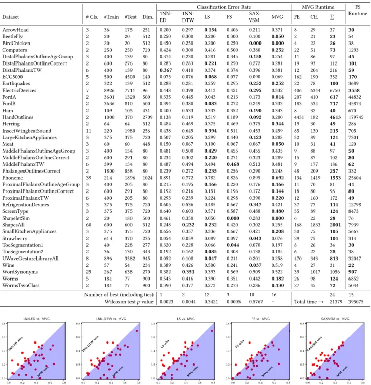
Viewing the error rate comparison columns in Table 3, it is
obvious that MVG is the most accurate classifier with 16
win-ning datasets. LS then follows MVG with 12 winwin-ning datasets. A
Wilcoxon test between MVG and LS yields ap-value of0.3421> 0.05, suggesting that MVG should not be considered significantly
better than LS. SAX-VSM is ranked third with 10 winning cases.
The Wilcoxon test again suggest that such difference is not
sta-tistically significant. However, MVG is indeed significantly more
accurate than FS, 1NN-DTW and 1NN-ED. Moreover, scatter
plots in Figure 8 shows that most of the points in each
compar-ison are located away from the diagonal line, suggesting that
MVG is indeed a very different approach when compared to the
state-of-the-art. Having confirmed MVG’s excellent accuracy, we
Table 3: Classification error rates compared with five benchmark approaches and running time statistics (in seconds).
Classification Error Rate MVG Runtime FS Runtime Dataset # Cls. #Train #Test Dim.
1NN-ED 1NN-DTW LS FS SAX-VSM MVG FE Clf. Í ArrowHead 3 36 175 251 0.200 0.297 0.154 0.406 0.211 0.371 8 29 37 30 BeetleFly 2 20 20 512 0.250 0.300 0.200 0.300 0.100 0.050 2 21 23 54 BirdChicken 2 20 20 512 0.450 0.250 0.200 0.250 0.000 0.000 4 22 26 38 Computers 2 250 250 720 0.424 0.300 0.416 0.500 0.380 0.252 22 51 73 1293 DistalPhalanxOutlineAgeGroup 3 400 139 80 0.374 0.230 0.281 0.345 0.158 0.254 11 86 97 45 DistalPhalanxOutlineCorrect 2 600 276 80 0.283 0.283 0.221 0.250 0.272 0.281 19 93 112 101 DistalPhalanxTW 6 400 139 80 0.367 0.410 0.374 0.374 0.396 0.381 12 204 216 59 ECG5000 5 500 4500 140 0.075 0.076 0.068 0.077 0.090 0.069 162 190 352 170 Earthquakes 2 322 139 512 0.288 0.281 0.259 0.295 0.252 0.252 22 78 100 3689 ElectricDevices 7 8926 7711 96 0.448 0.398 0.413 0.421 0.295 0.332 406 6344 6750 3558 FordA 2 3601 1320 500 0.335 0.445 0.043 0.213 0.173 0.014 207 410 617 44832 FordB 2 3636 810 500 0.394 0.380 0.083 0.272 0.249 0.333 183 534 717 45874 Ham 2 109 105 431 0.400 0.533 0.333 0.352 0.190 0.343 8 32 40 670 HandOutlines 2 1000 370 2709 0.138 0.119 0.519 0.189 0.092 0.200 4431 182 4613 179745 Herring 2 64 64 512 0.484 0.469 0.375 0.469 0.375 0.344 19 30 49 286 InsectWingbeatSound 11 220 1980 256 0.438 0.645 0.394 0.511 0.453 0.459 85 130 215 705 LargeKitchenAppliances 3 375 375 720 0.507 0.205 0.299 0.440 0.123 0.288 32 89 121 7301 Meat 3 60 60 448 0.150 0.067 0.100 0.067 0.067 0.050 10 31 41 120 MiddlePhalanxOutlineAgeGroup 3 400 154 80 0.481 0.500 0.429 0.455 0.455 0.435 9 88 97 50 MiddlePhalanxOutlineCorrect 2 600 291 80 0.234 0.302 0.220 0.271 0.323 0.289 15 87 102 80 MiddlePhalanxTW 6 399 154 80 0.487 0.494 0.494 0.468 0.513 0.481 9 177 186 62 PhalangesOutlinesCorrect 2 1800 858 80 0.239 0.272 0.235 0.256 0.290 0.248 48 209 257 332 Phoneme 39 214 1896 1024 0.891 0.772 0.782 0.826 0.895 0.692 134 1419 1553 25604 ProximalPhalanxOutlineAgeGroup 3 400 205 80 0.215 0.195 0.166 0.220 0.176 0.166 11 70 81 41 ProximalPhalanxOutlineCorrect 2 600 291 80 0.192 0.216 0.151 0.196 0.172 0.144 18 80 98 80 ProximalPhalanxTW 6 400 205 80 0.293 0.239 0.224 0.298 0.390 0.220 12 160 172 49 RefrigerationDevices 3 375 375 720 0.605 0.536 0.485 0.667 0.347 0.421 37 77 114 12798 ScreenType 3 375 375 720 0.640 0.603 0.571 0.587 0.488 0.480 35 89 124 8473 ShapeletSim 2 20 180 500 0.461 0.350 0.050 0.000 0.283 0.000 6 22 28 76 ShapesAll 60 600 600 512 0.248 0.232 0.232 0.420 0.302 0.255 168 1833 2001 7939 SmallKitchenAppliances 3 375 375 720 0.656 0.357 0.336 0.667 0.421 0.208 30 75 105 5667 Strawberry 2 613 370 235 0.054 0.059 0.089 0.097 0.043 0.076 29 75 104 314 ToeSegmentation1 2 40 228 277 0.320 0.228 0.066 0.044 0.070 0.197 8 26 34 30 ToeSegmentation2 2 36 130 343 0.192 0.162 0.085 0.308 0.138 0.185 6 22 28 38 UWaveGestureLibraryAll 8 896 3582 945 0.052 0.108 0.047 0.211 0.201 0.258 470 343 813 32047 Wine 2 57 54 234 0.389 0.426 0.500 0.241 0.037 0.519 4 27 31 22 WordSynonyms 25 267 638 270 0.382 0.351 0.393 0.569 0.509 0.522 39 1017 1056 907 Worms 5 181 77 900 0.545 0.416 0.390 0.351 0.442 0.182 26 98 124 6852 WormsTwoClass 2 181 77 900 0.390 0.377 0.273 0.273 0.286 0.130 27 45 72 5044 Number of best (including ties) 1 2 12 3 10 16 24 15
Wilcoxon testp-value 0.0023 0.0044 0.3421 0.0005 0.5767 – Total time→ 21379 395075
0.0 0.2 0.4 0.6 0.8 0.0 0.2 0.4 0.6 0.8 1NN-ED wins MV Gwins 1NN-ED vs. MVG 0.0 0.2 0.4 0.6 0.8 0.0 0.2 0.4 0.6 0.8 1NN-DTW wins MV Gwins 1NN-DTW vs. MVG 0.0 0.2 0.4 0.6 0.8 0.0 0.2 0.4 0.6 0.8 LS wins MV Gwins LS vs. MVG 0.0 0.2 0.4 0.6 0.8 0.0 0.2 0.4 0.6 0.8 FS wins MV Gwins FS vs. MVG 0.0 0.2 0.4 0.6 0.8 0.0 0.2 0.4 0.6 0.8 SAXVSM wins MV Gwins SAXVSM vs. MVG
Figure 8: Comparison of classification accuracy with five state-of-the-art approaches in the form of scatter plots.
4.5
Efficiency
The pipeline of MVG consists of a feature extraction phase and a
train-validate-test process. During the feature extraction process,
time series are firstly transformed in to VGs and then features are
extracted from such graphs. With optimization from [1],
trans-forming time series of lengthn into VGs has a computation complexity ofO(nlog2(n))and it can be effectively solved within
O(log2(n))time when taking full advantage of parallelization. Extracting motif features from VGs may be potentially
expen-sive, fortunately PGD provides a fully parallel way of counting
small motifs. For instance, counting graph cliques of size 4 – one
of the most time consuming tasks in PGD – has a computation
complexity ofO(m·∆·Tmax), wheremis the number of 4-motifs
(i.e., 11),∆is the maximum degree andTmax is the maximum number of triangles incident to an edge andTmax≪∆. PGD is hundreds of times faster than other motif counting algorithms:
counting motifs from a graph with more than 26,000 vertices
can take only 0.01 seconds on a twelve-core commodity CP U [2].
Since other statistic features such as density,k-core, assortativity and degree statistics extracted from time series VGs are
inten-tionally chosen to be simple metrics, collecting these features has
a time complexity ofO(max(|V|,|E|)). Since we use a multiscale graph representation, ultimately graph generation has a
mono-thread complexity ofO(nlog3(n))and in parallel anO(log3(n)) time complexity. As a result, feature extraction per graph has a
classification process leverages state-of-the-art classifiers that are
widely used and well-optimized. Overall, the efficiency of MVG
may be best illustrated when we compare our method against
our benchmarking approaches.
Previous research [42] has shown that LS is extremely time
consuming, and FS as an approximated approach can be 100X
faster than LS. As a result, FS will be a good and strong baseline
to which the running time of our approach can be compared.
Thus we record the running time of FS and MVG and compare
their efficiency. These experiments are conducted on a computer
with Intel i7-4980HQ quad-core CP U clocked at 2.80GHz, 16GB
memory and solid-state drive suitable for fast I/O. We use the
FS implementation by its original authors [35] with default
pa-rameters. Columns located on the right side of Table 3 shows
the running time per dataset for MVG and FS. For MVG, running
time for feature extraction and training are recorded separately
and then summed. Overall, MVG completes faster than FS for 24
datasets. The total running time of FS for all 39 datasets amounts
to 395075 seconds, which is more than 18 times that of MVG.
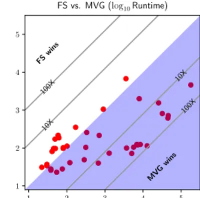
A scatter plot of the running time is provided in Figure 9,
obvi-ously MVG can be up to 100X faster than FS, suggesting that it
is indeed an efficient TSC approach. In addition, we note that
FS appears to be time consuming with large datasets with time
series of high dimensionality, while the running time of MVG
remains reasonable as datasets grow larger. Furthermore, since
we have experimented only on a quad-core commodity computer
that is not really powerful in terms of parallel processing, the
efficiency of MVG can be easily boosted by adding more
comput-ing cores. Overall, MVG can indeed be considered an efficient
TSC approach. 1 2 3 4 5 1 2 3 4 5 FS wins MV Gwins 100X 10X 10X 100X FS vs. MVG (log10Runtime)
Figure 9: Runtime comparison between FS and MVG.
4.6
Case Study
Although accuracy and efficiency are very important
measure-ments for TSC approaches, it is also desirable for TSC methods
to have comprehensible classification processes, so that users
may gain extra insights into his/her time series data. Popular
approaches based on shapelets and subsequences may have a
natural advantage in classification comprehensibility. However,
since features extracted in MVG are solely statistical, it can be
difficult to locate exactly where a distinguishing subsequence lies
in the original time series. However, for MVG it is still possible
to understand which features have contributed most to correct
classification. For instance, when feeding features to train an
XGBoost classifier, it will assign weights to all the features.
Af-ter ranking these features, we can also gain insights into the
data. For instance, Figure 10 illustrates a scatter matrix plot for
the test dataset ofFordAshowing ten most important features
learned by the classifier2. Out of ten features, six are features from HVGs, which are created from the original series (T0). VGs
features from dimensionality-reduced approximations (T2and T3) are also present. Moreover, it appears that most highly ranked
graph features for this dataset are MPDs and assortativity,
sug-gesting that statistics other than MPDs are indeed helpful. Finally,
visually from the kernel density estimation it is obvious that some
features alone –e.g.,T0HVGP(M44)– can already provide good classification guidelines, suggesting that it is feasible for MVG to
present visually comprehensible cues regarding its classification
decisions.
4.7
Discussions
Due to specific characteristics of VGs, obviously MVG may not be
suitable for every TSC scenarios. For instance, VGs are agnostic
of affine transformations in time series. That is, in applications
where the absolute oscillation is more important, MVG is less
likely to detect such characteristics. Furthermore, when dealing
with non-stationary time series data where trends are very
fre-quently found, MVG works best when trends are not the deciding
factor since VGs may not be able to capture long-term monolithic
trends. Since many graph features have been taken into account
in MVG, we believe it can be robust in practical applications.
In addition to limitations inherited from VGs, our approach is
more suitable for applications where the size of training datasets
is larger, so that classification models can generalize better. In
fact, when we review the classification accuracy of MVG, it seems
that a majority of its winning datasets have either long time series
or large training datasets. This is perhaps innate to the nature of
statistics: sample size has to be sufficiently large to make accurate
estimations. Based on running time comparison, MVG also scales
well with large datasets, which can be an important advantage
in the era of big data.
5
RELATED WORK
TSC is a major task in time series mining thanks to its wide
application scenarios. As a consequence, there are a plethora
of classification algorithms for TSC. Classical TSC approaches
involve utilizing 1NN classification together with similarity
mea-sures specific to time series data,e.g., DTW [7] and its variants with lower bounding [36] and early abandoning techniques [34].
Another line of research transforms time series into texts and
resort to text classification algorithms. For example, inspired by
the well knownbag-of-wordsapproach, [31] proposes the Bag-of-Patterns approach for TSC. SAX-VSM [39] also takes advantage
of bag-of-words approach and builds term frequency-inverse
document frequency (TF-IDF) vectors in its training phase. It defines a similarity measure of two vectors (that are constructed
from original series) based on their inner product. Both
Bag-of-Patterns and SAX-VSM rely on SAX [30] for transforming time
series into texts. A more recent work, Representative Pattern
Mining (RPM) [42], also tries to classify time series by means of
finding the most representative SAX-symbolized subsequences.
Our previous work Domain Series Corpus (DSCo) [24, 29] also
transforms time series into texts and approximates TSC to a
pseudo language detection problem. [38] invents another
sym-bolic representation based on Fourier transform and proposes a
bag-of-patterns approach named BOSS ensemble based on this
symbolic representation method.
2
To save space, we show more illustrations comparing original time series and important MVG features on project website. URL: http://daoyuan.li/mvg/
0.2 0.21 0.22 0.23 T0 HV G P ( M 31 ) 0.77 0.78 0.79 0.80 T0 HV G P ( M 32 ) 0.000080 0.000085 0.000090 T0 HV G P ( M 410 ) 0.26 0.27 0.28 T0 HV G P ( M 43 ) 0.000 0.001 0.002 0.003 T0 HV G P ( M 44 ) 0.50 0.55 0.60 T0 HV G P ( M 46 ) 0.0 0.2 0.4 T2 V G Asso rt. 0.50 0.55 0.60 T2 HV G P ( M 46 ) 0.0 0.2 0.4 T2 HV G Asso rt. 0 . 20 0 . 22 T0HVGP(M31) −0.1 0.0 0.1 0.2 T3 V G Asso rt. 0 . 78 0 . 80 T0HVGP(M32) 0.00008 0.00009 T0HVGP(M410) 0 . 26 0 . 28 T0HVGP(M43) 0 . 000 0 . 002 T0HVGP(M44) 0 . 5 0 . 6 T0HVGP(M46) 0 . 00 0 . 25 T2VG Assort. 0 . 5 0 . 6 T2HVGP(M46) 0 . 00 0 . 25 T2HVG Assort. 0 . 0 0 . 2 T3VG Assort.
Figure 10: Scatter matrix of ten most important features for FordA’s test dataset. Different point colors indicate different classes and the diagonal shows the Gaussian kernel density estimation for each feature.
Recently, shapelet-based approaches are gaining popularity
among the research community. A shapelet [47] is a single
subse-quence in time series that is representative of its class. However,
these approaches [15, 16] are known for their high computation
complexity. As we have demonstrated in this paper, FS [35] as
an approximated approach can also take long time to run. High
computation complexity is also present for TSC approaches using
deep neural networks [46]. Finally, [4] introduce an ensemble
algorithm named Collective of Transformation-based Ensembles
(COTE) – an ensemble of 35 different classifiers – that has shown
to be very accurate but has a time complexity ofO(m4n2), where
mis the dimensionality of time series andnis the size of training dataset.
Although the concept of time series VGs has appeared for
almost a decade, using it for TSC has just started picking up.
Machine learning approaches taking advantage of VG and its
variants are generally using artificially generated data [45] or
EEG signals. Finally, graph kernel methods [20] can be used
for evaluating graph similarity, which may potentially be used
for TSC as well. Our approach transforms TSC into a graph
classification [14] problem. Since we convert time series into
a set of graphs at different scales, we have not experimented
generic graph classification algorithms. However, they are indeed
interesting for future experiments.
6
CONCLUSIONS AND FUTURE WORK
This paper proposes a graph-based multiscale time series
rep-resentation named MVG and a feature extraction method for
TSC. MVG transforms time series into a collection of visibility
graphs of various scales and feature extraction are conducted by
investigating statistical graph features such as probability