Fast boosting using adversarial bandits
R. Busa-Fekete, B. K´
egl
To cite this version:
R. Busa-Fekete, B. K´
egl. Fast boosting using adversarial bandits. J. F¨
urnkranz, T. Joachims.
27th International Conference on Machine Learning (ICML 2010), Jun 2010, Haifa, Israel.
pp.143-150, 2010.
<in2p3-00614564>
HAL Id: in2p3-00614564
http://hal.in2p3.fr/in2p3-00614564
Submitted on 12 Aug 2011
HAL
is a multi-disciplinary open access
archive for the deposit and dissemination of
sci-entific research documents, whether they are
pub-lished or not.
The documents may come from
teaching and research institutions in France or
abroad, or from public or private research centers.
L’archive ouverte pluridisciplinaire
HAL
, est
destin´
ee au d´
epˆ
ot et `
a la diffusion de documents
scientifiques de niveau recherche, publi´
es ou non,
´
emanant des ´
etablissements d’enseignement et de
recherche fran¸
cais ou ´
etrangers, des laboratoires
publics ou priv´
es.
Fast boosting using adversarial bandits
R´obert Busa-Fekete1,2 [email protected]
Bal´azs K´egl1 [email protected]
1LAL/LRI, University of Paris-Sud, CNRS, 91898 Orsay, France
2Research Group on Artificial Intelligence of the Hungarian Academy of Sciences and University of Szeged, Aradi
v´ertan´uk tere 1., H-6720 Szeged, Hungary
Abstract
In this paper we apply multi-armed ban-dits (MABs) to improve the computational complexity of AdaBoost. AdaBoost con-structs a strong classifier in a stepwise fashion by selecting simple base classifiers and us-ing their weighted “vote” to determine the final classification. We model this stepwise base classifier selection as a sequential de-cision problem, and optimize it with MABs where each arm represents a subset of the base classifier set. The MAB gradually learns the “usefulness” of the subsets, and selects one of the subsets in each iteration. Ad-aBoost then searches only this subset in-stead of optimizing the base classifier over the whole space. The main improvement of this paper over a previous approach is that we use an adversarial bandit algorithm instead of stochastic bandits. This choice allows us to prove a weak-to-strong-learning theorem, which means that the proposed technique re-mains a boosting algorithm in a formal sense. We demonstrate on benchmark datasets that our technique can achieve a generalization performance similar to standardAdaBoost
for a computational cost that is an order of magnitude smaller.
1. Introduction
AdaBoost (Freund & Schapire, 1997) is one of the best off-the-shelf learning methods developed in the last decade. It constructs a classifier in a stepwise fashion by adding simple classifiers (called base
clas-Appearing inProceedings of the 27thInternational Confer-ence on Machine Learning, Haifa, Israel, 2010. Copyright 2010 by the author(s)/owner(s).
sifiers) to a pool, and using their weighted “vote” to determine the final classification. The simplest base learner used in practice is thedecision stump, a one-decision two-leaf one-decision tree. Learning a one-decision stump means selecting a feature and a threshold, so the running time ofAdaBoostwith stumps is propor-tional to the number of data points n, the number of attributesd, and the number of boosting iterationsT. Whentrees(Quinlan,1993) orproducts(K´egl & Busa-Fekete, 2009) are constructed over the set of stumps, the computational cost is multiplied by an additional factor of the number of tree levels logN (where N
is the number of leaves) or the number of terms m. Although the running time is linear in each of these factors, the algorithm can be prohibitively slow if the data size nand/or the number of features dis large. There are essentially two ways to accelerate
AdaBoost in this setting: one can either limit the number of data pointsnused to train the base learn-ers, or one can cut the search space by using only a subset of the d features. Although both approaches increase the number of iterationsT needed for conver-gence, the net computational time can still be signifi-cantly decreased. The former approach has a basic ver-sion when the base learner is not trained on the whole weighted sample, rather on a small subset selected ran-domly using the weights as a discrete probability dis-tribution (Freund & Schapire, 1997). A recently pro-posed algorithm of this kind isFilterBoost(Bradley & Schapire, 2008), which assumes that an oracle can produce an unlimited number of labeled examples, one at a time. In each boosting iteration, the oracle gen-erates sample points that the base learner can either accept or reject, and then the base learner is trained on a small set of accepted points. The latter approach was proposed by (Escudero et al.,2000) which introduces several feature selection and ranking methods used to accelerate AdaBoost. In particular, the Lazy-Boost algorithm chooses a fixed-size random subset
of the features in each boosting iteration, and trains the base learner using only this subset. This technique was successfully applied to face recognition where the number of features can be extremely large (Viola & Jones,2004).
Recently, (Busa-Fekete & K´egl,2009) proposed an im-provement of LazyBoost by replacing the random selection by a biased selection towards features that proved to be useful in previous iterations. Learn-ing the usefulness was achieved by usLearn-ing multi-armed bandit (MAB) algorithms. They used a stochastic MAB (UCB(Auer et al.,2002a)) which assumes that the rewards are generated randomly from a station-ary distribution. The algorithm was successful in ac-celerating AdaBoostin practice, but due to the in-herently non-stochastic nature of the rewards, (Busa-Fekete & K´egl,2009) could not state anything on the algorithmic convergence of the technique, and so the connection betweenAdaBoostand bandits remained slightly heuristic.
In this paper we propose to useadversarialbandits in-stead of stochastic bandits in a similar setup. In this model the rewards are not assumed to be drawn from a stationary distribution, and they can depend arbi-trarily on the past. Using adversarial bandits, we can prove a weak-to-strong-learning theorem which means that the proposed technique remains a boosting rithm in a formal sense. Furthermore, the new algo-rithm also appears good in practice: if anything, it seems better in terms of generalization performance, and, above all, in computational complexity.
The paper is organized as follows. We start by re-viewing the technical details of the AdaBoost.MH
algorithm and the base learners we will use in the ex-periments in Section 2. Section 3 contains our main results where we describe the adversarial MAB algo-rithm and its interaction with AdaBoost.MH, and state our weak-to-strong learning result for the pro-posed algorithm. We present our experimental results in Section 4 where first we demonstrate on synthetic data sets that the bandit based algorithms are indeed able to discover useful features, then we furnish re-sults on benchmark data sets that which indicate that the proposed algorithm improves the running time of
AdaBoost.MH by at least an order of magnitude, without losing much of its generalization capacity.
2. AdaBoost.MH
For the formal description, letX= (x1, . . . ,xn) be the n×dobservation matrix, where x(j)i are the elements of thed-dimensional observation vectorsxi∈Rd. We
are also given a label matrix Y = (y1, . . . ,yn) of
di-mensionn×K whereyi∈ {+1,−1}K. Inmulti-class
classification one and only one of the elements of yi
is +1, whereas in multi-label (or multi-task) classifi-cation yi is arbitrary, meaning that the observation
xi can belong to several classes at the same time. In
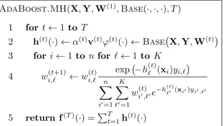
the former case we will denote the index of the correct class by!(xi). AdaBoost.MH(X,Y,W(1),Base( ·,·,·), T) 1 fort←1to T 2 h(t)( ·)←α(t)v(t)ϕ(t)( ·)←Base!X,Y,W(t)" 3 for i←1to nfor !←1to K
4 wi,!(t+1)←wi,!(t) exp ! −h(t)! (xi)yi,!" n # i!=1 K # !!=1 wi(t)!,!!e−h (t) !!(xi!)yi!,!! 5 return f(T)( ·) =$Tt=1h(t)( ·)
Figure 1.The pseudocode of the AdaBoost.MH
algo-rithm. X is the observation matrix, Y is the label ma-trix, W(1) is the initial weight matrix, Base(·,·,·) is the base learner algorithm, andT is the number of iterations.
α(t)is the base coefficient,v(t)is the vote vector,ϕ(t)(·) is the scalar base classifier, h(t)(
·) is the vector-valued base classifier, andf(T)(
·) is the final (strong) classifier.
The goal of theAdaBoost.MHalgorithm ( (Schapire & Singer,1999), Figure1) is to return a vector-valued classifierf :X →RK with a smallHamming loss
RH!f(T),W(1)"= n # i=1 K # !=1
wi,!(1)I%sign!f!(T)(xi)"&=yi,! &
1
by minimizing its upper bound (the exponential mar-gin loss) Re!f(T),W(1)"= n # i=1 K # !=1
wi,!(1)exp!−f!(T)(xi)yi,!",
(1) where f!(xi) is the !th element of f(xi). The
user-defined weights W(1) = 'w(1) i,! (
are usually set either uniformly towi,!(1) = 1/(nK), or, in the case of multi-class multi-classification, to
w(1)i,! =
) 1
2n if!=!(xi) (i.e., ifyi,!= 1), 1
2n(K−1) otherwise (i.e., ifyi,!=−1)
(2)
to createKwell-balanced one-against-all classification problems. AdaBoost.MHbuilds the final classifierf as a sum of base classifiers h(t) :
X → RK returned
iterationt. In general, the base learner should seek to minimize thebase objective
E!h,W(t)"= n # i=1 K # !=1
w(t)i,!exp!−h!(xi)yi,! "
. (3)
Using the weight update formula of Line4(Figure1), it can be shown that
Re!f(T),W(1)"= T * t=1
E!h(t),W(t)", (4) so minimizing (3) in each iteration is equivalent to min-imizing (1) in an iterative greedy fashion. By obtain-ing the multi-class prediction!+(x) = arg max!f
(T) ! (x),
it can also be proven that the “traditional” multi-class loss (orone-error)
R!f(T)"= n # i=1 I%!(xi)&=!+(xi) & (5)
has an upper bound KRe!f(T),W(1)" if the weights
are initialized uniformly, and √K−1Re!f(T),W(1)"
with the multi-class initialization (2). This justifies the minimization of (1).
2.1. Learning the base classifier
In this paper we usediscreteAdaBoost.MHin which the vector-valued base classifierh(x) is represented as
h(x) =αvϕ(x), (6)
whereα∈R+is thebase coefficient,v
∈ {+1,−1}Kis
thevote vector, andϕ(x) :Rd→ {+1,−1} is ascalar
base classifier. It can be shown that to minimize (3), one has to choose avand aϕthat maximize theedge
γ= n # i=1 K # !=1 wi,!v!ϕ(xi)yi,!. (7)
The optimal coefficient is then
α= 1
2log 1 +γ
1−γ.
It is also well known that the base objective (3) can be expressed as
E!h,W"=,(1 +γ)(1−γ) =,1−γ2. (8)
The simplest scalar base learner used in practice is the decision stump, a one-decision two-leaf decision tree of the form ϕj,b(x) = ) 1 ifx(j) ≥b, −1 otherwise, (9)
wherejis the index of the selected feature andbis the decision threshold.
Although boosting decision stumps often yields sat-isfactory results, the state-of-the-art performance of
AdaBoostis usually achieved by usingdecision trees as base learners, parametrized by their number of leaves N. We also test our approach using a re-cently proposed base learner that seems to outper-form boosted trees on large benchmarks (K´egl & Busa-Fekete, 2009). The goal of this learner is to optimize products of simple base learners of the form h(·) =
α-mj=1vjϕj(·), where the vote vectorsvj are
multi-plied element-wise. The base learner is parametrized by the number of termsm.
3. Reducing the search space of the
base learners using multi-armed
bandits
This section contains our main results. In Section3.1 we provide some details on MAB algorithms neces-sary for understanding our approach. Section 3.2 de-scribes the concrete MAB algorithm Exp3.Pand its interaction with AdaBoost.MH. Section 3.3 gives our weak-to-strong learning result for the proposed algorithm AdaBoost.MH.Exp3.P. Finally, in Sec-tion3.4 we elaborate some of the algorithmic aspects of the generic technique.
3.1. The multi-armed bandit problem
In the classical stochastic bandit problem the deci-sion maker pulls an arm out of M arms at discrete time steps. Selecting an arm j(t) in iteration t
re-sults in a random reward rj(t)(t) ∈ [0,1] coming from
a stationary distribution. The goal of the decision maker is to maximize the expected sum of the re-wards received. Intuitively, the decision maker has to strike a balance between using arms with large past rewards (exploitation) and trying arms that have not been tested enough times (exploration). Formally, let
G(T) =$T t=1r
(t)
j(t) be the total reward that the
deci-sion maker receives up to theTth iteration. Then the performance of the decision maker can be evaluated in terms of the regret with respect to the best arm ret-rospectively, defined asTmax1≤j≤Mµj−G(T) where µj is the (unknown) expected reward of thejth arm.
Contrary to the classical stochastic MABs, in the ad-versarial setup (Auer et al., 1995) there is a sec-ond, non-random player that chooses a reward vector r(t) ∈ RM in each iteration. There is no restriction
on the series of reward vectorsr(t), in particular, they
ac-tions. Only the rewardrj(t)(t) of the chosen arm j(t) is
revealed to the decision maker. Since the rewards are not drawn from a stationary distribution, any kind of regret can only be defined with respect to a particular sequence of actions. The most common performance measure is theweak regret
max j T # t=1 rj(t)−GT (10)
where the decision maker is compared to the best fixed arm retrospectively. We will denote this arm byj∗ = arg maxj
$T t=1r
(t)
j and its regret byG∗.
3.2. Accelerating AdaBoost using multi-armed bandits
The general idea is to partition the base classifier space H into (not necessarily disjunct) subsets G =
.
H1, . . . ,HM/and use MABs to learn the usefulness
of the subsets. Each arm represents a subset, so, in each iteration, the bandit algorithm selects a subset. The base learner then finds the best base classifier in the subset (instead of searching through the whole space H), and returns a reward based on this optimal base learner.
The upper bound (4) along with (8) suggest the use ofrj(t)=−log
0
1−γH(t)j2 as a reward function where
γH(t)j is the edge (7) of the classifier chosen by the base learner from Hj in thtth iteration. Since γ ∈ [0,1],
this reward is unbounded. To overcome this technical problem, we capr(t)j by 1 and define the reward as
r(t)j = min 1 1,−log 0 1−γH(t)j2 2 . (11)
This is equivalent of capping the edge γH(t)j at γmax =
0.93 which is rarely exceeded in practice, so this con-straint does not affect the practical performance of the algorithm.
(Busa-Fekete & K´egl, 2009) used this setup recently in the stochastic settings (with a slightly different re-ward). There are many applications where stochas-tic bandits have been applied successfully in a non-stationary environment, e.g., in a performance tun-ing problem (De Mesmay et al., 2009) or in the SAT problem (Maturana et al., 2009). The UCB (Auer et al., 2002a) and theUCBV (Audibert et al.,2009) algorithms work well in practice for accelerating Ad-aBoost, but the mismatch between the inherently ad-versarial nature of AdaBoost(the edgesγj(t) are
de-terministic) and the stochastic setup of UCB made it
impossible to derive weak-to-strong-learning-type per-formance guarantees onAdaBoost, and so in (Busa-Fekete & K´egl, 2009) the connection between Ad-aBoostand bandits remained slightly heuristic. In this paper we propose to use an adversarial MAB algorithm that belongs to the class of Exponentially Weighted Average Forecaster (EWAF) methods (Cesa-Bianchi & Lugosi,2006). In general, an EWAF algo-rithm maintains a probability distributionp(t)over the
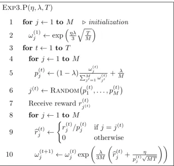
arms and draws a random arm from this distribution in each iteration. The probability value of an arm in-creases exponentially with the average of past rewards. In particular, we chose the Exp3.P algorithm (Auer et al., 2002b) (Figure2) because the particular form of the high-probability bound on the weak regret al-lows us to derive a weak-to-strong-learning result for
AdaBoost.MH. We call the combined algorithm Ad-aBoost.MH.Exp3.P. Exp3.P(η, λ, T) 1 forj←1 to M ' initialization 2 ωj(1)←exp3ηλ3 4T M 5 3 fort←1to T 4 for j←1to M 5 p(t)j ←(1−λ) ω (t) j !M j!=1ω (t) j! + λ M 6 j(t) ←Random!p(t)1 , . . . , p(t)M" 7 Receive rewardrj(t)(t) 8 for j←1to M 9 r+j(t)← ) rj(t)/p (t) j ifj =j(t) 0 otherwise 10 ω(t+1)j ←ω (t) j exp 6 λ 3M 6 + r(t)j +p(t)η j √ M T 77
Figure 2.The pseudocode of theExp3.Palgorithm. η >0
and 0 < λ ≤ 1 are “smoothing” parameters: the larger they are, the more uniform is the probability vector p(t),
and so the more the algorithm explores (vs. exploits). T
is the number of iterations. Exp3.P sends j(t) (Line 6) toAdaBoost.MH, and receives its reward in Line7from
AdaBoost.MH’s base learner via (11).
3.3. A weak-to-strong-learning result using Exp3.P with AdaBoost.MH
A sufficient condition for an algorithm to be called boosting is that, given a Base learner which always returns a classifier h(t) with edge γ(t) ≥ ρ for given ρ > 0, it returns a strong classifier f(T) with zero training error after a logarithmic number of iterations
satisfies this condition (Theorem 3 in (Schapire & Singer, 1999)). In the following theorem we prove a similar result forAdaBoost.MH.Exp3.P.
Theorem 1. LetHbe the class of base classifiers and
G=.H1, . . . ,HM/be an arbitrary partitioning of H.
Suppose that there exists a subsetHj† inG and a
con-stant 0 < ρ≤γmax such that for any weighting over
the training data setD, the base learner returns a base classifier fromHj† with an edgeγH
j† ≥ρ. Then, with
probability at least1−δ, the training errorR!f(T)"of
AdaBoost.MH.Exp3.Pwill become 0 after at most
T = max 1 log2M δ , 6 4C ρ2 74 ,4 log ! n√K−1" ρ2 2 (12)
iterations, whereC=√32M+√27MlogM+ 16,and the input parameters of AdaBoost.MH.Exp3.Pare set to λ= min 1 3 5,2 0 3 5 MlogM T 2 , η= 2 0 logM T δ . (13)
Proof. The proof is based on Theorem 6.3 of (Auer et al., 2002b) where the weak regret (10) of Exp3.P
is bounded from above by
4 0 M TlogM T δ + 4 0 5 3M TlogM+ 8 log M T δ
with probability 1−δ. Since this bound does not de-pend on the number of data points n, it is relatively easy to obtain the most important third term of (12) that ensures the logarithmic dependence of T on n. The technical details of the proof are included as sup-plementary material.
Remark 1 The fact that Theorem1 provides a large probability bound does not affect the PAC strong learning property of the algorithm since T is sub-polynomial in 1/δ (first term of (12)).
Remark 2 Our weak-learning condition is stronger than in the case of AdaBoost.MH: we require ρ -weak-learnability in the best subset Hj†, as opposed
to the whole base classifier set H. In a certain sense, a smaller ρ (and hence a larger number of iterations in principle) is the price we pay for doing less work in each iteration. The three terms of (12) comprise an in-teresting interplay between the number of subsetsM, the size of the subsets (in terms of the running time of the base learner), the quality of the subsets (in terms ofρ), and the number of iterationsT. In principle, it should be possible to optimize these parameters so as to minimize the total running time of the algorithm (to
achieve zero training error) in a similar framework to what was proposed by (Bottou & Bousquet,2008). In practice, however such an optimization is limited since, on the one hand, the quality of the subsets is unknown beforehand, and on the other, the bound (12) is quite loose in an absolute sense.
Remark 3 Applying Theorem 6.3 of (Auer et al., 2002b) requires that we formally set λ and η to the values in (13). However, it is a general practice to val-idate these parameters. In our experiments we found that both of them should be set to relatively small values (λ ≈ 0.15, η ≈ 0.3), which accords with the suggestions of (Kocsis & Szepesv´ari,2005).
3.4. Partitioning the base classifier set
In the case of simple decision stumps (9) the most nat-ural partitioning is to assign a subset to each feature:
Hj = .ϕj,b(x) : b ∈ R/. All our experiments were
carried out using this setup. One could think about making a coarser partitioning (more then one feature per subset), however, it makes no sense to split the features further since the computational time of find-ing the best threshold b on a feature is the same as that for evaluating a given stump on the data set. The situation is more complicated in the case of trees or products. In principle, one could set up a non-disjoint partitioning where every subset of N or m
features is assigned to an arm. This would make M
very big (dN or dm). Theorem 1 is still valid but in
practice the algorithm would spend all its time in the exploration phase, making it practically equivalent to
LazyBoost. To overcome this problem, we followed the setup proposed by (Busa-Fekete & K´egl, 2009) in which trees and products are modeled as sequences of decisions over the smaller partitioning used for stumps. The algorithm performs very well in practice using this setup. Finding a more accurate theoretical framework for this model is an interesting future task.
4. Experiments
4.1. Synthetic datasets
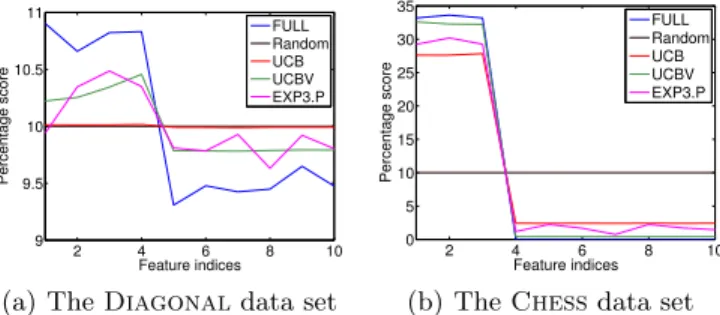
The goal of these experiments was to verify whether the bandit-based algorithms can indeed find useful fea-tures on data sets where the usefulness of the feafea-tures is entirely under our control. We used two baselines methods in each test: AdaBoost.MH with stumps (Full) andAdaBoost.MHthat searches only a ran-dom subset of base classifiers (Random), equivalent to
LazyBoost. We tested the methods on two binary classification tasks. In both tasksxare generated uni-formly in the d-dimensional unit cube, and only the first J features are relevant in determining the label.
In the first taskDiagonal(d, J, q), used by (Mease & Wyner,2007), the classes are separated by a diagonal cut on the first J features, and labels are perturbed by a small random noiseq. Formally,
P(Y = 1|x) =q+ (1−2q)I J # j=1 x(j)> J 2 .
In the second taskChess(d, J, L), the labels are gen-erated according to a chess board with L fields per dimension using the firstJ features. Formally,
y=
)
1 if $Jj=1+Lx(j)
,is pair
−1 otherwise
We run the algorithms on Diagonal(10,4,0.1) and
Chess(10,3,3) with n = 1000 data points. The parameters of AdaBoost.MH.Exp3.P were set to
T = 10000 and λ = η = 0.3. Figure 3 shows the percentage of the iterations when a certain feature was selected, averaged over 100 runs. The results are not very surprising: the bandit-based algorithms suc-ceeded in identifying the useful features most of the time, and chose them almost as frequently as full Ad-aBoost.MH. The only surprise was the performance of UCB on the Diagonaltask: it stuck in an explo-ration mode and failed to discover useful features.
2 4 6 8 10 9 9.5 10 10.5 11 Feature indices Percentage score FULL Random UCB UCBV EXP3.P
(a) TheDiagonaldata set
2 4 6 8 10 0 5 10 15 20 25 30 35 Feature indices Percentage score FULL Random UCB UCBV EXP3.P
(b) TheChessdata set
Figure 3.The percentage score of the iterations when a
certain feature was selected on (a) Diagonal(10,4,0.1) and (b)Chess(10,3,3) by the different algorithms.
4.2. Benchmark datasets
We tested the proposed method on five benchmark datasets using the standard train/test cuts2. We
com-pared AdaBoost.MH.Exp3.P (Exp3.P) with full
AdaBoost.MH (Full), AdaBoost.MH with ran-dom feature selection (Random), and two stochastic-bandit-based techniques of (Busa-Fekete & K´egl,2009)
2The data sets (selected based on their
wide usage and their large sizes) are
avail-able at yann.lecun.com/exdb/mnist (MNIST),
www.kernel-machines.org/data.html (USPS), and
www.ics.uci.edu/˜mlearn/MLRepository.html (letter,
pendigit, isolet).
(UCB and UCBV). In each run, we validated the number of iterations T using 80%-20% simple valida-tion. We smoothed the test error (5) on a window of
T /5 iterations to obtain R(T) = T5$6T /5t=4T /5R!f(t)",
and minimized R(T) in T. The advantage of this ap-proach is that this estimate is more robust in terms of random fluctuations than the raw errorR!f(T)". In
the case of trees and products, we also validated the hyperparametersN andmusing fullAdaBoost.MH, and used the validated values in all the algorithms. Fi-nally, for AdaBoost.MH.Exp3.Pwe also validated the hyperparametersλandηusing a grid search in the range of [0,0.6] with a resolution of 0.05.
Table 1 shows the test errors on the benchmark datasets. The first observation is that full Ad-aBoost.MH wins most of the time although the differences are rather small. The few cases where
Random or UCB/UCBV/Exp3.P beats full Ad-aBoost.MH could be explained by statistical fluc-tuations or the regularization effect of randomiza-tion. The second is thatExp3.Pseems slightly better than UCB/UCBV although the differences are even smaller.
Our main goal was not to beat full AdaBoost.MH
in test performance, but to improve its computational complexity. So we were not so much interested in the asymptotic test errors but rather the speed by which acceptable test errors are reached. As databases be-come larger, it is not unimaginable that certain algo-rithms cannot be run with their statistically optimal hyperparameters (T in our case) because of computa-tional limits, so managingunderfitting (an algorithmic problem) is more important than managing overfitting (a statistical problem) (Bottou & Bousquet, 2008). To illustrate how the algorithms behave in terms of computational complexity, we plotted the smoothed test error curves R(T) versustime for selected exper-iments in Figure 4. The improvement in terms of computational time over full AdaBoost.MH is of-ten close to an order of magnitude (or two in the case of MNIST), and Random is also significantly worse than the bandit-based techniques. The results also in-dicate thatExp3.Palso wins overUCB/UCBVmost of the time, and it is never significantly worse than the stochastic-bandit-based approach.
5. Discussion and Conclusions
In this paper we introduced a MAB based approach for accelerating AdaBoost. Using an adversarial setup, we were able to prove a high-probability weak-to-strong-learning bound, a result that was lacking from previous, more heuristic approaches using stochastic bandits. At the same time, in practice, the proposed
Table 1. Smoothed test error percentage scores (100R(T)) on benchmark datasets.
learner\data set MNIST USPS UCI pendigit UCI isolet UCI letter Stump/Full 7.56 6.28 4.96 4.52 14.57 Random 6.94 6.13 4.57 4.43 14.60 UCB 7.07 6.03 4.63 4.30 14.65 UCBV 7.02 6.08 4.63 4.43 14.77 EXP3.P 6.96 6.08 4.63 4.43 14.62 Product (m) 3 3 2 6 10 Full 1.26 4.37 1.89 3.86 2.31 Random 1.73 4.58 1.83 3.59 2.25 UCB 1.82 4.43 1.80 3.53 2.25 UCBV 1.85 4.53 1.92 3.53 2.20 EXP3.P 1.70 4.53 1.94 3.40 2.30 Tree (N) 17 15 19 8 38 Full 1.52 4.87 2.12 3.85 2.48 Random 1.82 5.13 2.06 3.78 3.08 UCB 2.30 4.98 2.09 3.85 3.10 UCBV 3.06 5.18 2.20 3.78 3.08 EXP3.P 1.85 4.93 2.06 3.72 3.02 104 106 0.075 0.08 0.085 0.09 0.095 0.1 Time in second MNIST/STUMP FULL Random UCB UCBV EXP3.P 102 103 104 0.04 0.05 0.06 0.07 0.08 0.09 0.1 Time in second USPS/TREE FULL Random UCB UCBV EXP3.P 101 102 103 104 0 0.02 0.04 0.06 0.08 0.1 Time in second PENDIGITS/PRODUCT FULL Random UCB UCBV EXP3.P 102 103 104 0.04 0.05 0.06 0.07 0.08 0.09 0.1 Time in second ISOLET/STUMP FULL Random UCB UCBV EXP3.P 103 104 105 0.02 0.03 0.04 0.05 0.06 0.07 0.08 0.09 0.1 Time in second LETTER/TREE FULL Random UCB UCBV EXP3.P 102 103 104 0.04 0.05 0.06 0.07 0.08 0.09 0.1 Time in second USPS/PRODUCT FULL Random UCB UCBV EXP3.P
Figure 4. Smoothed test errorsR(T) vs. total computational time.
algorithm performs at least as well as its stochastic counterpart in terms of both its generalization error and its computational efficiency. Although it seems that the asymptotic test error of AdaBoostwith full
search is hard to beat if we have enough computational resources, in large scale learning (recently described in a seminal paper by (Bottou & Bousquet, 2008)), where we stay in an underfitting regime so fast
op-timization becomes more important than asymptotic statistical optimality, our MAB-optimizedAdaBoost
has its place.
To keep the project within manageable limits, we con-sciously did not explore all the possible avenues in test-ing all possible on-line optimization algorithms. There are two particular ideas that we would like to inves-tigate in the near future. First, multi-armed bandits assume a stateless system, whereas AdaBoost has a natural state descriptor: the weight matrix W(t).
In this setup a Markov decision process would be more natural given that we can find a particular al-gorithm that can exploit a high dimensional, continu-ous state space and, at the same time, compete with bandits in computational complexity and convergence speed. The second avenue to explore is within the MAB framework: there are several successful appli-cations of AdaBoostwhere the number of features is huge but the feature space has an a-priori known structure (for example, Haar filters in image process-ing (Viola & Jones,2004) or word sequences in natural language processing (Escudero et al.,2000)). Classical bandits are hard to use in these cases but more recent MAB algorithms were developed for exactly this sce-nario (Coquelin & Munos,2007).
Acknowledgements
We would like to thank Peter Auer, Andr´as Gy¨orgy, and Csaba Szepesv´ari for their useful comments. This work was supported by the ANR-07-JCJC-0052 grant of the French National Research Agency.
References
Audibert, J.-Y., Munos, R., and Szepesv´ari, Cs. Exploration-exploitation tradeoff using variance es-timates in multi-armed bandits. Theor. Comput. Sci., 410(19):1876–1902, 2009.
Auer, P., Cesa-Bianchi, N., Freund, Y., and Schapire, R.E. Gambling in a rigged casino: The adversar-ial multi-armed bandit problem. In Proceedings of the 36th Ann. Symp. on Foundations of Computer Science, pp. 322–331, 1995.
Auer, P., Cesa-Bianchi, N., and Fischer, P. Finite-time analysis of the multiarmed bandit problem.Machine Learning, 47:235–256, 2002a.
Auer, P., Cesa-Bianchi, N., Freund, Y., and Schapire, R.E. The non-stochastic multi-armed bandit prob-lem. SIAM J. on Computing, 32(1):48–77, 2002b.
Bottou, L. and Bousquet, O. The tradeoffs of large
scale learning. In NIPS, volume 20, pp. 161–168, 2008.
Bradley, J.K. and Schapire, R.E. FilterBoost: Regres-sion and classification on large datasets. In NIPS, volume 20, 2008.
Busa-Fekete, R. and K´egl, B. Accelerating AdaBoost using UCB. InKDDCup 2009 (JMLR W&CP), vol-ume 7, pp. 111–122, 2009.
Cesa-Bianchi, N. and Lugosi, G. Prediction, Learning, and Games. Cambridge University Press, 2006. Coquelin, P-A. and Munos, R. Bandit algorithms for
tree search. InUAI, volume 23, 2007.
De Mesmay, F., Rimmel, A., Voronenko, Y., and P¨uschel, M. Bandit-based optimization on graphs with application to library performance tuning. In ICML, volume 26, pp. 729–736, 2009.
Escudero, G., M`arquez, L., and Rigau, G. Boosting applied to word sense disambiguation. In ECML, volume 11, pp. 129–141, 2000.
Freund, Y. and Schapire, R. E. A decision-theoretic generalization of on-line learning and an application to boosting. J. of Comp. and Sys. Sci., 55:119–139, 1997.
K´egl, B. and Busa-Fekete, R. Boosting products of base classifiers. In ICML, volume 26, pp. 497–504, 2009.
Kocsis, L. and Szepesv´ari, Cs. Reduced-Variance Pay-off Estimation in Adversarial Bandit Problems. In ECML Work. on Reinforcement Learning in Non-Stationary Environments, 2005.
Maturana, J., Fialho, ´A., Saubion, F., Schoenauer, M., and Sebag, M. Extreme compass and dynamic multi-armed bandits for adaptive operator selection. InIEEE ICEC, pp. 365–372, 2009.
Mease, D. and Wyner, A. Evidence contrary to the statistical view of boosting.JMLR, 9:131–156, 2007. Quinlan, J. C4.5: Programs for Machine Learning.
Morgan Kaufmann, 1993.
Schapire, R. E. and Singer, Y. Improved boosting al-gorithms using confidence-rated predictions. Mach. Learn., 37(3):297–336, 1999.
Viola, P. and Jones, M. Robust real-time face detec-tion. Int. J. of Comp. Vis., 57:137–154, 2004.