Radial Basis Functions: Biomedical Applications and Parallelization

(1)

University of Wisconsin Milwaukee

UWM Digital Commons

Theses and Dissertations

December 2016

Radial Basis Functions: Biomedical Applications

and Parallelization

Ke Liu

University of Wisconsin-Milwaukee

Follow this and additional works at:https://dc.uwm.edu/etd Part of theComputer Sciences Commons

This Dissertation is brought to you for free and open access by UWM Digital Commons. It has been accepted for inclusion in Theses and Dissertations by an authorized administrator of UWM Digital Commons. For more information, please [email protected].

Recommended Citation

Liu, Ke, "Radial Basis Functions: Biomedical Applications and Parallelization" (2016).Theses and Dissertations. 1382. https://dc.uwm.edu/etd/1382

(2)

RADIAL BASIS FUNCTIONS: BIOMEDICAL

APPLICATIONS AND PARALLELIZATION

by

Ke Liu

A Dissertation Submitted in

Partial Fulfilment of the

Requirements for the Degree of

Doctor of Philosophy

in Engineering

at

The University of Wisconsin-Milwaukee

(3)

ii

ABSTRACT

RADIAL BASIS FUNCTIONS: BIOMEDICAL APPLICATIONS AND

PARALLELIZATION

by

Ke Liu

The University of Wisconsin-Milwaukee, 2016

Under the Supervision of Professor Zeyun Yu

Radial basis function (RBF) is a real-valued function whose values depend only on the distances between an interpolation point and a set of user-specified points called centers. RBF

interpolation is one of the primary methods to reconstruct functions from multi-dimensional scattered data. Its abilities to generalize arbitrary space dimensions and to provide spectral accuracy have made it particularly popular in different application areas, including but not

limited to: finding numerical solutions of partial differential equations (PDEs), image processing, computer vision and graphics, deep learning and neural networks, etc.

The present thesis discusses three applications of RBF interpolation in biomedical engineering areas: (1) Calcium dynamics modeling, in which we numerically solve a set of PDEs by using meshless numerical methods and RBF-based interpolation techniques; (2) Image restoration and transformation, where an image is restored from its triangular mesh representation or

transformed under translation, rotation, and scaling, etc. from its original form; (3) Porous structure design, in which the RBF interpolation used to reconstruct a 3D volume containing

(4)

iii

porous structures from a set of regularly or randomly placed points inside a user-provided surface shape. All these three applications have been investigated and their effectiveness has been supported with numerous experimental results. In particular, we innovatively utilize anisotropic distance metrics to define the distance in RBF interpolation and apply them to the aforementioned second and third applications, which show significant improvement in

preserving image features or capturing connected porous structures over the isotropic distance-based RBF method.

Beside the algorithm designs and their applications in biomedical areas, we also explore several common parallelization techniques (including OpenMP and CUDA-based GPU programming) to accelerate the performance of the present algorithms. In particular, we analyze how parallel programming can help RBF interpolation to speed up the meshless PDE solver as well as image processing. While RBF has been widely used in various science and engineering fields, the current thesis is expected to trigger some more interest from computational scientists or students into this fast-growing area and specifically apply these techniques to biomedical problems such as the ones investigated in the present work.

(5)

iv

(6)

v

LIST OF FIGURES

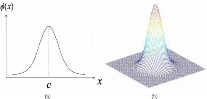
1.1 Figure 1 Gaussian basis function. (a) Shape of Gaussian basis function in 1D. c is the center. (b) Shape of Gaussian basis function in 2D...2

1.1 Figure 2 RBF support domains. (a) Compact support. (b) Non-compact support...3

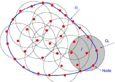
1.1 Figure 3 Discretization using meshless method: nodes, domains of influence (in circle shape). Blue line illustrates problem domain. Red dots illustrate nodes. Grey circle illustrates the influence of local domain Ω_𝐼.(Courtesy of [38])...4

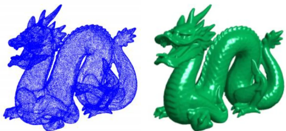
1.1 Figure 4 Surface reconstruction from point cloud. Left is the point cloud as input. Right is

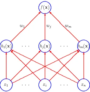
the reconstructed surface. (Courtesy of [45])...7 1.1 Figure 5 The traditional radial basis function network. 𝒙 = {𝑥_𝑖}_𝑖=1𝑛 is the input. 𝒉 =

{ℎ_𝑗} 𝑗=1 𝑚

are basis functions. The output 𝑓(𝒙)is the linear combination of weights 𝒘 = {𝑤_𝑗}

𝑗=1 𝑚

. (Courtesy of [46])...8

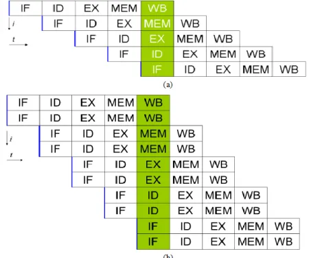
1.2 Figure 6 Illustration of instruction-level parallelism. (a) 5-stage pipeline RISC processor.

(b) 5-stage pipelined superscalar processor. (Courtesy of [58])...11

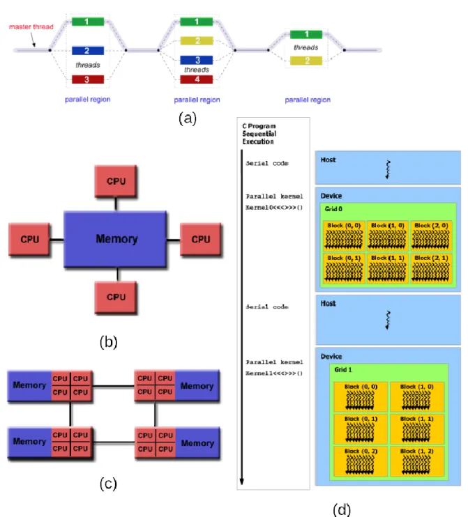
1.2 Figure 7 Different types of memory models of parallel computing. (a) Execution sequence

of shared memory model. Different colors illustrates different threads. (b) Shared memory model. (c) Distributed memory model. (d) Execution sequence of one of heterogeneous memory models. (Courtesy of [59] [60])...13

(10)

ix

2.2 Figure 8 (a) The model considered in current study, containing the t-tubule (blue), surrounding half sarcomere (red), and external cell membrane (green). (unit: 𝜇𝑚). (b) Flow chart of the meshless algorithm for modeling of calcium dynamics...22

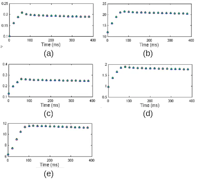
2.3 Figure 9 Results of calcium dynamics. Vertical coordinate illustrates concentrations in 𝜇𝑀.

(a) Concentration of Ca over time. (b) Concentration of Fluo over time. (c) Concentration of ATP over time. (d) Concentration of Cal over time. (e) Concentration of TN over time.24

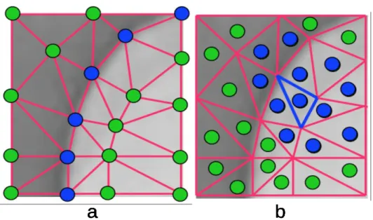
3.2 Figure 10 Example of interpolation. (a) Interpolation by vertices. Green dots are vertices

defined on feature. Blue dots are vertices defined on feature edge. (b) Interpolation by faces. Green dots are face centers. Blue dots are face centers used for interpolation of the intensities of pixels enclosed by the blue triangle...34 3.2 Figure 11 Interpolation schemes. (a) Isotropic RBF interpolation. (b) Anisotropic RBF interpolation. (c) Eigenvectors on an edge pixel. e1 shows the normal direction. e2 shows

the tangent direction...35 3.3 Figure 12 Resampling of original image (M × N) to target image (X × Y). As the gray triangle shows, every triangle in target image keeps the shape unchanged but has larger sampling density...41

3.4 Figure 13 Summary of restoration of Lena. (a) Original Lena image. (b) Result of piecewise

interpolation. (c) Result of vertex-based iso-RBF interpolation. (d) Result of triangle-based iso-RBF interpolation. (e) Result of triangle-based ARBF interpolation using MQ basis. (f) Result of triangle-based ARBF interpolation using IMQ basis...44

(11)

x

3.4 Figure 14 Details of Lena. (a) Original Lena image. (b) Generated mesh of (a). (c) Result

of triangle-based ARBF interpolation using MQ basis. (d) - (f) are zoomed-in views of (a) - (c), respectively...47 3.4 Figure 15 Details of brain MRI. (a) Original brain MRI. (b) Generated mesh of (a). (c) Result of triangle-based ARBF interpolation using MQ basis. (d) - (f) are zoomed-in views of (a) - (c), respectively...48

3.4 Figure 16 Details of breast MRI. (a) Original breast MRI. (b) Generated mesh of (a). (c)

Result of triangle-based ARBF interpolation using MQ basis. (d) - (f) are zoomed-in views of (a) - (c), respectively...49

3.4 Figure 17 Details of CT-scanned image of heart. (a) Original heart image. (b) Generated

mesh of (a). (c) Result of triangle-based ARBF interpolation using MQ basis. (d) - (f) are zoomed-in views of (a) - (c), respectively...50

3.4 Figure 18 Isotropic image translation and rotation. After transformation, image dimensions

are unchanged. (a) Image translated to another coordinates. Three red circles indicates image features before and after translation. (b) Left: original image. Right: image rotated

45°...51

3.4 Figure 19 Super-resolution results of biomedical images. Results are rescaled for display.

Red boxes show the zoom-in areas. (a) is the original brain MRI. (b) is the zoom-in part of (a). (c) is ARBF-5X SR result and (d) is bicubic-5X SR result. (e) is the original CT-scanned heart artery image. (f) is the zoom-in part of (e). (g) is ARBF-5X SR result. (h) is bicubic-5X SR result. (i) is the original breast MRI. (j) is zoom-in part of (i). (k) is ARBF-5X SR result. (l) is bicubic-ARBF-5X SR result...52

(12)

xi

4.3 Figure 20 Values assigned to mesh nodes. Red dots represent value of 1. Blue dots represent value of -1. In 3D meshes, interior dots are represented by lighter colors. (a) Sample 2D triangle mesh. Note both edge and triangle centers are given values -1. (b) Sample 3D tetrahedron mesh. Small triangle represent tetrahedron centers. (c) Sample 3D hexahedron mesh. Small triangle represent hexahedron centers...58

4.3 Figure 21 2D interpolation schemes. 𝑥 is the pixel to be interpolated. Dashed circle (for

RBF) or ellipses (for anisotropic RBF) are support domains of underlying basis functions. (a) RBF interpolation. (b) Anisotropic RBF interpolation………..59

4.3 Figure 22 Cases to calculate anisotropic distance. (a) Point x is on line segment (a,b). (b)

Point x and line segment (a,b) form an acute triangle then distance is deﬁned as the length of ‖𝑥𝑥′‖. (c) Point x and line segment (a,b) form an obtuse triangle. (d) Distance between line segment (a,b) and (c,d)...60

4.4 Figure 23 Results based on tetrahedron meshes. (a) Scaﬀold based on single tetrahedron.

(b) Input icosahedron mesh (formed by 20 tetrahedrons). (c) Scaﬀold using (b) as input...63

4.4 Figure 24 Results based on hexahedron meshes. (a) Scaﬀold based on single hexahedron.

(b) Scaﬀold based on 8 hexahedrons arranged to form a large cube. (c) Scaﬀold based on

4 hexahedrons arranged to form a rod shape...63 4.4 Figure 25 Results taken by diﬀerent values. (a) - (d) are results taken by increasing

iso-values...64

4.4 Figure 26 Results obtained by using different basis functions in ARBF interpolation. Shape

(13)

xii

Result interpolated by inverse multiquadrics (IMQ) basis. (c) Result interpolated by Gaussian basis. (d) Result interpolated by thin plate spline (TPS) basis...65

4.4 Figure 27 Experimental results. (a) Result interpolated by isotropic RBF and based on a

2D triangle mesh. (b-d) Results based on hexahedron meshes with disturbance...66

4.4 Figure 28 Porous structure obtained by TPMS method. (a) Structure obtained by P-type

function. (b) Structure obtained by D-type function. (c) Structure obtained by G-type function. (d) Structure obtained by IWP-type function...67 5.2 Figure 29 Column 1 shows the average concentrations of Ca2+, mobile and stationary buffers for point set 2 (30,807 points) in three implementations, namely, serial, OpenMP and CUDA. Note that the concentrations of the three versions are almost identical. Column 2 shows the average relative errors of point set 2 (30,807 points), as compared to the serial execution. Column 3 shows the average relative errors of point set 3 (234,921 points), as compared to the serial execution...75

(14)

xiii

LIST OF TABLES

3.3 Table 1 Summary of the Lena image (Figure 13)………46

3.3 Table 2 Summary of the three medical images (Figure 15, Figure 16, Figure 17)………...46

4.1 Table 3 Category of methods to design porous scaffolds in tissue engineering...54 4.3 Table 4 Type of distances used in porous structure construction...61

5.2 Table 5 Running time of Serial, OpenMP, CUDA implementations on 3 point sets (unit:

seconds)………..76

5.3 Table 6 Execution time of image restoration. Results are the almost identical for block size

(15)

xiv

ACKNOWLEDGEMENTS

First, I would sincerely express my gratitude to my advisor, Professor Zeyun Yu, to the continuous support and guide to my Ph.D. study and research, for his patience, motivation, and vast knowledge. His insightful thoughts and advice helped me a lot during the time of research and writing of this thesis.

Besides my advisor, I would very much like to thank all my thesis committee members: Professor Guangwu Xu, Professor Tian Zhao, Professor Lei Wang, and Professor Roshan D'Souza, for their valuable comments and encouragement.

My sincere thank also goes to Jason Bacon, who provided me access to the research cluster at UW-Milwaukee, and gave me instructions to use the cluster. Without his precious support, it would not be possible to conduct this research.

Last but not least, I would like to thank my family for their spiritual support throughout writing my PhD thesis and my life in general.

(16)

1

Chapter 1 Introduction

1.1 Radial Basis Function (RBF)

1.1.1 Definition

Radial Basis Function (RBF) is a real-valued function whose value depends only on the distance from two points in multi-dimensional space. One of these points is called the center, which could be the origin or alternatively some other point in this space. RBF interpolation is one of the primary methods to analyze multi-dimensional scattered data. Its abilities to generalize arbitrary space dimensions and to provide spectral accuracy have made it particular popular in different types of applications. Some of the applications include function approximation, numerical solutions of partial differential equations, computer vision and neural networks, etc.

RBF is formally defined as ϕ(𝑟) = ϕ(‖𝑟‖). Any function ϕ that satisfies the property ϕ(𝑟) = ϕ(‖𝑟‖) is a radial function. Norm usually is defined as the Euclidean norm but other distance

functions like taxicab metric or Łukaszyk–Karmowski metric are also used to define the norm in

some applications. Let r = ‖𝒙 − 𝒙_𝑖‖ (𝒙_𝑖 is center), c be a constant called shape parameter (or free parameter in some literatures), commonly used types of radial basis functions include

 Gaussian: ϕ(𝑟) = 𝑒−(𝑐𝑟)2

 Multiquadric (MQ): ϕ(𝑟) = √𝑟2 _{+ 𝑐}2

 Inverse multiquadric (IMQ): ϕ(𝑟) = 1

𝑟2_+𝑐2

 Thin plate spline (TPS): ϕ(𝑟) = 𝑟2ln (𝑟)

The shape parameter plays an important role for the accuracy but how to choose the value is still an open research topic. Most researchers choose the value by trial and error or some other ad hoc

(17)

2

means. Literatures [1] [2] [3] [4] [5] [6] [7]provides more details about choosing the value for shape parameter. Figure 1 shows the shape of Gaussian basis function. Every radial basis function has a support range, which is the footprint of the basis function. There are two types of support. Compact support or finite support: function value is zero outside of certain interval. Non-compact support or infinite support: there is no interval to limit the function values. Function value goes to infinite as the range goes to infinite. Figure 2 shows the two types of support domains.

RBFs are typically used to construct function approximations defined on scattered multi-dimensional data of the form

u(𝒙) = ∑ 𝑤_𝑖𝜙(‖𝒙 − 𝒙_𝑖‖) 𝑁

𝑖=1

( 1 )

where u(𝒙) is the approximated function that represented as a weighted sum of N radial basis functions. Each basis function is associated with a different center 𝒙_i and weight 𝑤_i. The weights

Figure 1 Gaussian basis function. (a) Shape of Gaussian basis function in 1D. c is the center. (b) Shape of Gaussian basis function in 2D.

(18)

3

can be determined by solving linear equations. Let u𝑖 = u(𝑥𝑖), by ( 1 ), the weights 𝑤i can be

solved by [ 𝜙₁₁ ⋯ 𝜙_1𝑁 ⋮ ⋱ ⋮ 𝜙_𝑁1 ⋯ 𝜙_𝑁𝑁 ] [ 𝑤₁ ⋮ 𝑤𝑁 ] = [ 𝑢1 ⋮ 𝑢𝑁 ] ( 2 )

where 𝜙_ji = 𝜙(𝒙_𝑗− 𝒙_𝑖). Once the unknown weights 𝑤_i are solved, function values can be evaluated by ( 1 ). Besides by solving the linear equations in ( 2 ), the unknown weights 𝑤i can

also be solved by other matrix methods like linear least squares.

This approximation scheme is particularly useful in time series prediction, control of nonlinear systems having sufficiently simple chaotic behavior, and 3D reconstruction in computer graphics.

1.1.2 Applications

1.1.2.1 Numeric Simulation

Recent development of computer technology has made it possible to simulate a number of complex natural phenomena in experiments. In these experiments, partial differential equations (PDEs) with initial and boundary conditions are important tools to describe many mathematical models. For

(19)

4

complex PDEs, analytic solutions are usually too complex, even impossible to obtain. Therefore, numerical solutions as an approximation of analytical solutions are instead the goal to obtain in practice. Many numerical methods have been developed to solve PDEs. Some classical methods that solve PDEs numerically based on polynomial interpolation are finite difference method (FDM), finite element method (FEM), finite volume method (FVM) and pseudo-spectral methods. These methods solve a set of linear equations which are constructed after the analysis of the entire problem domain is analyzed and divided into elements or meshes.

Although these polynomial based methods are very effective to solve certain types of PDEs in many fields, they have limitations too, mostly because of the mesh-based interpolation. Distorted or low quality meshes lead to higher errors and necessitate remeshing, which is a task consuming both time and human labor and often is not guaranteed to be feasible in timely manner in complex 3D geometries. Moreover, the underlying mesh-based structure makes them not well suited to solve problems with discontinuity boundaries. A way to deal with discontinuities is remeshing or discontinuous enrichment. Alternatively, the extended finite element method (XFEM) [8] [9] [10]

Figure 3 Discretization using meshless method: nodes, domains of influence (in circle shape). Blue line illustrates problem domain. Red dots illustrate nodes. Grey circle illustrates the influence of local domain Ω𝐼.(Courtesy of [38]).

(20)

5

[11] enriches the approximation space so that both strong and weak discontinuities can be captured. However, the involved difficulties of mesh-based interpolation are not only remeshing but also transiting problem states from old mesh to new mesh. Impact/penetration problem, explosion/fragmentation problem, flow pass obstacles problem, fluid-structure interaction problem and some biomedical simulations like the simulation and analysis of particular particles in cardiomyocytes during excitation and contraction are extremely difficult using the traditional methods introduced above.

RBF based methods, however, do not suffer from the adaptive remeshing procedures and the

approximation is built from nodes only. Thus they belong to a category of methods called meshless

methods or meshfree methods. Meshless methods are good at achieving exponential convergence rates on problems where traditional methods have difficulties or fail to solve. By constructing a univariate function with Euclidean norm, meshless methods turn a multi-dimensional problem into a one dimensional problem. One of the earliest meshless methods is the smooth particle hydrodynamics (SPH) method proposed by Lucy [12] and Gingold and Monaghan [13]. It was proposed to solve problems in astrophysics. Libersky et al. [14] were the first to apply SPH in solid mechanics. Other improved SPH methods are proposed as well [15] [16] [17] [18] [19]. In 1990s other weak form based methods were developed while SPH and their improved versions were based on strong form. One of the earliest meshless methods based on global weak form is the element-free Galerkin (EFG) method [20]. One year later, reproducing kernel particle method (RKPM) was developed in wavelets [21]. In contrast to EFG and RKPM methods which use intrinsic basis, other methods are developed to use extrinsic basis and the concept of partition of unity (PU). The extrinsic basis was used to increase the approximation order. Melenk and Babuska [22] proposed partition of unity finite element method (PUFEM) based on the similarity of

(21)

6

meshless method and FEM. This method is very similar to hp-cloud method which employs elements of variable size (h) and polynomial degree (p).

All meshless methods introduced above are based on global weak form of PDEs. Another type of meshless methods are based on local weak forms. The most popular method of this type is the meshless local Petrov-Galerkin (MLPG) method [23]. The main difference between MLPG and global weak form based methods such EFG and RKPM is that local weak form is generated on overlapping local subdomains, on which the integration is carried out. Another well-known method which is called moving point method is mainly applied in fluid mechanics [24] [25] [26]. Because there is no mesh, tool like k-dimensional tree (KD-Tree) is usually used to divide the space and find neighboring nodes during the construction of linear systems. As a result, instead of solving a large linear system, many smaller linear systems are solved. By solving problems in collocation fashion, which is more flexible than global methods, local RBF methods can construct more stable linear systems and are easier to implement. Literatures [1] [27] [23] [28] [29] [30] [31] [32] [33] [34] [35] [36] [37] [38] illustrate the efficacy and popularity of meshless methods in numerical areas. Giordano et al. proposes an RBF optimization method in hydrolysis area [39]. Figure 3 (courtesy of [38]) illustrates how meshless methods discretize problem domain. Red dots illustrate nodes whose values are used to approximate. Blue line illustrates problem boundary. Grey circle illustrates the influence of a subdomain.

1.1.2.2 Surface Reconstruction

RBFs find their usage in computer graphics fields as well such as surface or object reconstruction from point cloud, mesh repair, image registration, and field visualization in 2D or 3D, etc. Interpolating meshes with holes and reconstructing surfaces from point cloud are ubiquitous problems in computer graphics and computer aided design (CAD) areas. Because RBFs are

(22)

7

polyharmonic and fast to be fitted and evaluated, smooth surface or object can be reconstructed from point cloud in large amount (in millions). The smooth blending of surfaces ensures a manifold can be constructed and thus manufacturable, which is related to many problems in CAD. Smoothing and remeshing existing noisy surfaces are also important problems in both computer graphics and CAD. These problems are considered independent problems in most cases and receive much attentions [40]. RBFs have been used to reconstruct surfaces by Carr et al. [41], Savchenko [42], Turk and O’Brien [43] [44]. These works are limited to small problems by their

𝑂(𝑁2) storage and 𝑂(𝑁3) arithmetic operations. By reducing the number of RBF centers used, a fast fitting and evaluation method is proposed by Carr et al. [45]. Figure 4 (courtesy of [45]) illustrates the problem of surface reconstruction from point cloud.

1.1.2.3 Artificial Neural Networks

RBFs are very useful in artificial neural networks as embodied in current versions of feedforward neural networks as well. A number of RBFs are organized together to form a network, called radial

Figure 4 Surface reconstruction from point cloud. Left is the point cloud as input. Right is the reconstructed surface. (Courtesy of [45]).

(23)

8

basis function network (RBFN). The traditional RBFN is illustrated in Figure 5 (courtesy of [46]). RBFN is mostly used for data forecasting, data mining and data classification in artificial intelligence area. RBFs in neural networks are explained in depth [47]. In 1980s, Broomhead and Lowe [48] are one of the earlies using networks to interpolate quantitatively. RBFs become popular in neural networks in 1990s. Girosi extend RBFs [49] and use them in artificial intelligence (AI) field. Varvark used elliptical RBFs to enhance neural networks [50]. Fernández-Navarro proposed a method using new basis funtion (q-Gaussian basis function) in binary classification [51]. Raitoharju et al proposed a method to train RBFN for classification [52]. Maglogiannis et al. used RBFN in classification and recognition in microscopic images [53]. Keramitsoglou et al. used RBFN to classify very high spatial resolution satellite image [54]. Sermpinis et al proposed a RBF-based method to forecast and optimize foreign exchange rates [55]. Sideratos and Hatziargyriou used RBFN in wind power forecasting [56]. Guo et al. proposed a forecasting model combing RBFN and 2D principal component analysis (PCA) in stock market [57]. Recently developed

Figure 5 The traditional radial basis function network. 𝒙 = {𝑥𝑖}𝑖=1𝑛 is the input. 𝒉 = {ℎ𝑗}_𝑗=1 𝑚

are basis functions. The output 𝑓(𝒙)is the linear combination of weights 𝒘 = {𝑤𝑗}_𝑗=1

𝑚

. (Courtesy of [46]).

(24)

9

RBFN algorithms incorporating compact-support RBF greatly increase the performance in training process.

1.1.3 Pros and Cons

The major advantages using RBF to solve PDEs (meshless methods) are 1) meshless methods have similar h-adaptivity compared to mesh-based methods, 2) it is much easier to handle problems with moving discontinuities such as crack propagation, shear bands and phase transformation, 3) more robust solution of problems with large deformation domains can be obtained, 4) higher-order basis function can be used to obtain smoother solutions, 5) solution can be interpolated globally or locally, which provides flexibility and 6) no cost of remeshing or mesh alignment. The chief drawbacks to the use of meshless methods primarily is related to the choice of shape parameters, which remains as an open research topic. Improper choice of shape parameter may produce unstable solution with large errors.

RBFs are particularly suited to fitting surfaces to non-uniformly distributed point clouds and partial meshed with irregular holes because of their independently polyharmonic smooth interpolation characteristics. Moreover, by using RBFs a fast fitting and evaluation approach can be applied to represent complicated objects of arbitrary topology with large data sets such as medical imaging and geophysical data. However, like any global models, RBFs have the drawbacks as well when manipulation of part of that model is required. In this case, the decomposition of a global RBF representation into a piecewise mesh of implicit surface patches is required.

Because RBFN has one hidden layer, which differs from multi-layer perception (MLP), RBFN is more robust in data prediction. RBFN have the advantages of easy design, good generalization, strong fault tolerance to noisy input data, and self-learning ability. These properties make RBFN an ideal tool in data forecasting, data classification, and machine learning. RBFN is able to produce

(25)

10

smoother surface, more stable and provide better generalization comparing to traditional neural networks.

1.2 Parallel Computing

As RBF applications develop rapidly, more and more data is involved, which poses great challenge on computation. Traditional serial algorithms are no longer satisfactory for the high cost of computational time. A natural solution is using multiple processors, operating on the principle that large problems can be divided into smaller ones, which are then solved concurrently. Parallel computing can be classified from different views. The following sections describe the categories of parallel computing techniques in different perspectives.

1.2.1 Architecture Perspective

In computer architecture perspective, from lower level to higher level, there are bit-level parallelism, instruction-level parallelism and task-level parallelism [58]. Bit-level parallelism relates to the computer word size. Increasing the word size (the length of bits a processor can fetch and process in single processor cycle) can reduce the number of processor cycles. The word size is increasing from 4-bit to 8-bit, 16-bit, 32-bit and now 64-bit. Instruction-level parallelism relates to reordering and combining instructions stages into groups. Modern processors uses multi-stage instruction pipelining to process multiple instructions at single stage and superscalar to issue multiple instructions at a time. A typical processor of this type is the RISC processor. Figure 6 shows a five-stage pipelining RISC processor and pipelined superscalar processor. Task-level parallelism decompose a task into sub-tasks and dispatches each sub-task to a processor for execution. Thus these sub-tasks are executed simultaneously. Some task-level parallel jobs need to exchange information among these sub-tasks to get final result. A commonly used task-level

(26)

11

many smaller sub-problems (the “map” step). Then solve them simultaneously. At last, all partial results will be combined to get the final result (the “reduce” step).

1.2.2 Memory Perspective

Another popular classification of parallel computing is known as Flynn’s taxonomy, created by

Michael J. Flynn. This classification focuses on instruction and data, thus deriving four types. instruction-single-data (SISD) programs are the same as sequential programs. Single-instruction-multiple-data (SIMD) programs perform the same operation on large dataset. Multiple-instruction-single-data (MISD) programs are uncommon and are mainly designed in redundant systems. Multiple-instruction-multiple-data (MIMD) programs can perform multiple operations on multiple datasets and are the most commonly used.

From the memory usage perspective, there are three popular parallel models. Shared-memory model uses single memory address space and usually is implemented by multi-threading

Figure 6 Illustration of instruction-level parallelism. (a) stage pipeline RISC processor. (b) 5-stage pipelined superscalar processor. (Courtesy of [58]).

(27)

12

programming. Exchanging data is very easy since the memory is shared among processors. Distributed-memory model uses memory on multiple machines. Each machine has its own memory address space. Data exchange is achieved by sending and receiving messages. Heterogeneous memory model uses additional accelerator(s) called device(s) besides the CPU. The first accelerator is floating-point co-processor, which is designed for high-speed floating-point calculation. The most popular accelerator nowadays is the GPU. In this model, programs have to transfer data to the device(s), then start the device(s) for calculation, and finally get result from the device(s). Each model has its advantages and drawbacks. Shared-memory model is easier to implement and is more efficient comparing to distributed-memory model when the same number of processors are used. The main drawback of shared-memory is lack of scalability. Because the memory space is shared via system bus, all processors have to exist on a single machine. However, it is extremely difficult to continue shrinking the sizes of transistors and solve the heating problem while the chip is working to put more and more cores on a single chip, the number of cores on a chip is limited. In recent years, the number of cores on a single chip does not exceed 32. The distributed-memory model solves this problem by utilizing multiple machines. But, as the number of cores utilized is increasing, the message exchanging becomes more and more complicated so eventually, the cost of communication will dominate the overall computation time. Heterogeneous memory model takes advantage of dedicated, problem-specific device thus it has high computational efficiency. But the device causes additional program complication and incurs the cost of data transfer between the processors and device.

Figure 7 (courtesy of [59] [60]) illustrates these three memory models introduced above. Figure 7 (a) illustrates typical execution of shared memory model. Execution of program starts from master

(28)

13

thread. Before the master thread enters a parallel region, the master thread spawns other threads. Inside parallel region, multiple threads execute in parallel. After parallel region, spawned threads have to be synchronized with master thread and then destroyed. Then the master thread is the only Figure 7 Different types of memory models of parallel computing. (a) Execution sequence of shared memory model. Different colors illustrates different threads. (b) Shared memory model. (c) Distributed memory model. (d)

(29)

14

thread that is in execution until next parallel region is encountered. Figure 7 (b) illustrates a shared memory model with 4 processors. As introduced above, the memory address space is shared among the 4 processors. Figure 7 (c) illustrates a distributed memory model with 4 hosts inter-connected as a circular topology. Each host has an individual memory and 4 processors. Inside the host, the memory is shared with 4 processors. However, memory is inaccessible among hosts. If a host wants to access information in another host’s memory, it has to send a message to the destination host. Figure 7 (d) illustrates the execution of one type of heterogeneous memory models, namely, compute unified device architecture (CUDA). Left of figure shows the execution. Parallel code is encapsulated in kernel functions which will be called when parallel execution points are reached. Right of figure illustrates how threads are grouped into blocks and grid. Details of CUDA will be introduced in Section 5.1.

1.2.3 Current Trends

Computing architectures evolved significantly in the last decade. There are many improvements happened across the whole spectrum of architectures ranging from individual processors to geographically distributed systems.

In the last decade, word size of a single processor has been increased from 16-bit to 64-bit in general processor. Some processors designed for special purposes such as gaming, video editing, encryption/decryption, the word size is even larger, usually ranges from 128-bit to 512-bit. In 2002, Intel introduced the Hyper-threading (HT) technology [61], which enables a processor to store two architecture states at the same time in a single execution unit. When an execution instruction of a program is suspended for some reason, execution instruction of the other program can be executed. This technology makes a single physical execution unit appear to be two “logical” execution units. The Operating System can therefore see two virtual processors and schedule two

(30)

15

independent threads at the same time. The execution speed is increased due to the more efficient use of the shared execution unit.

The improvements of lithography not only reduces the heating of processor, but also is able to miniaturize the chip size, which make it possible to put multiple execution units (called “cores”) on the same processor die. The multi-core processors can actually execute multiple instructions at the same time. In recent years, multi-core processors gradually become ubiquitous, being found on devices ranging from high-end servers to tablets and smartphones. CPUs with tens or hundreds of processors are already available [62]. Current desktop processors are often multi-core designed and combined with HT technology. These multi-core processors are homogeneous shared-memory architectures that all cores are identical to each other. Such system is also called symmetric multi-processor (SMP) system.

A natural thought of improving computational power is connecting multiple SMPs by low-latency networks. Processors of one SMP cannot access memories on other SMPs. In other word, memories are distributed across these SMPs. SMPs communicate with each other through sending and receiving messages. The distributed system is highly extensible.

Not all computing systems are symmetric. Asymmetric or heterogeneous multi-core systems also exist. An example is the Cell Broadband Engine [63], which contains two PowerPC cores and additional vector units called Synergistic Processing Elements (SPE). Each SPE has a programmable vector co-processor with a separate instruction set and local memory. Other widely used heterogeneous multi-core systems include general purpose graphic processing unit (GPGPU) [64]. The GPGPU is a massively parallel device that contains thousands of simple execution units connected to a shared memory. For this reason, the GPGPU is often called many-core processors. Because the RAM chips do not provide enough bandwidth to all cores at the maximum speed, the

(31)

16

memory is organized in a complex hierarchy. GPGPU is usually manufactured as a separate GPU cards that can be inserted into a host computer and work under the control of host CPU. During execution, after host CPU launches and initializes the GPU, data is sent to the device memory on the GPU through buses. After computation, results are fetched back to host memory and the GPU is shutdown.

The hardware of modern multi-core processors are highly complex. This complexity cannot be ignored and instead it has to be carefully treated and exploited while programming to fully take advantages of new hardware features. Writing efficient parallel applications for multi-core and many-core processors requires detailed knowledge of the processor internals and proper coordination of communications and computations across available cores.

With software designed for distributed processing including distributed Operating System, task scheduling software, data persistence software, distributed file systems provided, geographically distributed systems can form a larger computing systems called Cloud Computing. Cloud computing is a model that enables on-demand remote access to a shared pool of resources. Different cloud service models are identified by the type of resources provided. In software as a service (SaaS) clouds, users access application services running in the cloud infrastructure. “Google Apps” is an example of SaaS cloud. A platform as a service (PaaS) clouds provide tools such programming languages and libraries to develop programs and a hosting environment for applications developed by cloud users. AppEngine provided by Google, Azure provided by Microsoft, and Elastic Beanstalk provided by Amazon are examples of PaaS cloud. Infrastructure as a service (IaaS) clouds provide low-level computing services such as processing, storage, and networks that users can run any applications including Operating Systems. Amazon Web Service

(32)

17

is an example of IaaS. Details of distributed and cloud computing services and their limitations can be found in [65]

1.3 Thesis Objectives

This project has two major objectives:

 Discuss three applications of RBFs. In this work, the following applications are discussed

and implemented:

o Modeling of calcium dynamics in in cardiac myocytes. This application needs to

solve a system of nonlinear partial differential equations (PDEs) over a time series. This is accomplished by RBF interpolation.

o Image restoration and transformation. In this application, a variation of RBF interpolation called anisotropic RBF interpolation is used to preserve image features while restoring image from triangular mesh. Isotropic image translation, rotation and anisotropic image upscaling (also called image super-resolution) are researched and implemented.

o Porous structure construction. In this application, a porous structure is constructed from volumetric meshes (tetrahedron or hexahedron mesh). Firstly, anisotropic RBF is used to interpolate internal voxels of structure. Secondly, an iso-surface is taken to obtain the final structure.

 Investigate parallelization of calcium dynamics application using a shared memory model

(OpenMP), and a heterogeneous memory model (CUDA). Explore different parallel optimization techniques to reach the peak performance as close as possible. Investigate CUDA parallelization of image restoration application. In both applications, factors that affect performance as well as pros and cons are discussed.

(33)

18

Chapter 2 Modeling of Calcium Dynamics

2.1 Introduction

Heart failure has been one of the leading causes of human deaths in many countries including the United States. The prevalence of this disease is largely due to lack of accurate understanding of excitation-contraction (E-C) coupling in cardiomyocytes [66] [67] [68]. For its central role in E-C

coupling, modeling Ca2+ release and concentration change has been an active research area. This

chapter investigates spatial-temporal variations of intra-cellular calcium concentration at cellular and sub-cellular levels. At these scales, deterministic methods utilizing partial differential equations (PDEs) are more appropriate than stochastic methods [69] [70]. The local radial basis function collocation method (LRBFCM) developed by Sarler and Vertnik [5] has been applied to solving the PDEs in earlier work [1]. This meshless method eliminates the generation of meshes, as commonly required in finite element methods. However, the computational costs of such simulations are very high, especially when realistic geometries are considered. To this end, the main contribution of the present work is to reduce the computational time by employing modern parallel computing techniques and make comparisons between the different approaches on the specific simulation problem for numerical simulations of calcium dynamics in cardiac myocytes. Traditional techniques on parallel computing are MPI (Message Passing Interface) and OpenMP. MPI is a distributed-memory architecture that communicates between different machines by sending and receiving messages. OpenMP, on the other hand, is a shared-memory architecture and works on a single machine with multiple processors. Computation on graphics processing units (GPUs) is a new parallel methodology, which has become increasingly popular in recent years. It is a heterogeneous-memory architecture and uses graphic cards as co-processors. Modern GPUs

(34)

19

have thousands of cores, which makes it well suited for large-scale data parallelism. There are three programming models on GPUs, namely, Open Computing Language (OpenCL), Compute Unified Device Architecture (CUDA), and DirectCompute. Among these models, CUDA is the most user-friendly and widely used, thus we decided to use CUDA in present work. In this experiments, the computational performance and simulation accuracy of the serial version of the algorithm are compared to both OpenMP (with 4 cores) and GPU-CUDA implementations.

2.2 Mathematical Models and Meshless Numerical Methods

2.2.1 Governing Equations

To model calcium dynamics in cardiac myocytes, the following nonlinear reaction-diffusion equations, modified from [71], are considered:

𝜕[𝐶𝑎2+_] 𝑖 𝜕𝑡 = 𝐷𝐶𝑎∇ 2_[𝐶𝑎2+_] 𝑖− ∑ 𝑅𝐵𝑚 3 𝑚=1 − 𝑅_𝐵𝑠, 𝑖𝑛 Ω ( 3 ) 𝜕[𝐶𝑎𝐵𝑚] 𝜕𝑡 = 𝐷𝐶𝑎𝐵𝑚∇ 2_{[𝐶𝑎𝐵} 𝑚] + 𝑅𝐵𝑚, 𝑖𝑛 Ω, 𝑚 = 1, 2, 3 ( 4 ) 𝜕[𝐶𝑎𝐵𝑠] 𝜕𝑡 = 𝑅𝐵𝑠, 𝑖𝑛 Ω ( 5 ) 𝜕[𝐶𝑎2+]_𝑖 𝜕𝑡 = 𝐽𝐶𝑎𝑓𝑙𝑢𝑥, 𝑜𝑛 𝜕Ω ( 6 )

where Ω is the interior of cell and 𝜕Ω is the cell surface and t-tubule membrane. In [71], the calcium flux term 𝐽_{𝐶𝑎𝑓𝑙𝑢𝑥} is defined in the entire domain, although it always takes a zero value at internal nodes. In this work, however, this term is explicitly defined only on the boundary 𝜕Ω. Therefore, instead of merging the calcium flux term in the first equation, we have an additional equation ( 6 ).

(35)

20

The initial conditions (resting states) used are as follows: [𝐶𝑎2+]_𝑖 = 0.10𝜇𝑀, [𝐶𝑎𝐵₁] = 11.92𝜇𝑀,

[𝐶𝑎𝐵2] = 0.97𝜇𝑀, [𝐶𝑎𝐵3] = 0.13𝜇𝑀, [𝐶𝑎𝐵𝑠] = 6.36𝜇𝑀. Note that this model and methods

examine a portion of the cell, in which reflective boundary conditions are applied during numerical simulation on the part of 𝜕Ω where it is not the cell surface or t-tubule membrane. The reactions between Ca2+ and buffers are given by

𝑅𝐵𝑚 = 𝑘+ 𝑚_([𝐵

𝑚] − [𝐶𝑎𝐵𝑚]) ⋅ [𝐶𝑎2+]𝑖 − 𝑘−𝑚[𝐶𝑎𝐵𝑚], 𝑚 = 1, 2, 3 ( 7 ) 𝑅_𝐵𝑠 = 𝑘₊𝑠_([𝐵

𝑠] − [𝐶𝑎𝐵𝑠]) ⋅ [𝐶𝑎2+]𝑖 − 𝑘−𝑠[𝐶𝑎𝐵𝑠] ( 8 )

In our model, three types of mobile Ca2+_{buffers (Fluo-3, ATP, and calmodulin, denoted by}

𝐵𝑚, 𝑚 = 1, 2, 3) and one type of stationary Ca2+ buffer (troponin, denoted by 𝐵𝑠) are considered.

Their concentrations are denoted by [𝐶𝑎𝐵𝑚], 𝑚 = 1, 2, 3, [𝐶𝑎𝐵𝑠] respectively. At the resting

(initial) state, all buffers were distributed uniformly throughout the cytosol but not on the cell membrane. The resting concentrations of mobile and stationary buffers satisfy equilibrium conditions (i.e. 𝑅_𝐵𝑚= 𝑅_𝐵𝑠 = 0) [66]. The initial concentrations of buffers are calculated in equilibrium with the resting Ca2+ concentration, 0.1𝜇𝑀. The total Ca2+ flux, 𝐽𝐶𝑎𝑓𝑙𝑢𝑥, on the surface

membrane is defined in [66] where Ca2+ influx / efflux through L-type calcium channels (LCCs) ,

sodium-calcium exchangers (NCXs), Ca2+ pumps and background leaks are included. 𝐽_{𝐶𝑎𝑓𝑙𝑢𝑥}

throughout the cell surface membrane and the surface of t-tubules is defined as follows: 𝐽_{𝐶𝑎𝑓𝑙𝑢𝑥} = 𝐽_𝐶𝑎+ 𝐽_𝑁𝐶𝑋− 𝐽_𝑝𝐶𝑎+ 𝐽_𝐶𝑎𝑏, where 𝐽_𝐶𝑎 is the total LCC Ca2+ influx; 𝐽_𝑁𝐶𝑋 is the total NCX Ca2+ influx;

𝐽𝑝𝐶𝑎 is the total Ca2+ pump efflux; and 𝐽𝐶𝑎𝑏 is the total background Ca2+ leak influx.

2.2.2 Geometric Model Considered

According to [72], [73], [74], a ventricular myocytes may be simplified as repeated structural units consisting of a single t-tubule and its surrounding half sarcomeres. The surrounding half

(36)

21

sarcomeres are modeled as a cube-shaped box with dimension of 2𝜇𝑚 × 2𝜇𝑚 × 7𝜇𝑚, enclosing

a t-tubule with dimension of 0.2𝜇𝑚 × 0.2𝜇𝑚 × 6.8𝜇𝑚. The t-tubule is assumed to be a tiny cube

located vertically in the center of sarcomeres, as shown on Figure 8 (a).

2.2.3 Space Discretization (LRBFCM)

The time domain in the system of reaction-diffusion equations is discretized uniformly and explicitly. Thus, the Laplacian term needs to be approximated in each equation with certain spatial discretization. The LRBFCM is used to approximate the Laplacian term ∇2𝑢(𝒙, 𝑡) in ( 3 ), ( 4 ). One may refer to [66] [75] [76]for details. The main idea of LRBFCM is that the collocation can be done on overlapping local domains, yielding many systems of equations with small matrices instead of a single large matrix. The size of the collocation matrices depends on the number of nodes in the local domains.

Briefly speaking, ∇2𝑢(𝒙, 𝑡) at each node 𝒙_𝑖, 𝑖 = 1, 2, ⋯ , 𝑁, is approximated by its neighbors. The local domain Ω_𝑖 associated with 𝒙_𝑖 can be created using the n-nearest neighbors to 𝒙_𝑖 including itself, i.e. {𝒙_𝑘[𝑖]}𝑁

𝑘=1⊂ Ω𝑖. In this work, the number of points in each local domain is fixed at 𝑛 = 7. To approximate ∇2𝑢(𝒙𝑖, 𝑡), 𝑢(𝒙𝑖, 𝑡) is interpolated on Ω𝑖 by using RBF 𝜙(𝑟) as follows:

𝑢 (𝒙_𝑗[𝑖], 𝑡) = ∑ 𝑤_𝑘[𝑖]⋅ 𝜙 (‖𝒙_𝑗[𝑖]− 𝒙_𝑘[𝑖]‖) 𝑛

𝑘=1

(37)

22

where the weights 𝑤_𝑘[𝑖] are unknown but can be solved by ( 2 ). In current work, the multiquadrics (MQ) basis function is used although other radial functions can be used as basis functions as well.

The shape parameter 𝑐 = 300 is used in order to achieve fast convergence.

Based on ( 3 ), ( 4 ) the calcium influx 𝐽𝐶𝑎𝑓𝑙𝑢𝑥, reactions 𝑅_𝐵𝑚, 𝑚 = 1, 2, 3, 𝑠 and Laplacian term ∇2_[𝐶𝑎2+_]

𝑖 need to be approximated. Because the points we used are fixed in the given geometric

space over time, the Laplacian weights 𝑤_𝑘[𝑖] are constants for each point and thus can be pre-calculated. However, the 𝐽𝐶𝑎𝑓𝑙𝑢𝑥, 𝑅_𝐵𝑚, 𝑚 = 1, 2, 3, 𝑠 and ∇2[𝐶𝑎2+]𝑖 will be updated in each time

step. Figure 8 (b) shows the algorithm. In general, the numerical solution is found iteratively. At the end of each iteration, a result is tested against a pre-defined criteria. The iteration continues until a result satisfies the given criteria (converged).

Figure 8 (a) The model considered in current study, containing the t-tubule (blue), surrounding half sarcomere (red), and external cell membrane (green). (unit: 𝜇𝑚). (b) Flow chart of the meshless algorithm for modeling of calcium dynamics.

(38)

23

2.3 Results and Discussion

The geometric model shown in Figure 8 (a) is considered to simulate calcium dynamics and compare the performances of OpenMP, GPU and serial implementations. The model is discretized in three resolutions: Set 1 contains a total of 3,969 points (including 136 T-Tubule points and 80 cell membrane points) with a node distance of 0.2𝜇𝑚. Set 2 contains a total of 30,807 points

(including 545 T-Tubule points and 360 cell membrane points) with a node distance of 0.1𝜇𝑚. Set

3 contains a total of 234,921 points (including 2,185 T-Tubule points and 1,512 cell membrane points) with a node distance of 0.05𝜇𝑚. The time steps for the three cases are 8𝑒−3_𝑚𝑠_,_4𝑒−3_𝑚𝑠

and 1𝑒−3 𝑚𝑠 respectively to make the PDEs converge. The total time simulated is 400 𝑚𝑠. Figure 9 shows the numerical results. Concentrations of Ca, Fluo, ATP, Cal, and TN are shown in (a) – (e) respectively. Unit for all concentrations is 𝜇𝑀.

(39)

24

Figure 9 Results of calcium dynamics. Vertical coordinate illustrates concentrations in 𝜇𝑀. (a) Concentration of Ca over time. (b) Concentration of Fluo over time. (c) Concentration of ATP over time. (d) Concentration of Cal over time. (e) Concentration of TN over time.

(40)

25

Chapter 3 Anisotropic Image Restoration and Transformation

3.1 Introduction

Image restoration is the operation of converting noisy or corrupted image to the clean original image. Corruption may appear because of motion blur, noise, and camera misfocus, etc. A similar operation is the image enhancement. But image enhancement emphasizes on features of the image to make it visually improved to viewers, but does not necessarily produce realistic data. Image restoration, however, uses a priori model to produce an image.

Modern imaging technologies often digitize an image into a uniform array of pixels (or voxels in 3D). A natural thought is using these pixels to restore an image. But with uniformly sampling, the sampling density is inevitably too high in regions where intensities change slowly and too low in regions whose intensities change rapidly. Despite the ease of use in both hardware and software developments, uniformly-digitized images often pose challenges in data storage and transmission, as well as image processing, especially in 3D medical images that have been consistently and significantly grown in size in recent years. Evolving from previously commonly-used uniform sampling, non-uniform sampling and adaptive mesh triangulation of an image has become an active research area in image processing. Image triangulation involves partitioning an image into a collection of non-overlapping small triangles called mesh elements (also called faces or triangles). This procedure often serves as an image coding method, meaning that an image in pixels is compressed by using a number of “super-pixels”. This method is a compact way to represent images for effective data storage and transmission, and also an efficient way to process and visualize images, especially for 3D images where the number of voxels can be extremely large. In addition, the resulting mesh edges are expected to be well aligned with image features (edges or

(41)

26

corners) in order to maintain a faithful restoration of the original image. Mesh modeling of an image has many applications like porous structure design in tissue engineering [77], image compression [78] [79] [80] [81], motion tracking and compensation [82] [83] [84] [85] [86] [87] image processing by geometric manipulation [88], medical image processing [89] [90] [91] [92], feature detection [93], pattern recognition [94], computer vision [95] [96], restoration [97], tomographic reconstruction [98], interpolation [99] [100] [101], image/video coding [102] [103] [104] [105] [106] [107], video modeling [108], image retargeting [109] and registration [110] [111] [112].

A common procedure of image triangulation consists of two steps: 1) generating mesh nodes (vertices) by choosing a set of sampling points defined in the image domain, and 2) connecting these mesh nodes by Delaunay triangulation [113]. Delaunay triangulation is a geometric operator and can avoid long and thin triangles that often lead to poor approximations. The selection of sampling nodes, however, is data-dependent, where the connectivity of the triangulation depends on the data set, based on which the mesh nodes are generated. Depending on how to generate mesh nodes, there are two categories of the image triangulation. The first one places mesh nodes inside the image features but near both sides of feature edges. So the triangulated images of this category show double-layer vertices at both sides of feature edges. The second category places mesh nodes directly at the feature edges, thus there are only single-layer vertices defined right on feature edges. Yang et al. [114] employed Floyd-Steinberg error-diffusion (ED) algorithm to place mesh nodes so that their spatial density varies according to the local image content. As a result, the triangulated images fall into category I. Adams [115] employed greedy-point removal (GPR) and error-diffusion scheme together to achieve meshes of quality comparable to the original GPR scheme but at a much lower computational and memory complexities. With the conjunction of smoothing

(42)

27

operators, this method produces image triangulation of category I. Adams also proposed a framework in [116] for mesh generation by fixing various degrees of freedom available within that framework. This method performs extremely well and produces meshes of higher quality than the GPR method, and is considered as a method of category I as well. By contrast, Li et al. [117] proposed a modified version of Rippa [118] and Garland-Heckbert (GH) [119] frameworks which can generate single-layer mesh nodes on edges, and this framework generates triangulated images of category II. Another method of this category was proposed by Tu et al. [120], based on constrained Delaunay triangulations. In this method, the approximating function is not required to be continuous everywhere but with discontinuities being permitted across constrained edges of triangles in triangulation.

Both categories of image triangulation generated by the methods mentioned above have their advantages and disadvantages. For the first category (double-layer vertices), the quality of image restoration is usually better because all vertices are well defined on images features thus the intensities of pixels during image restoration process will not be affected by edges. As a result, the edges in the recovered images are sharp and the Peak Signal-to-Noise Ratio (PSNR) is usually higher. While the restoration quality of methods in category I is high enough for subjective quality testing, the two layers must be very close to each other in order to have well-defined and sharp image edges. A consequence of this is that the resulting meshes can easily contain lots of thin and long triangles between the two layers, which could cause large approximation errors when the meshes are used for numerical analysis (like finite element analysis). Additionally, in many applications, the direct communication between different materials should be maintained, meaning that no “cushion” layer between materials should be introduced in the meshes. Moreover, using two layers of mesh vertices usually has more storage cost, resulting more memory space to be used

(43)

28

and more time to transmit it over the network. Methods of category II avoid the small triangles and also the “cushion” layer problem, thus the mesh quality is usually better if proper steps are taken. However, the vertices are defined on feature edges, where the nodal intensities are ambiguously defined. That is, the intensity of an edge pixel will be contributed by both sides of the image edge. As will be shown in the experiments, the restored images often suffer from blurred and distorted feature edges if it is not properly addressed.

Because the image restoration method in this project is a single step in image processing, the same mesh will be used for numerical analysis in the future thus a method that lies in the second category (single-layer approaches) is more interested for this project because the obvious limitation of methods of category I. However, in order to address the blurring and distortion problems often seen in existing approaches in this category, a method based on the radial basis function (RBF) interpolation is proposed with the following improvements: 1) rather than considering only the Euclidean distances between vertices, this method also takes into consideration the image local orientations, yielding an anisotropic radial basis function (ARBF) and 2) this method does not use intensities of vertices directly, but instead utilize the intensities of triangles to eliminate the uncertainty of nodal intensities on feature edges.

This method provides a new approach to restore image from triangular mesh. Because triangular mesh representations of images have much fewer nodes (sampling rates are often as low as 5% - 6%) defined, storage, transmission, and image operations like smoothing, sharpening, etc. will be much faster at the mesh domain instead of pixel domain. Also, this proposed method can be used to visual verification for image operations done in mesh domain.

Image transformation is a function that takes an image as its input and produces an image as its output. The input and output image may appear similar but having different interpretations or

(44)

29

entirely different, depending on the transform chosen. These transforms can be performed in spatial domain or frequency domain. Examples of image transformation includes Fourier transform, principal component analysis (PCA) and various spatial filters. Like geometric transformation in computer graphics field, image transformation in spatial domain includes translation, rotation and scaling. Translation of an image means move an image to another location in coordinates system. Its implementation is simple that only an offset is added to the location of every pixel of the image. The output of image translation produces images with the same size and intensity as input image but different coordinates. Image rotation produces images with the same size, but rotated an angle around a given position comparing to the input image. Its implementation is also not complicated that a rotation matrix is multiplied to the location of every pixel of the image. One can use this operation to rotate and flip an image.

Both translation and rotation are called rigid-body transformations (the image dimension is unchanged after transformation). Image scaling, however, changes image dimension after transformation. Image scaling relates image enlargement (upscaling) and shrinkage (downscaling). Interpolation techniques like bilinear, bi-cubic and nearest-neighbors are often used in its implementation.

High resolution images or videos are usually desired in most digital imaging applications for two principal areas: improvement of pictorial information for human perception and automatic machine interpretation. There are five types of digital image resolution: pixel resolution, spatial resolution, spectral resolution, temporal resolution and radiometric resolution. This paper concentrates on spatial resolution. From spatial resolution perspective, digital images are comprised of many regularly aligned small elements called pixels. Two approaches can be applied to increase spatial resolution. The first one is using better imaging sensors like charge-coupled

(45)

30

device (CCD) or complementary metal-oxide-semiconductor (CMOS). But there is a limit on this approach because of the hardware cost and physical constraints. The other one is image super-resolution (SR).

Image super-resolution (SR) are techniques that construct high-resolution (HR) image(s) from low-resolution (LR) image(s). The basic idea is to combine multiple LR frames to generate a HR image. This paper focuses on another closely related technique - single image interpolation, which can often be used to increase the image size. Feature preserving image interpolation is an active area in the image processing. Many methods have been proposed in the past decades to tackle this problem [121], [122], [123], [124], [125], [126], [127], [128], [129], [130], [131], [132], [133]. Nearest neighbor and bilinear interpolation are two simple methods for image interpolation, which are of order 0 and 1, respectively [121]. Despite their simplicity and very low computational cost, these methods suffer from severe blocky artifacts as well as blurring and ringing artifacts near the edges. Although better performance can be achieved by using higher order splines, oscillatory edges and ringing artifacts still exist in higher order spline methods [134]. The main reason is that these methods are intensity-based but not feature-based. They do not consider factors other than intensity. As the final recipient of any image processing, human visual system is very feature-sensitive. These features are mostly edges and corners within the image thus the sharpness is also of high importance. Radial basis function interpolation incorporates intensity and location information so it performs better than those intensity-based methods. However, because the Euclidean distance it uses is isotropic regardless of image features, blurring artifacts are often found in RBF interpolated result. Anisotropic radial basis function (ARBF) interpolation solves this drawback by using anisotropic distance. For the interpolated point, contributions of neighbors are calculated by adaptive distance [135]. This chapter discusses a new image super-resolution

(46)

31

method based on ARBF. Moreover, this method operates on triangular meshes instead of pixels for several advantages.

Triangulated image is comprised of many nodes (called vertices) and triangles (called faces). Traditionally, pixel-based interpolation is very popular for single-image SR problems because it is intuitive and easy to implement. Because triangular mesh of a digital image has much less vertices and faces comparing to the number of pixels, it provides a compressive representation of an image. Image operations like smoothing, denoising, etc. based on triangular mesh requires less time and memory space to compute, store and transmit. Triangulate image adaptively is desired because it generates many small triangles near the curve and corners and few large triangles on non-feature area. Thus it provides a good accuracy while keeps the number of triangles relatively small.

The remainder of this chapter is organized as the following. Section 3.2.1 briefly summarizes the mesh generation method. Section 3.2.2 introduces image restoration using traditional isotropic RBF interpolation. The more accurate image restoration is presented in Section 3.2.3. Section 3.2.4 shows the detailed algorithm of this method. The image super-resolution (SR) techniques used in this Section 3.3 are explained in Section 3.3.2. Finally, Section 3.4 shows the experimental results and discussions. Section 3.5 concludes this chapter.

3.2 Anisotropic Image Restoration

While mesh generation from images is not the main focus of this chapter, a brief summary of this step is given just for completion of the present work. Then more details of traditional (isotropic) radial basis function (RBF) interpolation is introduced, followed by the anisotropic RBF-based

(47)

32

interpolation for image restoration from meshes. The details of the implementation algorithm is given below as well.

3.2.1 Adaptive Mesh Generation from Images

A series of algorithms are used to generate high quality, feature-sensitive, and adaptive meshes from a given image. Firstly, three kinds of the sample points (namely, Canny's points, halftoning points, and uniform points) are generated. Secondly, a triangular mesh is generated from these points by using constrained Delaunay triangulation. The Canny's edge detector is employed to guarantee that important image features are preserved in the meshes. A halftoning-based sampling strategy is adopted to provide feature-sensitive and adaptive point distributions in the image domain. Finally, a Delaunay-triangulation is used to generate initial quality triangulation of the image. These steps are briefly summarized below.

 Canny Sample Points Image edges are important features in an image and need to be preserved in the obtained meshes. Canny edge detector is a well-known method to deal with boundary extraction. In this chapter, Canny edge detector is used to generate the initial Canny edge points and they are strictly attached to the boundary of the features of the image. However, the initial Canny edge points are too dense to yield quality meshes if all these edges are used as mesh nodes. In this method, the curvature information of every Canny's edge point is taken into account and the Principal Component Analysis (PCA) is used to determine the sampling density. The PCA method can detect the overall attribute of the neighbors of a certain size by a statistical way. After the PCA sampling, tiny features and features with high curvature have dense sample points and big features or features with straight lines have sparse sample points.