Available on-line at www.prace-ri.eu
Partnership for Advanced Computing in Europe
Optimization of Computationally and I/O Intense Patterns in
Electronic Structure and Machine Learning Algorithms.
Marian Gall
a,b, Adri´
an Rodr´ıguez-Bazaga
c, Valeria Bartsch
d, Michal Pitoˇ
n´
ak
e,b,∗aDepartment of Mathematics, Institute of Information Engineering, Slovak University of Technology, Radlinsk´eho 9, 812 37 Bratislava, Slovakia
bComputing Center, Centre of Operations of the Slovak Academy of Sciences, 845 35 Bratislava, Slovakia cDepartment of Genetics, University of Cambridge, Cambridge CB2 3EH, United Kingdom
dFraunhofer Institute for Industrial Mathematics ITWM, 67663 Kaiserslautern, Germany eDepartment of Physical and Theoretical Chemistry, Faculty of Natural Sciences, Comenius University,
Mlynsk´a Dolina, 842 15 Bratislava, Slovakia
Abstract
Development of scalable High-Performance Computing (HPC) applications is already a challenging task even in the pre-Exascale era. Utilization of the full potential of (near-)future supercomputers will most likely require the mastery of massively parallel heterogeneous architectures with multi-tier persistence systems, ideally in fault tolerant mode. With the change in hardware architectures HPC applications are also widening their scope to ‘Big data’ processing and analytics using machine learning algorithms and neural networks. In this work, in cooperation with the INTERTWinE FET-HPC project, we demonstrate how the GASPI (Global Address Space Programming Interface) programming model helps to address these Exascale challenges on examples of tensor contraction, K-means and Terasort algorithms.
1. Introduction
Preparing HPC (High-Performance Computing) applications for future Exascale systems is a challenge for a variety reasons. Likely, the most relevant challenge is that the hardware of such systems is still unknown. We can assume by extrapolating current trends, that it will probably be a large-scale, heterogeneous ‘cluster’ with a high-speed data network, strongly utilizing (multi-core) accelerators and having multiple tier memory / storage systems. In this work we aim to address two Exascale challenges: namely efficient parallel scalability and fault tolerance. We have tested several algorithms in the areas of computational quantum chemistry and machine learning using the communication APIs GASPI and MPI. We present scalability results and the impact of fault tolerance on the codes.
In order to achieve efficient parallel scaling of an application we must eliminate or minimize parts of the code that run in serial or wait for the completion of a blocking operation. One solution is to replace bulk synchronous calculation with asynchronous, one-sided communication that enables overlap of computation and communication, and thus helps to hide the overhead of workload distribution to multiple compute nodes. Some algorithms, particularly those requiring synchronization among parallel processes, inevitably reach scaling lim-its. More efficient scalability can be achieved by the elimination of blocking calls and collective-like barriers in favour of the so-called data-dependence driven design. In this approach a parallel process (or ‘rank’) at a certain stage of code run requires data from another rank, or (small) group of ranks, in order to proceed with the exe-cution. By utilizing asynchronous calls, natural load-balancing is achieved and the overall idle time is minimized. Fault tolerance (or run-time resilience) is considered to be an important attribute of Exascale applications. The number of potentially failing hardware components at such scale is expected to be significant and the proba-bility of successfully finishing a long large-scale run without a single failure is not certain anymore. Although the checkpoint and restart mechanism is thede-factostandard approach in MPI applications, implementing it can be a complex task. The situation is quite different in the world of (parallel) machine learning applications that are dominated nowadays by JVM (Java Virtual Machine) frameworks, such as Apache Hadoop, Spark, Flink, etc. Fault tolerance in, for instance, Apache Spark is achieved via ‘rebuilding’ (i.e.re-reading, re-calculation, * Corresponding author e-mail: [email protected], telephone: +421 2/3229 3109, fax: +421 2/3229 3103 Mar 2019
etc.) of the so-called RDDs (Resilient Distributed Datasets), a fundamental data structure handled by paral-lel processes. The recovery process is completely transparent to the developer, and its latency (or the ‘cost’) can be optimized by controlling dependencies in the lineage graph of RDDs. Data itself is typically stored on a fault-tolerant distributed parallel file system, such as the HDFS (Hadoop Distributed File System), which guarantees the availability of source, or interim data on failure. This is quite different to MPI, where much lower-level interfaces exist, such as ULFM - User-Level Failure Mitigation [1] or Reinit [2]. The developer has to choose a suitable recovery model (backward or forward, local or global, shrinking or non-shrinking) and write a substantial amount of, typically application-specific code to implement the recovery procedure [3].
To address both scalability and fault tolerance aspects we selected GASPI (Global Address Space Program-ming Interface) programProgram-ming model [4], a PGAS (Partitioned Global Address Space) specification. It offers an abstraction of shared memory address space in distributed environments, to simplify the programming task and improve productivity. GASPI, and its open-source C/C++/Fortran implementation GPI-2 [5], provides ‘just enough’ methods for PGAS programming, with full control over data locality, asynchronous single-sided communication (read from / write to remote parallel process without its active participation), non-blocking collective operations and more. PGAS in GASPI is composed of partitions called ‘segments’, pinned continuous blocks of memory accessible locally and globally, supporting ‘zero copy’ (no buffers needed) transfers for lower latencies and less memory overhead. One-sided operations between segments are RDMA driven, with full hard-ware support. Threads are the suggested way to handle parallelism within nodes. The GASPI API is thread-safe and allows each thread to post requests and wait for notifications. Any threading approach (POSIX threads, MCTP, OpenMP) is supported since it is orthogonal to the GASPI communication model. Synchronization is achieved using notifications, that are posted to communication queues. All potentially blocking procedures in GASPI have a timeout mechanism, which allows developers to specify a particular timeout (ine.g.milliseconds), test for completion or to wait indefinitely. GASPI is most closely related to OpenSHMEM, but provides a more general concept of notifications.
We selected two application areas, computational quantum chemistry and machine learning, to gain expe-rience with GASPI, assess its benefits in real-life problems, as well as to explore its interoperability with MPI. The decision was motivated by relevance of these topics to CoEs (Centres of Excellence) that utilize HPC,i.e. the future Exascale systems’ users. The rest of the paper is organized as follows: Section 2. describes relevant aspects of the GASPI programming model. Section 3. deals with the scalability of tensor contractions, the most time-consuming part of the majority of quantum chemistry algorithms (used to calculate properties of molecular systems and materials). Section 4. discusses two popular algorithms in machine learning, namely K-means and Terasort, that are both heavily used in processing and analyzing Big data; while for K-means we concentrate on fault-tolerance mechanisms, for the Terasort algorithm we look into scalability and performance. Section 5. draws conclusions.
2. Relevant GASPI components
We describe the relevant components of the GASPI specification which initiates a paradigm shift from bulk-synchronous two-sided communication patterns towards an abulk-synchronous communication and execution model. To that end, GASPI leverages remote completion and one-sided RDMA driven communication. The asyn-chronous communication allows to overlap communication and computation.
The partitioned global memory can be accessed by other nodes using the GASPI API and is divided into so-called segments. A segment is a contiguous block of virtual memory. The segments may be globally acces-sible from every thread of every GASPI process and represent the partitions of the global address space. The segments can be accessed as global, common memory, whether local by means of regular memory operations -or remote - by means of the communication routines of GASPI. Mem-ory addresses within the global partitioned address space are specified by the triple consisting of the rank, segment identifier and offset.
One-sided asynchronous communication is the basic communication mechanism provided by GASPI. The one-sided communication comes in two flavors: there are read and write operations from and into the parti-tioned global address space. One-sided operations are non-blocking and asynchronous, allowing the program to continue its execution along the data transfer. The entire communication is managed by the local process only. The remote process is not involved. The advantage is that there is no inherent synchronization between the local and the remote process in every communication request. At some point the remote process needs knowledge about data availability managed by weak synchronization primitives.
In order to allow for synchronization notifications are used. In addition to the communication request, in which the sender posts a put request for transferring data from a local segment into a remote segment, the sender also posts a notification with a given value to a given queue. The order of the communication request and the notification is guaranteed to be maintained. The notification semantic is complemented with routines which wait for an update of a single or even an entire set of notifications. In order to manage these notifications in a thread-safe manner GASPI provides a thread safe atomic function to reset local notification with a given identifier. The atomic function returns the value of the notification before reset. The notification procedures
are one-sided and only involve the local process.
GASPI currently supports fault tolerance of applications by providing local timeout mechanisms. All opera-tions that involve the remote side feature a timeout with a defined exit status. GASPI maintains a local vector with the state of all ranks. A rank can get that state vector to check for any detected problems with other ranks. Both mechanisms can be used by applications to detect a fault. In addition an in-memory checkpointing library has been developed on top of GASPI [6] which can be used to copy and restore the checkpoint generated by the application.
The one-sided communication concept allows the application developers on one hand to implement scalable code with a high performance, on the other hand the initiator of the communication is in charge of the whole communication, thus specifyinge.g. both the source and destination address of the data. There is no implicit synchronization, the state of the remote side is unknown to the initiator of the communication request. This feature of one-sided communication naturally reduces the ease-of-use for application developers. This is true especially compared to Big Data frameworks where hand-shake mechanisms are an important part of the communication. To address the ease of use for application developers several software layers on top of GASPI have been developed. These range from libraries, to a task-based runtime system, to a C++ interface. To give examples: an example of a library is the GASPI Linear Solver GaspiLS which can be called e.g. from MPI programs; the task-based runtime system is GPI-Space [7], which uses GPI as underlying virtual memory layer, the C++ interface (GaspiCXX) abstracts some of the underlying GASPI concepts. Ecosystem around GASPI and its implementation GPI-2 typically are easier to use. However, to get the most performance out of the communication model, it is often necessary to program GASPI directly. Thus the GASPI ecosystem is beyond the scope of the white paper.
3. Tensor contractions
3.1. Overview and algorithm
As a first application we are analysing tensor contractions which are important for computational quantum chemistry. Tensors are multidimensional collections of data, an extension to the well known concepts of vectors and matrices, widely used in science (electromagnetism, quantum physics, etc.) and engineering (mechanical stress, deformation,etc.). Their processing (‘contraction’, transposition, etc.) often dominates the whole com-putation, which makes them a suitable target for performance optimization.
As an example, we can analyze (typically) the most demanding tensor contraction from the so-called CCSD (Coupled Cluster with iterative Single- and Double excitations) method:
Xijab=X cd
VcdabTijcd (1)
where tensors (4-index arrays) V, T andX represent two-electron repulsion integrals (over virtual molecular orbitals with indices a, b,c and d), bi-excitation amplitudes (indices i andj represent occupied molecular or-bitals), andXis an interim tensor. The number of occupied orbitals (no) is proportional to number of electrons in the molecule and number of virtual orbitals (nv) is proportional the number of atomic orbital basis functions. Formal scaling of computational requirements for this term is O(n2onv4), or put simpler, O(N6), where N is proportional to the size of the problem. The CCSD method is one of the most popular quantum-chemistry approximations for obtaining highly accurate and reliable results [8]. However, its applicability is strongly lim-ited by its scaling, even if combined with the most sophisticated parallel implementations and powerful HPC resources [9].
The tensor contraction can be reduced to matrix multiplication if the ordering of contracted indices in the tensors matches. If the tensor indices are not aligned, an additional reordering (or ‘transposition’) of matrices may be necessary prior to the matrix multiplication. This approach is referred to as the TTDT (Transpose-Transpose-DGEMM-Transpose), where DGEMM is Double-precision General Matrix Multiplication ‘level 3’ routine from the BLAS (Basic Linear Algebra Subprograms) specification.
The TTDT approach is implemented in several program packages used mostly in quantum chemistry, such as Tensor Contraction Engine [10] (TCE) or Cyclops Tensor Framework [11] (CTF) to name a few, but other ap-proaches, such as (B)SMTC [12] ((Block-)Scatter-Matrix Tensor Contraction) seem to be promising too. While the CTF approach relies on minimizing the amount of data communicated for each tensor (i.e. communication-avoiding algorithm) and carrying out nested SUMMA [13] (Scalable Universal Matrix Multiplication Algorithm) for multiplication, our approach (as described further) resembles more that of TCE [14].
Our approach to distributed matrix multiplication (C = A∗B) utilizes benefits offered by GASPI, namely its one-sided RDMA driven communication in PGAS. The efficient scaling in SUMMA is achieved via sophisti-cated coupling of (block-cyclic) mapping of matrices to computational grid(s), and collective operations within row/column processor groups. In our approach, we maximize the overlap of communication and computation
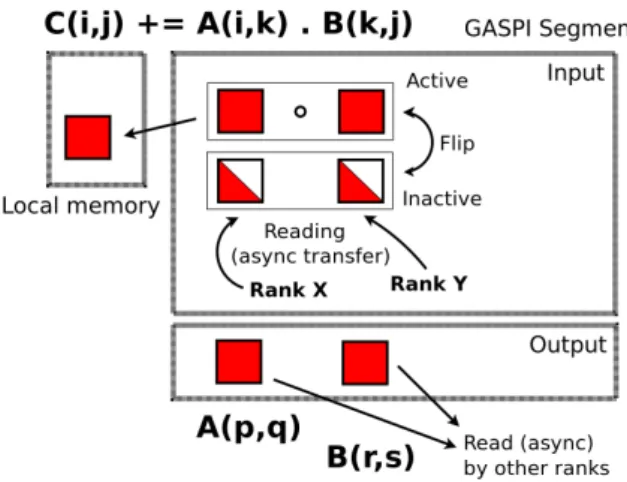
for any input blocking of matrices. This is achieved by using the double buffering approach which is described in the following: each rank has two sets of GASPI segments, first, or the ‘output’ segment serves for persistent storage of block(s) of matrices A and B, that other ranks can read without active participation of the ‘host’ rank. Second, it is the ‘input’ segment, which stores (temporarily) matrix blocks read from remote ranks (see Figure 1). Within the ‘input’ block of GASPI segments, one pair ofAand B blocks is active and one inactive
Fig. 1: Schema of GASPI matrix-matrix multiplication and memory layout on rank (parallel process).
at a time. ‘Active’ means that blocks contain all data and participate in local DGEMM operation i.e.in the computation, while ‘inactive’ labels the destination memory segment for asynchronous reads from remote ranks, i.e.it is used for communication. Once the local DGEMM computation and the communication with remote ranks is finished, active and inactive segments switch their role and the resultingC matrix block (stored in the local memory) is updated. That way the communication and the computation do not block each other.
The initial distribution of blocks can be chosen arbitrarily and, as shown further, has practically negligible effect on the overall timing. For a particular blocking and distribution of blocks (an example shown in Figure 2) a chain of (AIK, BKJ) block pairs is created for eachCIJ block, which must be multiplied and summed up. In certain stage of processing of the chain, a block of Aand/or B can already be present in the ‘output’
Fig. 2: Distribution of blocks of matricesA,B, andC across parallel processes (left), each rank being represented by different color. Overlap of computation (‘multiply’) and communication (‘read’) during parallel
execution of matrix multiplication (right) is demonstrated on two ranks.
segment of the rank, and does not need not to be transferred over the network. This can be utilized to increase efficiency of the first step of the chain, where communication is not overlapped by computation.
3.2. Results
In this section we benchmark our GASPI implementation with respect to the Intel MKL (Math Kernel Library) parallel matrix multiplication function - PDGEMM. For the sake of fair comparison, the initial partitioning (parallel distribution) of matrices was identical in both approaches. In the scope of this project, our GASPI algorithm is restricted to square matrices only. All timings presented throughout the text were obtained using
the ‘Anselm’ supercomputer cluster of IT4Innovations, National Supercomputing Center, VˇSB - Technical Uni-versity of Ostrava, Czech Republic. Each node consists of two 8-core Intel Sandy Bridge E5-2665 processors (2.4 GHz), nodes were connected with QDR Infiniband network (4 x QDR, 40 Gbps) with fully non-blocking fat-tree topology.
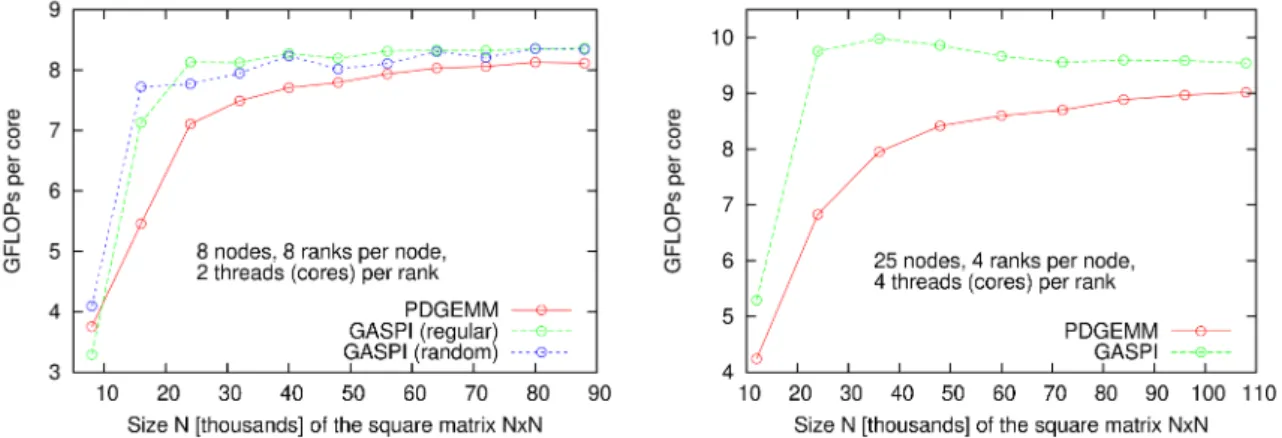
The first set of results demonstrates the performance of matrix multiplication for various matrix sizes. In analogy with serial matrix multiplication, where the size of multiplied matrices impacts the efficiency of utiliza-tion of (the hierarchy of) caches, we also analysed the minimum matrix dimension to allow for efficient overlap of computation and communication. Figure 3 depicts two such comparisons. The left chart shows GFLOPs per
Fig. 3: Scaling of GASPI and PDGEMM parallel matrix multiplication performance with respect to the size of matrices. To setups displayed: left - 8 nodes (64 ranks), right - 25 nodes (100 ranks). ‘Regular’ and ‘random’
GASPI implementations refer to assignment of matrix blocks to ranks: row-major or random order.
second per core on 8 nodes utilizing all (128) physical cores, using threaded (Intel MKL) DGEMM for local multiplication (2 threads per rank); the chart on the right shows results obtained on 25 nodes, all (400) cores, but 4 threads per rank. The number of operations is calculated as the cube of the matrix dimension, which is the number of double-precision multiplications that has to be carried out. Our GASPI algorithm, except for the smallest matrix size (N=8000) on 8 nodes, performs constantly better compared to PDGEMM, but the difference decreases with the size of matrices. This is not surprising, as the number of FLOPs increases with the third power of the matrix size, while the amount of transferred data with only the second power. GASPI performs notably better for matrices withN from 15 to 40K, and the difference is more obvious in larger parallel runs (more then 40% improvement). Comparing performance of two GASPI variants, ‘regular’ and ‘random’ (left chart), demonstrates another potentially advantageous feature: weak dependence on initial matrix blocks distribution among the ranks. In the ‘random’ approach, blocks of matricesA,B andC are randomly assigned to ranks (as e.g. in Figure 2), while in ‘regular’ approach (not necessarily optimal), blocks are distributed in row-major ordering. This ordering guarantees that at least one block of matrixA, needed for calculation of a block of matrixC, is stored on the same rank, thus does not need to be transferred over the network.
The next set of tests inspect the efficiency of our approach on SUMMA-like initial distribution of matrices. Splitting of blocks of multiplied matrices into smaller sub-blocks is used in SUMMA (thus in PDGEMM too) to achieve better parallelism. Such refined partitioning is beneficial to our GASPI algorithm as well, as it leads to a decrease of memory requirements, due to smaller buffers’ size. As shown in Figure 4 for 8 nodes (128 cores), two levels of blocking (‘blocking 2’ means splitting original blocks into 4 (22) identical squares; ‘blocking 4’, splitting into 16 (42) sub-blocks; etc.) have fairly small impact on the performance for matrices of sizes (N) from 8K to 90K. More refined, ‘level 8’ blocking (i.e.splitting original blocks into 64 (82) sub-blocks) leads to notable drop of performance, particularly for smaller matrices, N < 40K. Nevertheless, performance of ‘blocking 1’ (i.e.same number of blocks and ranks), except for the outlier - ‘blocking 2’ for N being 8K, is upper bound for more refined blocking. This is probably due to a synergic effect of the sufficient overlap of computation and communication, and efficiency of local DGEMM operations for larger blocks.
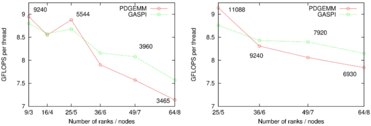
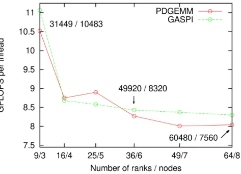
The last series of tests demonstrate strong- and weak parallel scaling. Strong scaling, shown in Figure 5, is parallel scaling for a fixed matrix size and an increasing number of parallel processes, while weak scaling (see Figure 6) reflects the performance change for constant work load per parallel process with increasing number of ranks. In both cases we systematically increase the number of nodes (and ranks) according to SUMMA-like concept of the so-called processing grid. We utilize square processing grids of dimension 2 (4 ranks), 3 (9 ranks), etc., which is deliberately equal to the number of nodes. To have an equal distribution of ranks among nodes, each node has as many ranks as the dimension of the processing grid, i.e.2 nodes, 2 ranks per node; 3 nodes, 3 ranks per node,etc..
Let us discuss the strong scaling results first. The left chart in Figure 5 depicts strong scaling results for a small matrix (N being 27 720), from 3 to 8 nodes, or 9 to 64 ranks respectively, each rank utilizing 2 threads
Fig. 4: Scaling of GASPI parallel matrix multiplication performance with respect block- and total size of (square) matrix, on 64 ranks (8 nodes, 8 ranks per node and 2 threads per rank). ‘Blocking 1’ means equal number of blocks (NB) and ranks (NR), ‘Blocking 2’ corresponds to splitting each block into four blocks,etc.,
as schematically shown in the graphics for 4 ranks.
in local DGEMM. The block size is quite large for runs a with small number of ranks,e.g.9240 for 3 nodes (9 ranks). The GASPI computation on one node with two ranks (block size of 13 860) was crashing, unlike the PDGEMM. Furthermore, the PDGEMM seems to outperform GASPI up to 5 nodes, but the opposite is true from 6 nodes on. Similar trends can be observed for a larger matrix (chart on the right in Figure 5), N being 55 440. Performance on 1 to 3 nodes is omitted, because both GASPI and PDGEMM runs crashed. Four-nodes run is omitted, because of failure of the GASPI code only. GASPI delivers slightly more GFLOPS compared to PDGEMM on six nodes and more.
Weak scaling is analyzed for a series of matrix sizes from ∼30K to 60K, using 3 to 8 nodes. The block-and the total matrix size for each processing grid was obtained using equationNB(2)∗p3 p
2/pi, whereNB(2) is the ‘input’ block size (of 12K, in this case) for a matrix and processing grid of dimension 2 (i.e.p2), and
pi is the dimension of target processing grid (3, 4, etc.). The total size (N) of matrix is then pi ∗ NB(i). GASPI computation on smaller number of nodes failed, probably due to large block sizes. Performance of both algorithms on 3 to 5 nodes is quite erratic, however, starting from 6 nodes on GASPI performs slightly better, though the difference is on the order of (a few) percents.
Fig. 5: Strong scaling of GASPI and PDGEMM parallel matrix multiplication. Matrix size (N) is 27 720 (left) and 55 440 (right). Numbers in charts (above data points) indicate size of blocks, upon matrix partitioning.
Fig. 6: Weak scaling of GASPI and PDGEMM parallel matrix multiplication. Numbers in the charts indicate size of matrix / block for selected values.
4. Machine Learning Algorithms
A collection of a large variety of algorithms for regression, classification, clustering,etc., often originated from fields like statistics or optimization, are referred to as the ‘machine learning’ algorithms. These algorithms are used for prediction, either based on training on known outputs ((semi-)supervised learning) or without (unsupervised learning). The widespread adoption of machine learning became possible thanks to synergy of several developments: large amounts of available data (i.e. ‘Big data’) on which such algorithms strive, computing power of commodity hardware and availability of easy to use software tools, that can aggregate the computing power of the (commodity) cluster nodes. The JVM-based parallel frameworks like Apache Hadoop (and its modules MapReduce, HDFS) and Apache Spark paved the way to large-scale machine learning applications on data sizes in terabytes (and beyond), without a need for supercomputers and knowledge of MPI. These frameworks offer an unprecedented level of abstraction towards parallel computing, user-friendliness by APIs in programming languages like Java or Python, runtime resilience out-of-the-box,etc. Thanks (in part) to these frameworks, a tremendous number of machine learning / AI applications have been developed, that occupy more and more HPC resources nowadays. However, JVM-based frameworks inevitably come with an extra software layer and other ‘features’ (e.g. garbage collection memory management), that may negatively affect the performance of the applications [15, 16]. The goal of this part of the mini-project is to converge big data and traditional HPC approaches. While techniques from HPC should clearly outperforms JVM-based frameworks in terms of performance, special care needs to be taken to incorporate runtime resilience in the traditional HPC approaches.
4.1. K-means
K-means is a relatively simple, yet powerful and popular clustering machine learning algorithm used in classifica-tion, segmentaclassifica-tion, feature learning, image compression,etc. The goal is to partition observations S (typically,
n-dimensional vectors) intokdistinct sets, each represented by its centroid (not necessarily one of the observa-tions). Observations are partitioned so that the squared distance between cluster members and the centroid is minimal: min k X i=1 X ¯ xj∈Si kx¯j−µ¯ik2 (2)
where Si is the set of observations ¯xj in clusteri, and ¯µi is its centroid. To find the exact minimum of this function is an NP-hard problem, thus in real-life applications we rely on a solution obtained using this algorithm:
0. Selectkinitial centers
1. Generate partitioning by assigning observations to the closest centroid. If the cluster membership changed, go to next step, otherwise finish.
The parallel implementation of this algorithm is straightforward: observations are split among the ranks; in each iteration the algorithm assigns the cluster membership for local observations to a rank and calculates its contribution to centroid coordinates (keeping track of the contributing observations count). At the end of each iteration, the ranks on the nodes exchange information calculated locally to eventually obtain new centroid coordinates. The most straightforward and probably the most efficient implementation is calling the ‘allreduce’ collective operation, which is highly optimized for the communication bandwidth. We have also implemented MPI and GASPI versions of the algorithm without use of blocking collective operations. We utilized instead ‘reduce and broadcast’ combinations of MPI Isend and MPI Recv, in the case of MPI, or gaspi write notify and gaspi notify waitsome / gaspi notify reset, in the case of GASPI, but without noteworthy impact on the performance.
In the K-means algorithm each rank has relatively little computation to carry out, and has to frequently exchange data (not necessarily directly) with all other ranks. It is thus no surprise, that an efficient data-dependency driven (i.e. without global barriers), asynchronous parallel implementation is almost impossible to conduct. The JVM K-means implementations, as reported by Kamburugamuve et al. [16], though being clearly slower, perform reasonably well (i.e.timings at the same order of magnitude) compared to the MPI. Nevertheless, we can still use the K-means algorithm to demonstrate GASPI fault tolerance capabilities.
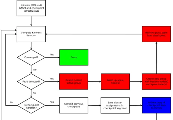
Our GASPI K-means implementation achieves run-time resilience using two fundamental concepts: timeout of communication operations, and the error state vector. In the asynchronous programming model GASPI, global (typically blocking) operations, such as barrier or allreduce can be provided with the finite timeout value. Should the operation time out, faulty rank(s) can be identified by calling gaspi state vec get, which returns a vector of values GASPI STATE HEALTHY and GASPI STATE CORRUPT for each rank. If a fault state is detected, the application enters recovery mode. Recovery is typically application specific, in our case we opted for non-shrinking restart (i.e.utilizing spare node(s)) from saved centroid coordinates, with the help of in-memory checkpointing library (GPI CP) [6]. This library automates the process of creating checkpoints
Fig. 7: Flow diagram of the fault-tolerant K-means implementation using (red indicates fault recovery sequence, blue is asynchronous step).
and hides the overhead due to checkpoint distribution to mirrors via asynchronous GASPI communication. As shown in Figure 7, this is a two step procedure. First, the checkpoint is ‘started’, which means that the ranks in-volved initiate asynchronous copying of data to neighboring mirrors (e.g.in ring topology). In the second stage, checkpoint is ‘committed’, which is a global operation to ensure that all participating ranks have a consistent copy of the data. This gpi cp commit operation itself is non-blocking, takes a timeout parameter, and can be ‘tested’ on completion in order to decide on creating a new checkpoint. Hiding of checkpoint creation overhead can be naturally achieved by specifying a reasonable frequency of checkpointing,e.g.each 50th iteration of the K-means procedure, in our case. It is also worth noting, that despite being an in-memory checkpointing library, checkpoint persistence can be achieved by utilizing non-volatile (e.g. NVRAM) memory devices.
Table 1 summarizes the timings of 500 iterations of parallel K-means run for 1 million 10-dimensional points and 1000 centroids, with four parallel processes per node. The frequency of creating checkpoints (after each 50
Table 1: Timing [s] of K-means parallel run. The ‘CP commit’ corresponds to total time spent in committing of checkpoints (created asynchronously) after each 50 iterations. ‘Recovery’ corresponds to the overhead due to reconstructing of the GASPI processors group and checkpoint loading after killing one randomly selected rank during the application run.
Nodes Total run CP commit Recovery
4 150 0.06 0.45
8 72 0.15 0.62
12 50 0.17 0.71
16 37 0.25 0.79
iterations) is sufficiently large to hide the overhead of the backup process, as can be concluded from timings on the order of fractions of a second. The overhead due to the recovery process, measured by killing a randomly chosen rank once during the application run, represents 0.2 to 2.1% of the total wall-clock time, and naturally increases with the number of parallel processes.
4.2. Terasort
Terasort (i.e. Terabyte sort) is a popular algorithm for sorting large files in parallel. The central idea of the algorithm, depicted in Figure 8, is to distribute the sorting workload among multiple nodes via partitioning of the large input file using a ‘hash function’. Partitions are collected from all ranks, sorted locally (in parallel),
Fig. 8: Asynchronous communication between ranks A and B in the GASPI Terasort implementation.
and written to the output file. The role of the hash function is to assign, which partition each sorted element belongs to, and its design is, in general, problem-specific. A generic approach is to collect samples of the sorted data, ideally from all (or at least multiple) parallel ranks, and set up the hash function to partition sample data. Presuming the samples represent the sorted data reasonably well, and the rest of the data is distributed evenly across the ranks, this is a viable approach.
The Terasort algorithm follows the ‘two-step’ programming principles of Hadoop MapReduce and takes great advantage of data locality in HDFS. A file deployed to HDFS is automatically split into chunks (with redundancy,i.e.two- or more replicas of each chunk exists across the HDFS cluster), which are stored locally. When a file is processed using MapReduce, chunks are read from the local drives, which leads to excellent aggregate I/O performance, even on commodity hardware. The bottleneck of Terasort is, however, shuffling of data among the parallel nodes.
In this work we compare two implementations: MPI implementation with a global barrier prior to data shuf-fling and asynchronous, data-dependency driven GASPI implementation. In both cases we use an in-memory approach, meaning that enough aggregate RAM on the ranks must be available to store the input data. The MPI algorithm is simpler, and works as follows: first, the input data is read in parallel using the MPI-IO collective function MPI File read at all. Next, each rank evaluates partitioning according to sampled data and exchanges this information with other ranks. Data is then locally partitioned and after reaching the global barrier, data shuffling (using MPI Isend and MPI recv) is initiated. Once each rank receives all data of its partition, local sorting (qsort function) is initiated and the sorted data is written to the output file.
The GASPI algorithm is slightly more elaborate. While reading data and setting up partitions is identical with the MPI implementation, the shuffling phase is completely different. Each rank has two GASPI segments: one is the ‘output’ segment, and it is split into 2(N−1) buffers, whereNis the number of ranks. The other one is the ‘input’ segment, and has onlyN−1 buffers. Communication between two ranks, A and B, is depicted in Figure 9. While processing its local data, rank A assigns data to belong to,e.g.partition of rank B, and appends
Fig. 9: Asynchronous communication between ranks A and B in the GASPI Terasort implementation.
it to one of ‘output’ buffers designated for rank B. When the buffer is full, rank A initiates asynchronous copy of the buffer to rank B and continues using the other (empty) output buffer for rank B (this explains 2(N−1) buffers). Rank B periodically checks for new notification on input segments, detects the input buffer from rank A is full, and copies the data to local memory (array of pointers). Next the input buffer is emptied and rank A is notified that rank B is ready to receive new data whenever needed. If rank A does not receive this notification, it will not initiate new transfers to rank B.
Before we could compare the two implementations, we needed to find suitable value for the buffers’ size. Experiments on 2 nodes (24 ranks) and 36 GB of data revealed, that among the buffer lengths from 1K to 60K, value 10K performed the best. Concerning the type of sorted data, our first implementations targeted integers and real numbers, in combination with radix sort for local data sorting. For the sake of seamless comparison with other approaches, we switched to so-called ‘Indy’ format [17] used at http://sortbenchmark.org. Records consist of a fixed size, 10 byte random key (string) and 90 bytes of random data (string), so the total record length is 100 bytes.
Figure 10 depicts the comparison of strong and weak scaling of MPI and GASPI implementations. Tim-ings cover only the data shuffle phase. We believe this is fair comparison, because other phases, such as data sampling (i.e.partitions setup) or local sorting, are either identical in both implementations, or perform unpre-dictably, such as MPI-IO read of input data, and the MPI-IO write of a sorted file. The advantage of GASPI
Fig. 10: Strong (left) and weak scaling (right) of the shuffle phase of MPI and GASPI Terasort implementations, in GBs of sorted data per second per node. Strong scaling is shown for 60 GB file, weak
scaling for files from 60 to 240 GB, on 2 to 8 nodes (32 to 128 ranks).
to 4 nodes), as can be seen on the strong scaling chart (Figure 10, left), or across the whole weak scaling chart (right). The two approaches perform equal for the large number of ranks and (relatively) small input data size. We did not implement a fault tolerant version of the Terasort algorithms. We could not find a recovery strategy that would be significantly more efficient than restarting the whole application. To be more specific, we could not find a way to recover, should the failure occur in the shuffle phase. This is not specific to MPI or GASPI; the Apache Spark implementation also pays high penalty (comparable to the cost of the application restart) in case of failure in shuffle phase. This is an example of the aforementioned ‘wide dependency’ of RDDs. The whole shuffle phase (including reading of input data, if not cached) has to be repeated on all parallel processes to recover from failure. Recovery in our GASPI implementation (in, e.g. non-shrinking recovery strategy) could follow these steps: all healthy nodes clean their input buffers and local memory segments, that correspond to the failed rank. A spare node then redistributes its local input data to other ranks again, but recreating its own input buffers would require all other nodes to re-read the whole input data, and resend the partition of the failed rank.
5. Conclusion
It this work we summarize our experience with the PGAS programming model GASPI for building highly scal-able, parallel and fault tolerant HPC applications. We have implemented GASPI and MPI versions of selected algorithms relevant in both the HPC realm (e.g. computational quantum chemistry) and the ‘Big Data world’, that has lately made its way to supercomputers. We utilized the GASPI asynchronous, one-sided operations to overlap computation and communication, its interoperability with MPI to use MPI-IO for efficient I/O opera-tions on Lustre parallel file system, and its timeout mechanism to detect and recover from node(s) failure. All these GASPI features are essential for a programming tool with ambition to utilize the full potential of future Exascale systems.
The GASPI implementation of parallel matrix multiplication (or tensor contraction) is competitive with the state-of-the-art parallel DGEMM function distributed with Intel MKL package. Performance using a large num-ber of parallel processes seems to be even superior to PDGEMM, but more precise and extensive benchmarking is required. Wall-clock timings may be sensitive to particular assignment of ranks to physical nodes, topology of underlying network and its utilization during tests. The GASPI program itself is remarkably simple, and uses collective or blocking operations only marginally.
Two selected machine learning algorithms, K-means and Terasort, were implemented using MPI and GASPI. In the case of K-means, we also implemented its fault tolerant version with non-shrinking recovery strategy and checkpointing, made simple by GPI CP library. Similarly to parallel matrix multiplication implementation, timings obtained for the GASPI code indicate better parallel scaling, especially for larger number of ranks. We have addressed two of three outstanding features of JVM Big data frameworks (such as the Apache Spark), that are not readily provided by MPI: fault tolerance and utilization of parallel (fault tolerant) file systems (Lustre instead of HDFS). The last, but certainly not least advantage ofe.g.Apache Spark remained undaunted: easy of use. Despite that GASPI provides a truly straightforward (minimum boilerplate) approach to asynchronous PGAS HPC programming, its performance benefits may not be enough to motivate developers to sacrifice high-level abstractions, such as RDDs. Retaining the high productivity of developers, while keeping the perfor-mance benefits of MPI/GASPI, is not only desirable but seems to be possible too, as shown by several hybrid approaches, such as GPI-Space or Spark+MPI [18].
Acknowledgements
This work was financially supported by the PRACE project funded in part by the EUs Horizon 2020 Re-search and Innovation programme (2014-2020) under grant agreement 730913. This work was also supported by The Ministry of Education, Youth and Sports of the Czech Republic from the Large Infrastructures for Research, Experimental Development and Innovations project ‘IT4Innovations National Supercomputing Cen-ter LM2015070’. Parts of the computations were performed in the High-Performance Computing Center, Centre of Operations of the Slovak Academy of Sciences using the HPC infrastructure acquired in project ITMS 26230120002 and 26210120002 (Slovak Infrastructure for High-Performance Computing) supported by the Research & Development Operational Programme funded by the ERDF.
References
1. Wesley Bland, Aurelien Bouteiller, Thomas Herault, Joshua Hursey, George Bosilca, and Jack J. Don-garra. An evaluation of user-level failure mitigation support in mpi. Computing, 95(12):1171–1184, December 2013.
2. Ignacio Laguna, David F. Richards, Todd Gamblin, Martin Schulz, and Bronis R. de Supinski. Evaluating user-level fault tolerance for mpi applications. In Proceedings of the 21st European MPI Users’ Group Meeting, EuroMPI/ASIA ’14, pages 57:57–57:62, New York, NY, USA, 2014. ACM.
3. Ignacio Laguna, David F Richards, Todd Gamblin, Martin Schulz, Bronis R de Supinski, Kathryn Mohror, and Howard Pritchard. Evaluating and extending user-level fault tolerance in mpi applications. The International Journal of High Performance Computing Applications, 30(3):305–319, 2016.
4. Christian Simmendinger, Mirko Rahn, and Daniel Gruenewald. The gaspi api: A failure tolerant pgas api for asynchronous dataflow on heterogeneous architectures. In Michael M. Resch, Wolfgang Bez, Erich Focht, Hiroaki Kobayashi, and Nisarg Patel, editors, Sustained Simulation Performance 2014, pages 17–32, Cham, 2015. Springer International Publishing.
5. Daniel Gr¨unewald and Christian Simmendinger. The gaspi api specification and its implementation gpi 2.0. In Proceedings of the 7th International Conference on PGAS Programming Models. University of Edinburgh, 2013.
6. Valeria Bartsch, Rui Machado, Dirk Merten, Mirko Rahn, and Franz-Josef Pfreundt. Gaspi/gpi in-memory checkpointing library. In Francisco F. Rivera, Tom´as F. Pena, and Jos´e C. Cabaleiro, editors, Euro-Par 2017: Parallel Processing, pages 497–508, Cham, 2017. Springer International Publishing. 7. Tiberiu Rotaru, Mirko Rahn, and Franz-Josef Pfreundt. Mapreduce in gpi-space. In Dieter an Mey,
Michael Alexander, Paolo Bientinesi, Mario Cannataro, Carsten Clauss, Alexandru Costan, Gabor Kecskemeti, Christine Morin, Laura Ricci, Julio Sahuquillo, Martin Schulz, Vittorio Scarano, Stephen L. Scott, and Josef Weidendorfer, editors,Euro-Par 2013: Parallel Processing Workshops - BigDataCloud, DIHC, FedICI, HeteroPar, HiBB, LSDVE, MHPC, OMHI, PADABS, PROPER, Resilience, ROME, and UCHPC 2013, Aachen, Germany, August 26-27, 2013. Revised Selected Papers, volume 8374 of Lecture Notes in Computer Science, pages 43–52. Springer, 2013.
8. Rodney J. Bartlett and Monika Musia l. Coupled-cluster theory in quantum chemistry. Rev. Mod. Phys., 79:291–352, Feb 2007.
9. M. Valiev, E. J. Bylaska, N. Govind, K. Kowalski, T. P. Straatsma, H. J. J. Van Dam, D. Wang, J. Nieplocha, E. Apra, T. L. Windus, and W. A. de Jong. NWChem: A comprehensive and scalable open-source solution for large scale molecular simulations.Computer Physics Communications, 181:1477–1489, September 2010.
10. So Hirata. Tensor contraction engine: abstraction and automated parallel implementation of configuration-interaction, coupled-cluster, and many-body perturbation theories. The Journal of Phys-ical Chemistry A, 107(46):9887–9897, 2003.
11. Edgar Solomonik, Devin Matthews, Jeff R. Hammond, John F. Stanton, and James Demmel. A mas-sively parallel tensor contraction framework for coupled-cluster computations. Journal of Parallel and Distributed Computing, 74(12):3176 – 3190, 2014. Domain-Specific Languages and High-Level Frame-works for High-Performance Computing.
12. D. Matthews. High-performance tensor contraction without transposition. SIAM Journal on Scientific Computing, 40(1):C1–C24, 2018.
13. R. A. Van De Geijn and J. Watts. Summa: scalable universal matrix multiplication algorithm. Concur-rency: Practice and Experience, 9(4):255–274, 1997.
14. Manojkumar Krishnan and Jarek Nieplocha. Srumma: a matrix multiplication algorithm suitable for clusters and scalable shared memory systems. 18th International Parallel and Distributed Processing Symposium, 2004. Proceedings., pages 70–, 2004.
15. Jorge L. Reyes-Ortiz, Luca Oneto, and Davide Anguita. Big data analytics in the cloud: Spark on hadoop vs mpi/openmp on beowulf. Procedia Computer Science, 53:121 – 130, 2015. INNS Conference on Big Data 2015 Program San Francisco, CA, USA 8-10 August 2015.
16. Supun Kamburugamuve, Pulasthi Wickramasinghe, Saliya Ekanayake, and Geoffrey C. Fox. Anatomy of machine learning algorithm implementations in mpi, spark, and flink. IJHPCA, 32:61–73, 2018. 17. GNU. Gensort data generator, v.1.5. http://www.ordinal.com/gensort.html. Accessed: 2019-02-21. 18. Michael Anderson, Shaden Smith, Narayanan Sundaram, Mihai Capot˘a, Zheguang Zhao, Subramanya Dulloor, Nadathur Satish, and Theodore Willke. Bridging the gap between hpc and big data frameworks. InProceedings of the 43rd International Conference on Very Large Data Bases, Proceedings of the VLDB Endowment, pages 901 – 912, 2017.
![Table 1: Timing [s] of K-means parallel run. The ‘CP commit’ corresponds to total time spent in committing of checkpoints (created asynchronously) after each 50 iterations](https://thumb-us.123doks.com/thumbv2/123dok_us/9901520.2483547/9.892.248.645.530.673/timing-parallel-corresponds-committing-checkpoints-created-asynchronously-iterations.webp)

