A recurrent neural network architecture for biomedical event trigger classification

University of Kentucky University of Kentucky

UKnowledge

UKnowledge

2018

A recurrent neural network architecture for biomedical event

A recurrent neural network architecture for biomedical event

trigger classification

trigger classification

University of Kentucky, [email protected] Author ORCID Identifier:

https://orcid.org/0000-0001-8046-6289

Digital Object Identifier: https://doi.org/10.13023/etd.2018.369

Right click to open a feedback form in a new tab to let us know how this document benefits you. Right click to open a feedback form in a new tab to let us know how this document benefits you.

Recommended Citation Recommended Citation

Bopaiah, Jeevith, "A recurrent neural network architecture for biomedical event trigger classification" (2018). Theses and Dissertations--Computer Science. 73.

https://uknowledge.uky.edu/cs_etds/73

This Master's Thesis is brought to you for free and open access by the Computer Science at UKnowledge. It has been accepted for inclusion in Theses and Dissertations--Computer Science by an authorized administrator of

STUDENT AGREEMENT: STUDENT AGREEMENT:

I represent that my thesis or dissertation and abstract are my original work. Proper attribution has been given to all outside sources. I understand that I am solely responsible for obtaining any needed copyright permissions. I have obtained needed written permission statement(s) from the owner(s) of each third-party copyrighted matter to be included in my work, allowing electronic distribution (if such use is not permitted by the fair use doctrine) which will be submitted to UKnowledge as Additional File.

I hereby grant to The University of Kentucky and its agents the irrevocable, non-exclusive, and royalty-free license to archive and make accessible my work in whole or in part in all forms of media, now or hereafter known. I agree that the document mentioned above may be made available immediately for worldwide access unless an embargo applies.

I retain all other ownership rights to the copyright of my work. I also retain the right to use in future works (such as articles or books) all or part of my work. I understand that I am free to register the copyright to my work.

REVIEW, APPROVAL AND ACCEPTANCE REVIEW, APPROVAL AND ACCEPTANCE

The document mentioned above has been reviewed and accepted by the student’s advisor, on behalf of the advisory committee, and by the Director of Graduate Studies (DGS), on behalf of the program; we verify that this is the final, approved version of the student’s thesis including all changes required by the advisory committee. The undersigned agree to abide by the statements above.

Jeevith Bopaiah, Student Dr. Ramakanth Kavuluru, Major Professor Dr. Mirosław Truszczyński, Director of Graduate Studies

A recurrent neural network architecture for biomedical event trigger classification

THESIS

A thesis submitted in partial fulfillment of the requirements for the degree of Master of Science in the College of Engineering at the

University of Kentucky By

Jeevith Bopaiah Lexington, Kentucky

Director: Dr. Ramakanth Kavuluru Lexington, Kentucky 2018

ABSTRACT OF THESIS

A recurrent neural network architecture for biomedical event trigger classification A “biomedical event” is a broad term used to describe the roles and interactions be-tween entities (such as proteins, genes and cells) in a biological system. The task of biomedical event extraction aims at identifying and extracting these events from unstructured texts. An important component in the early stage of the task is biomed-ical trigger classification which involves identifying and classifying words/phrases that indicate an event. In this thesis, we present our work on biomedical trigger classifica-tion developed using themulti-level event extraction dataset. We restrict the scope of our classification to 19 biomedical event types grouped under four broad categories -Anatomical, Molecular, General and Planned. While most of the existing approaches are based on traditional machine learning algorithms which require extensive feature engineering, our model relies on neural networks to implicitly learn important features directly from the text. We use natural language processing techniques to transform the text into vectorized inputs that can be used in a neural network architecture. As per our knowledge, this is the first time neural attention strategies are being explored in the area of biomedical trigger classification. Our best results were obtained from an ensemble of 50 models which produced a micro F-score of 79.82%, an improvement of 1.3% over the previous best score.

KEYWORDS: LSTM, word embeddings, biomedical triggers, attention layer

Author’s signature: Jeevith Bopaiah

A recurrent neural network architecture for biomedical event trigger classification

By

Jeevith Bopaiah

Director of Thesis: Ramakanth Kavuluru Director of Graduate Studies: Mirosław Truszczyński

ACKNOWLEDGMENTS

In the last few years, I have met some wonderful people who have had a profound impact on my personal and professional life. My journey as a master’s student would not have been the same without these people.

First of all, I would like to express my gratitude to Dr. Ramakanth Kavuluru for his guidance and support throughout the program. His constructive feedbacks on my research work have helped me improve my conceptual understanding and technical writing abilities. He always encouraged me to strive for the best and took an active interest in my job search. I am really fortunate to have had him as the thesis advisor for my master’s program.

I am grateful to Dr. Sally Ellingson for giving me the opportunity to work on one of her research projects. This project gave me a platform to hone my data engineering skills. My first work assignment at the university was with the Research Information Services department. A big thank you to William Clark for his support and guidance during the assignment.

My sincere thanks to the committee members Dr. Jerzy Jaromczyk and Dr. Licong Cui for providing valuable feedback which helped me in improving this thesis. A special thanks to Dr. Jerzy Jaromczyk for being instrumental in making this journey a reality. A special mention to my mentor and guide, Vijaykant Nadadur. He has been a role model in many ways and it was his encouragement that brought me here to the master’s program.

I would like to thank my friends, Arjun Nagaraj and Sagar Rao for always being there for me when I needed them. Lastly, a big thank you to my parents for their constant love and support.

TABLE OF CONTENTS

Acknowledgments . . . iii

Table of Contents . . . iv

List of Tables . . . vi

List of Figures . . . vii

Chapter 1 Introduction . . . 1

1.1 What is Biomedical Natural Language Processing? . . . 1

1.2 Biomedical Event Extraction . . . 3

1.3 Biomedical Event Trigger Classification . . . 4

Chapter 2 Related Work . . . 6

Chapter 3 Dataset . . . 10

Chapter 4 Methods . . . 12

4.1 Preprocessing . . . 13

4.2 Bidirectional LSTM with attention . . . 14

4.2.1 Input embeddings . . . 15

4.2.2 Stacked BiLSTM layer . . . 16

4.2.3 Attention layer . . . 17

4.2.4 Feature Engineering . . . 17

Chapter 5 Experiments and Results . . . 19

5.1 Experiments . . . 19 5.2 Results . . . 20 5.2.1 Model Ensembles . . . 21 5.2.2 Ablation Study . . . 21 5.3 Analysis . . . 22 Chapter 6 Reproducibility . . . 24 6.1 Abstract Preprocessing . . . 25 6.2 Negative Filtering . . . 25 6.3 External Features . . . 26 6.4 Input Data . . . 27 6.5 Classifier . . . 27 6.6 Training . . . 28 6.7 Testing . . . 29 Chapter 7 Conclusion . . . 30

7.1 Limitations . . . 30

7.2 Future Work . . . 30

Bibliography . . . 32

LIST OF TABLES

3.1 Distribution of Event Types . . . 10

3.2 Distribution of Entity Types . . . 11

4.1 Valid Semantic Types . . . 14

4.2 Data summary before and after candidate filtering process . . . 14

5.1 Comparison of our model against prior works . . . 21

LIST OF FIGURES

1.1 Data Samples . . . 5

4.1 Event Trigger Classification Framework . . . 15

5.1 Error patterns . . . 23

Chapter 1 Introduction

Natural language processing (NLP) is an interdisciplinary area of research that lies at the intersection of linguistics and computer science [1]. On a macro level it attempts to build applications and tools that can understand and interpret language to perform useful tasks. Unlike programming languages and other symbolic languages useful for specialized domain specific communication, natural language involves complex syn-tactic and semantic structure and a loosely defined grammar to enable creative use of the language. This variability in linguistic structure and flexibility of its associated grammar makes processing natural language more difficult compared to artificial lan-guages. With the proliferation of unstructured content on digital platforms, there is a need for NLP systems that can manage huge volumes of textual data and de-rive actionable insights from them. Recent advances in computing resources, growing potential of unstructured data and its widespread use in various domains has not only encouraged traditional NLP research but also provided a strong foundation for domain specific NLP systems.

1.1 What is Biomedical Natural Language Processing?

A vast majority of biomedical knowledge ranging from scientific research papers to patient related data are expressed in natural language text. Physicians and other med-ical researchers read through these verbose textual data to mine important biomedmed-ical facts and findings. With the increasing growth in biomedical literature, manual ex-ploration of these articles became a herculean task. The need for an automated or machine assisted processing of the texts was increasingly felt by the biomedical community which led to the development of a subfield in NLP known as biomedical NLP (BioNLP). BioNLP [2, Chapter 2] is the application of NLP techniques to de-rive meaningful and actionable information from biomedical text such as electronic medical records and biomedical literature. Domain specific applications are some-what different from traditional language processing tasks. Even though there is a considerable overlap between traditional and biomedical NLP, there are several tasks that are specific to biomedical field which require different strategies. Most of these tasks are driven by the needs of the physicians and medical practitioners who also happen to be the primary users of these systems. Besides the tasks that have end user applications, there also exists certain NLP tasks that form intermediary

com-ponents in a larger system. One such example is word sense disambiguation [3, 4] which resolves ambiguities in the contextual meaning of the word, especially when the same word assumes multiple meanings. The flexibility of a language allows the use of different linguistic expressions to refer to the same biomedical concept. To re-duce the variability in expression and provide a universal representation of a concept, concept normalization [2, Chapter 6] task was introduced to map each concept in the text to a unique concept identifier. Named entity recognition [2, Chapter 3] (NER) is also a well known language processing task with an objective to identify entities (such as proteins, genes and cells) in unstructured texts. The entity names/types allow us to generate a higher level and more generalized representation of the text. A natural extension of NER is the extraction of relationships between the entities [2, Chapter 4], [5]. These relations describe the function and behavior of the entities which are of interest to knowledge base curators. This knowledge base of biomedical facts can assist healthcare professionals in making an informed clinical decision on their subjects.

Biomedical event extraction [6, 7] is a more complex type of relation extraction. Unlike relation extraction, whose focus is on binary relations, event extraction en-compasses extracting n-ary and even nested relations. Another area that is much appreciated by the medical community is automatic text summarization [2, Chapter 8]. Text summarization aims to extract the important details of a biomedical article or clinical notes of a patient and present it in a concise and coherent manner. De-pending on their purpose, the summaries can either be generic or targeted. While a generic summary presents the user with all the relevant facts, a targeted summary contains the details regarding a specific information need. Especially, doctors find this tool useful as the patient information from different sources can be summarized and presented in the form of facts, graphs and charts. Biomedical question answer-ing [2, Chapter 9] task was introduced with an aim to assist researchers and clinical practitioners in their search for specific biomedical facts. It was popularized by the BioASQ Challenge [8] which involved retrieving relevant articles for each question from a corpus of several thousand documents. Subsequently, depending on the spe-cific requirements, the system can be designed to generate either factoid answers, answer snippets, and list (of factoids) or summary type answers. Another important contribution of NLP in healthcare is in clinical decision support (CDS) systems. A CDS system draws the attention of health professionals towards patient specific events and also recommends suitable interventions. NLP techniques are used to process clin-ical narratives and monitor the likelihood of occurrence of an event. Some examples

include early identification of sepsis patients [9] and detection of post-surgical site infections [10]. The immense potential of NLP in biomedicine comes with its own set of challenges, most important being data annotation. Most of the tasks men-tioned here require annotated data to employ supervised statistical NLP techniques. Data annotation is an expensive, time-consuming process and it requires biomedical experts. To make effective use of the limited annotated data and facilitate research in bioNLP, several shared tasks are organized by the biomedical community. These shared tasks have played an important role in advancing the existing techniques and developing new state of the art systems for improving the quality of healthcare.

1.2 Biomedical Event Extraction

Over the last decade, scientific community has witnessed huge investments in biomed-ical research leading to improved diagnostic and therapeutic procedures. Conse-quently, this growing impetus in biomedical research has created a wealth of infor-mation in biomedical literature hosted in the PubMed search engine by the NIH. Among other research findings and experiments, these scientific articles also contain information on various biological events, which describe the behavior of an entity in the presence of other biomolecular entities or external substances such as chemical compounds. These events help physicians, clinical practitioners, and basic scientists understand the molecular interactions and keep themselves abreast with the new de-velopments in biomedicine. Although scientific literature constitutes a rich source of information on various biological processes and events, its effective utilization is ham-pered by the need to scour through the entire literature to locate relevant biomedical events. It is estimated that more than 7.3 million journal articles were added to PubMed repository in the period 2004-2013 which was an increase of 48.9% since 2003 [11]. As of now, PubMed hosts over 27 million biomedical citations (titles, abstracts, and other metadata).

Biomedical event extraction (BEE) is the process of extracting evidences of molec-ular interactions from scientific articles. A biomedical event is comprised of three parts: event trigger word, entities participating in the event, and role of each par-ticipating entity. NLP is used to process the text and extract the features that can be used by a machine learning algorithm to identify event structures in a piece of text. BEE was introduced for the first time through the BioNLP-ST’09 [12] com-munity shared task, where the entities participating in the event were restricted to protein and genes. In subsequent years, the scope of event extraction was increased

through shared tasks BioNLP-ST’11 [13] and BioNLP-ST’13 [14] to include chemical and cellular component entities participating in 19 different event types. The avail-ability of annotated data for public use has encouraged many researchers to develop event extraction systems pushing the boundaries of NLP and machine learning tech-niques. Some of the popular approaches to this task include Bui et al. [15], Björne et al. [6], and Li et al. [16]. Bui et al. [15] used a simple rule based approach to extract events from PubMed abstracts. They used the training data to generate lin-guistic patterns around trigger words and these patterns were applied on the test set to identify the presence/absence of an event and also to classify the event structure into one of the predefined event types. Björne et al. [6] employed machine learning techniques to train a multi class support vector machine (SVM). The features to the classifier included token features, sentence features, dependency parses, trigger fea-tures and external feafea-tures. The feafea-tures were converted to a vector of binary values indicating the presence or absence of the feature. Li et al. [16] used a neural network architecture composed of bidirectional long short-term memory (LSTM) units with dynamic extended tree of the sentence as its input. Computational techniques used by the prior works fall into three broad categories — rule based strategies which rely on well defined rules to identify the event patterns, machine learning techniques which involve learning the event patterns through the features provided to the model, and deep neural network architectures which avoid feature engineering and learn to identify the features directly from the text. Due to the complexity of BEE and the number of components (triggers, entities, arguments) involved, prior works can be broadly categorized into pipeline based approaches and joint model approaches. Pipeline based approaches model the individual components in a sequential manner while joint modeling approaches extract the entire event structure in a single input– output pass. Previous studies [17], have found that pipeline based strategies perform better than joint modeling approaches in BEE task. Therefore, in this thesis we focus on the first component of the pipeline, biomedical trigger classification.

1.3 Biomedical Event Trigger Classification

Biomedical triggers are words/phrases (usually a verb or nominalized verb) in a sen-tence that indicate an event or process occurring at the molecular level as discussed in the sentence. These triggers can be broadly classified into a finite set of event types. For example, triggers such as ‘respond’, ‘associated’, ‘controlled’, ‘mediated’, can be classified under “Regulation” event type. Trigger classification can be defined

as identifying and classifying the triggers into their relevant event types. Although there are a wide variety of biological event types occurring at the molecular level, we focus on the most frequently occurring event types as annotated in multi-level event extraction (MLEE) dataset [18].

… blood vessel growth induced by both parental and high VEGF …

Positive Regulation

(a) Trigger word

…. Clinical results induced by autologous bone marrow …

Non - Trigger

(b) Non trigger word Figure 1.1: Data Samples

Identifying and classifying a trigger is a non-trivial task as the same word/phrase can act as a trigger and as a non-trigger depending on the context in which it is used. As illustrated in Figure 1.1, the word “induced” plays the role of a trigger in Figure 1.1a while it acts as a non-trigger in Figure 1.1b. This shows that contextual information plays a key role in trigger classification task. While the existing methods attribute higher importance to NLP techniques by generating extensive features, our method focuses on learning the right set of features directly from the text. We explore neural architectures that are capable of modeling variable length sequences to capture the contextual information. We present the dataset details in Chapter 3 and our neural model architecture in Chapter 4 and subsequently discuss the benefits of its various components in Chapter 5.

Chapter 2 Related Work

With the growing popularity of pipeline based approaches for biomedical event ex-traction, several teams are focusing on improving the performance of individual com-ponents of the BEE pipeline. Here, we outline the prior efforts related to biomedical trigger classification which are predominantly based on traditional machine learning techniques. Zhou et al. [19] combine word embeddings with syntactic and dependency features using a multiple kernel SVM. Nie et al. [20] avoid feature engineering and employ a multi layer feed forward network whose input is a one-hot encoding of the trigger candidate. Syntactic and semantic information is incorporated by using word embeddings to initialize the hidden layer of feed forward network. Wang et al. [21] use a feed forward network whose input is generated by concatenating word vectors to the left and right of the trigger candidate. The words are represented as low di-mensional vectors using dependency based word embeddings. Rahul et al. [22] were the first to exploit sequential information by using LSTMs in a sequence-to-sequence architecture. He et al. [23] followed a two stage approach of trigger identification and classification. Both the stages involved extensive feature engineering followed by SVM classifiers. Jiang et al. [24] used noise contrastive estimation for negative in-stance filtering and applied a multi-layer perceptron (MLP) network with the trigger candidate as input while ignoring the context information.

It was surprising to note that vanilla MLP network with word embeddings [24] outperformed LSTM based architecture [22] by 5.3% in a task that is heavily de-pendent on contextual information. On further investigating some of these methods namely, Jiang et al. [24], He et al. [23] and Rahul et al. [22], we found some crit-ical inconsistencies in their implementation and evaluation strategies. A detailed explanation of each one of them is as follows:

• Jiang et al. [24]: To establish some context, PubMed abstracts in the MLEE

dataset serve as input and the event file containing trigger spans, trigger words and event types serve as the output. In the preprocessing step, they exploit the prior knowledge of a word/phrase being a trigger and apply differential treatment for triggers and non-triggers. More specifically, they use the word spans of the actual triggers from the event file (output file) to extract all trigger words from the abstract and map them to their corresponding word embeddings. For the remaining non-triggers where the word frequency (in the corpus) is less

than 1000, they replace the word embedding with “UNK” embedding. Since the same word can act as a trigger and non-trigger depending on the context, this can lead to a scenario where the same word has two different embedding if one is a trigger and the other, a non-trigger with frequency less than 1000. This allows the model to clearly distinguish instances when the same word acts as trigger and non-trigger. We have informed the authors regarding our concerns and they have graciously acknowledged the errors and are working towards resolving them.

• He et al. [23]: They use a two-stage approach to trigger classification. The first

stage is trigger recognition, a binary classification of triggers and non-triggers. The second stage is event type classification, where the triggers identified in the first stage are classified into one of the 19 event types. In any two-stage classification approach where the input to second stage is derived from first stage, the final recall can never be greater than the recall of first stage. A detailed mathematical proof supporting our claim is provided below.

Proof. Consider a two-stage approach to the event trigger classification task. The first stage is a binary classification problem that aims to classify an instance as trigger or non-trigger. The second stage is a multi-class classification task that aims to classify the triggers (predicted in the first stage) into one of the 19 event types. For the purpose of this claim, we shall focus on the recall metric of the two stages.

In the first stage (binary classification), letT Pb and F Nb be the true positives and false negatives for the binary classification task. The number of actual triggers present in the test set is given byT Pb+F Nb. Recall can be expressed in terms of true positives and false negatives as shown in equation 2.1.

Recallb =

T Pb

T Pb+F Nb (2.1)

Here, F Nb number of actual triggers are predicted as non-triggers and hence, they are not available for the second stage. In the second stage (multi-class classification), the total number of candidates available for classification is the sum ofT Pb andF Pb. Out of the total number of candidates available, the num-ber of actual triggers present is T Pb. Since, this is a multi-class classification,

we use micro averaged measures for evaluation. The final micro averaged recall is given by Recallm= T Pm0 +T Pm1 +...+T Pmn (T P0 m+T Pm1 +...+T Pmn) + (F Nm0 +F Nm1 +...F Nmn) +F Nb (2.2) where, n is the total number of classes and m denotes the multi-class setting.

An additional termF Nb in the denominator is carried over from the first stage. Since the total number of actual triggers available (in second stage) for classi-fication is T Pb, we can conclude,

(T P_m0 +T P_m1 +...+T P_mn)T Pb

Let us assume the best case in which the multi-class classifier got all the triggers right, i.e., all the triggers were classified into their correct event types. Then we have,

(T P_m0 +T P_m1 +...+T P_mn) =T Pb & (F Nm0 +F Nm1 +...F Nmn) = 0

Thus, equation (2.2) reduces to equation (2.1) which impliesRecallm Recallb. In other words, the final recall is always less than or equal to the recall of the first stage.

Contrary to what we showed above, He et al. [23] report the recall of first stage as 79.05% and that of the final stage as 79.16% which is 0.1% higher than the first stage. This reveals the inconsistencies in the performance evaluation of their model. Another important finding that further validates our concerns is that the precision and recall values listed do not lead to the F-score reported in their paper [23, 2nd _{row in Table 1]. We tried contacting them to seek} clarification on our concerns but we did not get any responses.

• Rahul et al. [22]: We illustrate the issues in their approach by describing the

steps followed during model training process. Their neural network model is trained on the training set for a predetermined number of epochs. Each epoch

can be regarded as a snapshot of the model at a different stage in the training process. At the end of each epoch, the snapshot was used to make predictions on the test set. These predictions were compared with the ground truth to obtain the performance of each snapshot and the performance of the best snap-shot was reported as their final score. This is equivalent to choosing the best model configuration based on its performance on the test set, which ought to be avoided when comparing performances on a public dataset. In most practical applications, the test set labels are unknown and choosing the best epoch based on the test set would not be possible.

The issues highlighted above give an unfair advantage to these models and result in inflated performance scores. Hence, for fair comparison, we refrain from using their performance scores in the rest of the paper.

While all the prior works exploit linguistic phenomenon and statistical learning techniques to develop the predictive model, most of them do not address the variable nature of the model. While it is true that performance variations are small across multiple runs, the error patterns exhibit large variations. To counter this behav-ior, we explore ensembling strategies (explained in Section 5.2.1) which improve the performance of the overall system and also ensure its consistency.

Chapter 3 Dataset

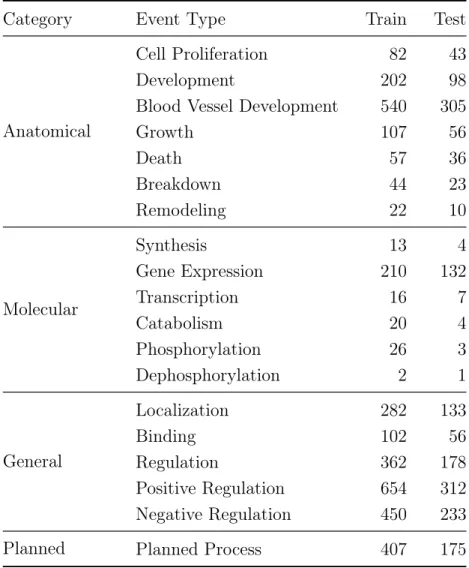
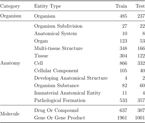
We use the MLEE dataset [18] for this task. It consists of 262 PubMed abstracts divided into train and test sets with 175 and 87 abstracts respectively. As this dataset is compiled for the task of event extraction, PubMed abstracts are annotated for event triggers, associated entities and role of the entities in an event. This dataset is limited to 19 types of events spanning four broad categories - Anatomical, Molecular, General and Planned. Table 3.1 shows the distribution of various event types in train and test splits. From the entity information annotated in this dataset, we have 14 types of entities that can be associated with 19 event types. Table 3.2 highlights the various entity types present in the dataset.

Table 3.1: Distribution of Event Types

Category Event Type Train Test

Anatomical

Cell Proliferation 82 43

Development 202 98

Blood Vessel Development 540 305

Growth 107 56 Death 57 36 Breakdown 44 23 Remodeling 22 10 Molecular Synthesis 13 4 Gene Expression 210 132 Transcription 16 7 Catabolism 20 4 Phosphorylation 26 3 Dephosphorylation 2 1 General Localization 282 133 Binding 102 56 Regulation 362 178 Positive Regulation 654 312 Negative Regulation 450 233

Table 3.2: Distribution of Entity Types

Category Entity Type Train Test

Organism Organism 485 237 Anatomy Organism Subdivision 27 22 Anatomical System 10 8 Organ 123 53 Multi-tissue Structure 348 166 Tissue 304 122 Cell 866 332 Cellular Component 105 40

Developing Anatomical Structure 4 2

Organism Substance 82 60

Immaterial Anatomical Entity 11 4

Pathological Formation 533 357

Molecule Drug Or Compound 637 307

Gene Or Gene Product 1961 1001

Although events in general can be represented with a single or multi-word trigger, most of the events in this dataset are characterized by single word triggers and less than 3.0% constitute multi-word triggers. While constructing trigger candidates, we include only single word triggers and treat all multi-word triggers as false negatives. Candidate generation for multi-word triggers is expensive in terms of the number of candidate triggers as it includes all possible consecutive word sequences present in the dataset, which dramatically increases the search space for actual triggers. Also, this large increase in the number of candidates cannot be justified, given the relatively small number of the actual multi-word triggers present in the training data.

Chapter 4 Methods

Event trigger classification consists of two subtasks – trigger detection and trigger type prediction. Trigger detection deals with distinguishing triggers from non-triggers while trigger type prediction predicts the event types for the triggers identified in the first subtask. Instead of approaching these two subtasks individually, we combine them into one task by introducing an additional class for non-triggers. As a result of this modification, we now have a multi-class classification problem with 19 event types and one non-trigger type (which plays the role of trigger detection). Multi-class models can be constructed using two different approaches, namely, extension to binary and transformation to binary classification. In the former, binary classification algorithms are modified to predict more than two classes while in the latter, multi-class multi-classification task is decomposed into multiple binary multi-classification problems and predictions from all the classifiers are used to determine the class of an instance. We adopt the extension to binary classification approach as it avoids a situation where large number of negative instances dominate the final outcomes (as is the case with the second approach). Before discussing specifics of our model, we will present a few fundamental concepts that are essential to develop a better understanding of our architecture.

Neural networks, more specifically, recurrent neural networks (RNNs) and their variants form the core component of our model. RNNs [25] are a class of neural networks known for their ability to capture sequential information from the data. Vanilla RNNs were once a popular choice for several NLP tasks such as language modeling [25, 26, 27], machine translation [28, 29] and sequence labelling [30]. They are composed of basic units called cells that recur over different inputs in the se-quence to form a chain like structure. They process the input in a sequential manner, aggregating the past information and using it to inform the current processing step. This allows the RNNs to process variable length sequences which became their strong selling point in NLP tasks. However, it was observed that as the sequence gets longer, RNN’s information retaining ability decreases and they are unable to retain clues from the distant past which may be relevant for processing the future time steps. With longer sequences, they also suffer from vanishing/exploding gradients [31]. These is-sues led to the development of several variants of RNN, a popular one being LSTM. LSTMs [32] are capable of remembering long-term dependencies and are commonly used in place of vanilla RNNs. An LSTM cell consists of three gates which regulate

the flow of information within the network. The forget gate decides what elements of the past are not needed and can be forgotten, the input gate controls what infor-mation of the input should be updated to the cell state, and theoutput gate decides what portion of the cell state should be output at the current time step. LSTMs, feed forward networks [33, Chapter 4] and external features form the basic constituents of our model and they are combined in a unique fashion to arrive at the architecture described in Section 4.2.

4.1 Preprocessing

Since this task is concerned with classifying triggers in biomedical literature, the input is in the form of PubMed abstracts. Along with event type information, these abstracts are also annotated for the entities and their semantic types. We believe that entity types hold important clues to event classification and to leverage this relationship, we replace all the entities in the abstract by their corresponding semantic types (as annotated in the data). Next, we decompose the abstract into sentences and words by using sentence segmenter and word tokenizer respectively. Each tokenized word is considered to be a trigger candidate. By this definition, the number of trigger candidates are ten times more than the actual triggers as observed in the training data. In order to reduce the search space for triggers, we adopt a two stage filtering approach to reduce the non-triggers in the trigger candidate list. In the first stage we completely ignore stop words and entities (i.e., words in entity spans) and treat all other words as triggers candidates. The second stage uses the unified medical language system (UMLS [34]) to eliminate trivial, domain neutral non-triggers. Using UMLS semantic types, we retrieve type information for each candidate word in the vocabulary of our corpus. Based on the semantic type information of the actual triggers in the training set (obtained through API calls to NLM’s UMLS Metathesaurus server), we have identified 33 semantic types (shown in Table 4.1) as valid types.

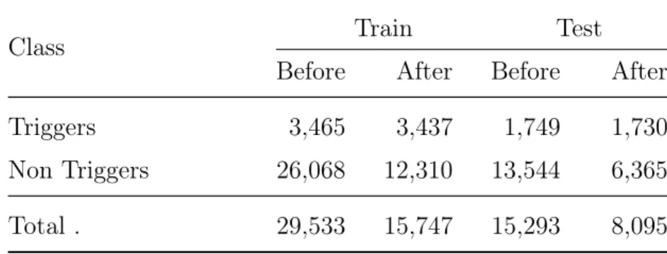
If a trigger candidate does not belong to at least one of these valid types, we remove the candidate from the trigger candidate list. The combined two stage filtering process reduces the non-triggers by 53.0% while loosing only 1.0% of the actual triggers as observed on the training data. Table 4.2 shows the actual numbers before and after the filtering process.

Table 4.1: Valid Semantic Types

Biologic Function Organism Function

Organ or Tissue Function Cell Function

Molecular Function Physiologic Function

Genetic Function Pathologic Function

Disease or Syndrome Cell or Molecular Dysfunction

Event Activity

Laboratory Procedure Diagnostic Procedure

Therapeutic or Preventive Procedure Research Activity Molecular Biology Research Technique Regulatory Activity

Phenomenon or Process Human-caused Phenomenon or Process

Natural Phenomenon or Process Functional Concept

Idea or Concept Temporal Concept

Qualitative Concept Quantitative Concept

Spatial Concept Chemical Viewed Functionally

Sign or Symptom Anatomical Abnormality

Neoplastic Process Social Behavior

Finding

Table 4.2: Data summary before and after candidate filtering process

Class Train Test

Before After Before After

Triggers 3,465 3,437 1,749 1,730

Non Triggers 26,068 12,310 13,544 6,365

Total . 29,533 15,747 15,293 8,095

4.2 Bidirectional LSTM with attention

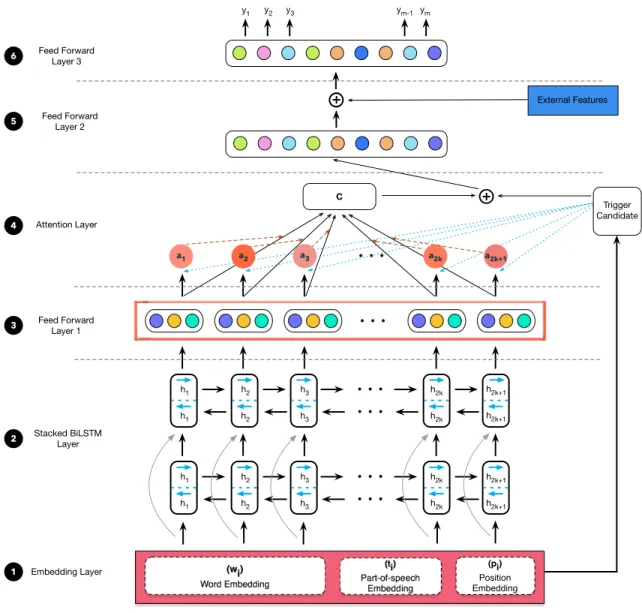
None of the existing architectures for biomedical trigger classification have explicitly considered the varying degree of influence of the words surrounding the trigger candi-date. We believe that differential treatment of contextual words is likely to improve the performance of the model. To test our hypothesis, we propose a novel architec-ture (shown in Figure 4.1) that uses an attention mechanism to learn the degree of importance of words in the context. It has six components: embedding layer, stacked bidirectional LSTM (BiLSTM) layer, attention layer and three feed forward layers.

h_2k+1 h_2k+1 h₁ h₁ h₂ h₂ h₃ h₃ h_2k h_2k h₁ h₁ h₂ h₂ h₃ h₃ h_2k h_2k h_2k+1 h_2k+1 a1 a2 a3 a2k a2k+1 External Features y₁ y₂ y₃ y_m-1 y_m C Stacked BiLSTM Layer Feed Forward Layer 1 Attention Layer Feed Forward Layer 2 Feed Forward Layer 3 (wi) Word Embedding (ti) Part-of-speech Embedding (pi) Position Embedding Embedding Layer Trigger Candidate 1 2 3 4 5 6

Figure 4.1: Event Trigger Classification Framework

4.2.1 Input embeddings

The input to neural network consists of two parts - X and q, whereX is the trigger

context and q is the trigger candidate. The trigger context is obtained from the

sentence containing the trigger candidate by using a window ofkwords to the left and

right of the trigger candidate. In other words, X = {xt k, ..., xt 1, xt, xt+1, ..., xt+k}, wherext±iarek words surrounding the trigger candidate on either side. Each word in the input is represented as e1 dimensional vector using word embedding table. Word

embeddings [35, 36] are pre-trained dense vectors that capture syntactic and semantic meaning of the word. Depending on whether xi is a word or entity type, the vector representation is obtained from either word embedding table or randomly initialized

type embeddings. Similarly, qis also mapped to its corresponding vector in the word

embedding table and it is used directly in layer 4 of Figure 4.1. Along with word

embeddings, we also use e2 dimensional part-of-speech (POS) and e3 dimensional

position embeddings for the trigger context. These embeddings are derived from randomly initialized weights which are updated during the model training process. These three embeddings are concatenated to form each input in sequence X, such

that X 2R(2k+1)⇥(e1+e2+e3). In other words, each _x

i is constructed as

xi =wi||ti||pi

where wi is the word embedding, ti and pi are POS and position embedding respec-tively and|| is the concatenation operator.

4.2.2 Stacked BiLSTM layer

The first component of the input pair – trigger context is passed through a two layered stacked BiLSTM. Essentially, each BiLSTM is composed of two LSTMs, one processing the input from left to right and the other processing the input from right to left. It generates two output vectors for each word and these vectors are concatenated with each other as shown in equations 4.1 – 4.3.

!

hi =Forward-LSTM(xi), (4.1)

hi =Backward-LSTM(xi), (4.2)

hi =!hi||hi, fori= 1, ...,2k+ 1 (4.3)

where !hi and hi are the output vectors of forward and backward LSTMs respec-tively and || is the concatenation operation. The output of first BiLSTM layer with d1 hidden units is concatenated with inputX before feeding it to the second BiLSTM

layer withd2hidden units. Each output, hifrom the second BiLSTM can be arranged in a matrix H such that H 2R(2k+1)⇥2d2. Next, the matrix_H is passed to a feed

for-ward network in layer 3 of Figure 4.1, which is composed ofl1densely interconnected

units called neurons. These neurons learn the mapping si = f(hiWi +bi), where bi is the bias unit, si is the output, Wi 2 R2d2⇥l1 is a learnable parameter of the net-work andf is a rectified linear unit (ReLU) function. Since we have 2k+ 1BiLSTM

outputs, we would need 2k+ 1 independent feed forward networks. The outputs of

all the feed forward networks can be represented as a matrix,S = [s1, s2, s3, ..., s2k+1]

4.2.3 Attention layer

In NLP, attention was first used in neural machine translation [37] where the decoder attends to different parts of the source sentence to generate the next target word. Recently, it has been applied to a variety of other NLP tasks such as textual entail-ment [38], question-answering [39] and text summarization [40]. Depending on the task at hand, a variety of attention strategies are available such as self attention, ad-ditive attention and multiplicative attention. Here, we use a multiplicative attention strategy inspired from Luong et al. [41], which involves using the trigger candidate to learn a weight matrix, Wa 2Re1⇥l1 and generating a weighted product for each word in the context. Mathematically, this translates to

a=sof tmax qWaST ,

c=aS

where a 2 R1⇥(2k+1) _{is the attention vector and c 2 R}1⇥l1 is the context vector.

The context vector is concatenated with the trigger candidate, q and fed to a feed

forward network (at layer 5) with l2 hidden units. The operations at this layer

are governed by h↵ = f [c||q]W↵ +b↵ , where b↵ is the bias unit, h↵ 2 R1⇥l2 and W↵ 2 R(l1+e1)⇥l2 are the output and weights of the feed forward network and f is a

ReLU function.

4.2.4 Feature Engineering

Besides the features learned by the neural network, we also provide explicitly engi-neered features to the final layer of the network. A brief description of these features are given below:

• For each instance, we obtain the part-of-speech (POS) tag of the trigger

candi-date and encode it as a r-dimensional one hot feature vector denoted as g1.

• As already discussed in Chapter 1, an event is described by the entities

asso-ciated with it. This suggests a correlation between the event and entity types which can be exploited by constructing a table, M 2 R(u+1)⇥v_{, where u = 14} is the number of entity types and v = 19 is the number of event types. The

extra row inM corresponds to “no-entity”, a situation where an event does not

have any entities as arguments. Table M is constructed using the entity-event

each input instance can be mapped onto a specific row in M by determining

the entity type that is closest to the trigger candidate in its three-hop depen-dency path. Thus, the feature vector for each instance is a v-dimensional row

vector denoted asg2.

• For each instance, we generate z-dimensional dependency encoding of the

can-didate trigger denoted asg3. We consider the dependency tags of those relations

in which the trigger candidate is either a governor or dependent.

The above features are concatenated with the previous output,h↵ and passed into

the final layer in Figure 4.1. Softmax activation function is applied over the outputs from the final layer to generate a probability distribution over the event types. The operations at the final layer is given by p=sof tmax Wo[g1||g2||g3||h↵] +bo , where

g1, g2, g3 are the three explicitly engineered feature vectors, Wo 2 R(r+v+z+l2)⇥20 is a learnable network parameter,bo is the bias unit andp2R20is a vector of probability estimates for the event types. Using back propagation [42], the weights of the different network components are updated recursively to minimize the classification errors. This involves minimizing the objective function

J(✓) = 1 n n X i=1 m X j=1 yijlogpij,

where ✓ is a learnable parameter of all the neural network components in our archi-tecture, n andm are the total numbers of training instances and classes respectively, yij is the ground truth and pij is the predicted probability of ith input belonging to

jth _{class. The magnitude of errors from the objective function determines the} mag-nitude of updates propagated back to the network. We use optimization technique to minimize the objective function by driving the weight updates in the direction of local or global minima.

Chapter 5 Experiments and Results

We conducted experiments using MLEE dataset to assess the performance of our model. The training data was divided into training set and validation set. The model was trained on the training set and fine tuned on validation set.

5.1 Experiments

After exploring several combination of hyperparameters such as hidden units, dropouts [43], initializations, embeddings and optimizers, we present below the experimental details that produced the best performance.

• Word Embeddings: We used 200 dimensional word embeddings published

by Pyysalo et al. [44]. The embeddings were trained on PubMed and PubMed Central (PMC) articles using word2vec model. The entity types did not have any pre-trained word embedding and hence, these were randomly initialized with truncated normal distribution with mean of 0.0 and standard deviation of 0.05

• Input Layer: The trigger context was constructed by setting the value of

k= 4. This yields a sequence of 9 words (four words each to the left and right

of the trigger candidate and the trigger candidate itself). We used sequence padding for instances going beyond sentence boundaries. Each word in the trigger context is encoded by 3 types of embeddings: e1 = 200 dimensional

word embedding concatenated with e2 = 30 dimensional POS embedding and

e3 = 20 dimensional position embedding to yield an input word vector of size

250.

• BiLSTM Layer: We used a two layer stacked BiLSTMs with d1 = d2 = 512

hidden units. The weights of each layer were initialized using truncated normal distribution with mean value of 0.0 and standard deviation of 0.05. A non-linear ReLU transformation was applied to the outputs of BiLSTM network. The dropout was set to 0.5 in both layers.

• Feed Forward Layers: These layers were initialized with truncated normal

distribution withl1 =l2 = 512hidden units. Similar to BiLSTMs, non-linearity

• Explicit features: We used 3 feature vectors at the final layer of our network.

The POS of the candidate trigger was encoded in a vector of size, r=6, the event type probabilities were encoded in a vector of size, v=19 and the dependency tags of trigger candidate were encoded in a vector of size, z=30. Combining these three features, we obtain a vector of size 55.

• Output layer: It consisted of 20 output units corresponding to 20 classes in

our task. We omit dropout at this layer and unlike the previous feed forward layers, we used softmax function to generate prediction probabilities.

• Model Training: The training data is split into 85% training set and 15%

validation set. We followed a batch gradient descent strategy with a batch size of 128. Adam [45] was used for optimization with a learning rate of 0.001. We trained the model on training set for 20 epochs. At the end of each epoch, we tested it on the validation set. The epoch that had the lowest validation loss was used to make predictions on the blind test set.

From the above details, the architectural design and experimental setup might appear too specific to this task. These choices were made after carefully tuning the hyperparameters on a validation set. The hyperparameters such as hidden units, dropouts and number of hidden layers were chosen by gradually increasing their respective values until no further improvements in performance were observed. Thus, after several permutations and combinations of the network components and their values, we arrived at the architecture shown in Figure 4.1

5.2 Results

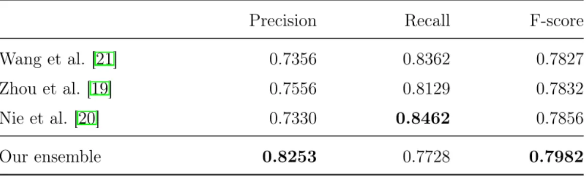
The performance of our model is evaluated using micro averaged measures of preci-sion, recall and F-score. While computing micro measures, we omit the non-trigger class as it is not an event type and it was added for convenience during the prepro-cessing step. We shall discuss the merits of our model by comparing it with some of the prior works as shown in Table 5.1. Nie et al. [20] achieve the best performance in this task. Hence, the performance improvements of our model are discussed with respect to their scores. Our best performing model is an ensemble of 50 models and it clocks an improvement of 1.3% (in F-score). Interestingly, it yields an improvement of 9.23% in precision while loosing 7.3% in recall. The benefits of ensembling and its various strategies are discussed in Section 5.2.1

Table 5.1: Comparison of our model against prior works

Precision Recall F-score

Wang et al. [21] 0.7356 0.8362 0.7827

Zhou et al. [19] 0.7556 0.8129 0.7832

Nie et al. [20] 0.7330 0.8462 0.7856

Our ensemble 0.8253 0.7728 0.7982

5.2.1 Model Ensembles

In any parametric learning approach, the final results vary across different runs even when the hyperparameters are kept constant. These variations are caused by random initializations of network weights resulting in different optimization paths leading to different local minima. Owing to the presence of multiple solutions, the error patterns and instances also vary across multiple runs. In order to reduce this vari-ability and improve the consistency of our results, we explore model ensembling [46] which essentially provides different strategies to combine predictions from multiple models creating a synergistic effect. Of the ensembling strategies [47] available, we use bagging approach with model averaging. In model averaging, we average the class probabilities of multiple models and class predictions are based on the averaged probabilities. We generate 50 ensembles by running ten models using different train-validation splits and choosing five best epochs in each model. Each train-train-validation split is created by randomly choosing 85% as train instance and the remaining 15% as validation instances. We made a conscious choice of retaining five best epochs from each model as we found that error patterns exhibited large variations around the vicinity of local minima.

5.2.2 Ablation Study

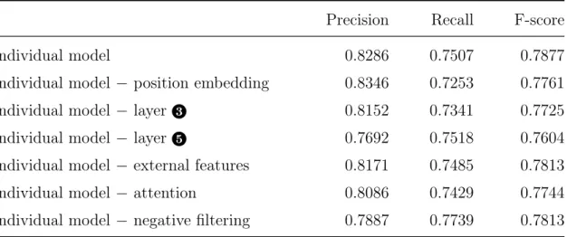
In this chapter, we saw the performance gains of our model against prior efforts. Now, we will try to understand the reasons behind these improvements. In ablation study, we remove the various components of the model to interpret the incremental gains in performance. This uncovers the contribution of individual components by comparing the model performance with and without the component. We have identified six such components for ablation experiments as shown in Table 5.2. In all the experiments, we have used individual model instead of the ensemble. Row 1 displays the score of

the individual model with all the components as shown in Figure 4.1. In rows 2 -7, “ ” operator indicates the removal of the component to its right. In row 3, the output of the LSTM is directly used by the attention layer bypassing the feed forward network at layer 3 in Figure 4.1. In row 4, we remove the feed forward network at

layer 5 of Figure 4.1 and directly pass the concatenated vectors along with external

features to layer 6.

Table 5.2: Component level performance analysis

Precision Recall F-score

Individual model 0.8286 0.7507 0.7877

Individual model position embedding 0.8346 0.7253 0.7761

Individual model layer 3 0.8152 0.7341 0.7725

Individual model layer 5 0.7692 0.7518 0.7604

Individual model external features 0.8171 0.7485 0.7813

Individual model attention 0.8086 0.7429 0.7744

Individual model negative filtering 0.7887 0.7739 0.7813

All the performance gains are measured with respect to the F-scores. In row 6, it can be seen that removal of the attention layer decreases the performance by 1.3%. This confirms our conjecture that the words in trigger context exert varying degree of influence on the trigger candidate and learning the degree of influence is imperative to the classification task. The benefit of adding feed forward networks at layers 3

and 5 of Figure 4.1 can be noticed through the performance improvement of 1.5% and

2.7% respectively. Even though position embeddings might seem trivial in this task, it contributes to a modest increase of 1.2%. Negative filtering generates an improvement of 0.6%, indicating a promising avenue for further exploration. Ensembling is also one of the contributors to the performance (refer Table 5.1), with an improvement of 1.0% over the individual model.

5.3 Analysis

On examining the instances where the model failed to predict the correct type, we found that a majority of the errors were due to actual triggers being classified as non-triggers or vice versa with very few inter-event type errors. More specifically, around 90.5% of the total errors were due to trigger/non-trigger type misclassification and the

remaining 9.5% were due to inter-event type errors. Here, we will focus our analysis on the former type of errors. Among these errors, false negatives (triggers being classified as non-trigger) were higher than false positives (non-triggers being classified as triggers). On further investigating each of these misclassified trigger candidates and their context, we discovered that these errors could be broadly grouped into two buckets as shown in Figure 5.1.

Sentence 1: Here, we expressed the catalytic domain of VEGFR-2 as a soluble active kinase using Bac-to-Bac expression system …

Sentence 2: … coculture of F-2 cells with A431 cells led to the formation of A431 cell nests constantly surrounded by tube-like networks consisting of F-2 cells.

Trigger candidate

(a) Bucket 1 errors

Sentence 3: … revealed that the effects of LeTx on tumor perfusion were remarkably rapid and resulted in a marked reduction of perfusion within the tumor …

Sentence 4: sDll4 similarly induced defective vascular response in tumor implants leading to reduced tumor growth.

- Trigger candidate - Event 1 - Event 2 Bold Italics (b) Bucket 2 errors Figure 5.1: Error patterns

The first bucket (Figure 5.1a) contains errors due to incorrect ground truth an-notation. For example, consider Sentence 1, the word “expressed” is used to describe the experiment performed on VEGFR-2 and it does not describe an entity/event regulating another entity/event. In Sentence 2, we notice that the word “formation” describes a “development” event. However, it was not annotated as a trigger word in the MLEE corpus. The second bucket (Figure 5.1b) corresponds to those candidates with complex event structure spanning across words/phrases far off from the trigger candidate. Sentence 3 is an example of nested events where the trigger word “resulted” interconnects two independent events, event 1 and event 2 (as shown in Figure 5.1b). Similarly, in Sentence 4, the trigger word “leading” interconnects an event on its left to another event on its right. These errors can be explained by revisiting the trig-ger context which is restricted to a window of k words on either side of the trigger

candidate. Nested events, more often extend beyond this context window and hence they are not available to our model. It would appear that the most obvious solution is to consider the entire sentence as the trigger context. However, when the entire sentence was used as the context, the model failed to capture the nuances in the im-mediate vicinity of the trigger candidate and it resulted in far more errors than using a context window approach. Therefore, exploring various strategies to acknowledge the presence of other events around the trigger candidate could potentially improve the performance.

Chapter 6 Reproducibility

There has been a growing concern over the reproducibility aspects of scientific re-search. In particular, this concern is more relevant to the fields of natural language processing, machine learning and deep learning where the number of system variables is large and only the right combination of these variables can reproduce the desired result. In order to facilitate reproducibility of our methods and allow the biomed-ical community to utilize and extend our system, we release all our project related files online1_{. In this chapter, we will discuss the finer details of implementing the}

system described in Chapter 4. This chapter contains references to various project related scripts and functions (available on github1_{) and it is advised to refer to these}

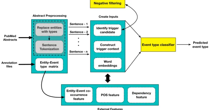
files to develop a better understanding of our system. From a software engineering perspective, the different modules of the system are laid out as shown in Figure 6.1.

Replace entities with types Entity-Event type matrix Sentence Tokenization Dependency feature POS feature Entity-Event co-occurrence feature Identify trigger candidate Negative filtering Construct trigger context Word embeddings

Event type classifier

Sentence - 1 Sentence - 2 Sentence - n Abstract Preprocessing External Features Create Inputs Predicted event type PubMed Abstracts Annotation files

Figure 6.1: System Architecture

Before we begin with the discussion, let us reiterate the goal of this task. Given a PubMed abstract, extract and classify the biomedical event triggers into their biomed-ical event types.

6.1 Abstract Preprocessing

The dataset consists of three types of files - the PubMed abstract, event annotation file and entity annotation file. The event annotation file provides the trigger spans, trigger words and event type information while the entity annotation file provides entity spans and entity type information. In this section, we discuss the classes and methods defined inpreprocess_abstracts.py that reads the abstract, replaces the enti-ties with their corresponding types and divides the abstract into individual sentences. The process_abstracts method iterates over each abstract and its corresponding an-notation files. It invokes the extract_triggers_entities function that extracts the location and type of the entities/trigger words from the annotation files. The loca-tion and entity type informaloca-tion are used by replace_entities function to locate the entities in the abstract and replace them with their corresponding entity types. The location and event type of the triggers are used to locate the triggers in the abstract and label them with their corresponding event types. This act of labeling the triggers becomes useful at the time of constructing the inputs, for generating the target class of triggers. Next, the abstract is passed to a sentence tokenizer, which uses regular expressions to determine the end of a sentence. Regular expressions are also used to get rid of non-alphanumerical tokens as they contribute to noise in the trigger classification task.

As we process the abstracts and their annotation files, we also collect information on the entity and event types co-occurring with each other. This information is aggregated across all the abstracts in the training set and is stored as a co-occurrence matrix. At a later stage, this matrix is used to construct one of the external feature vectors that encodes the likelihood of an entity type occurring with different event types.

6.2 Negative Filtering

Negative filtering helps in eliminating some straightforward non-triggers and reducing the size of the trigger candidate candidate space. We adopt two types of negative filtering - rule based filtering and domain based filtering. Domain based filtering leverages the semantic types in UMLS to determine if a trigger candidate is a non-trigger word. The UMLS REST API is used to extract the semantic types of the actual trigger words in the training set. Treating these semantic types asvalid types,

negative_filtering.pyscript is used to determine if the trigger candidate belongs to one of the valid types. The script consists of several functions that perform a sequence of

REST API calls to query the semantic type of each trigger candidate. As the UMLS semantic types are mapped to concept unique identifiers (CUI) and not directly to words, we useiterate_search function to retrieve the concept unique identifier (CUI) for the trigger candidate. The CUI is passed as input to iterate_cui function which returns the semantic type of the trigger candidate. If the semantic type matches with any of the valid types, it is retained as a valid candidate, otherwise it is excluded from the trigger candidate list.

6.3 External Features

Three types of external features are provided to the output layer of our classifica-tion system. These features vary from one trigger candidate to another and they are extracted from the sentence containing the trigger candidate. Each feature is represented as a vector and the Python code to generate these vectors can be found inexternal_features.py. The script is organized as two functions described below.

• dependency_pos_feature: This function extracts two linguistic features from

the sentence. The first one is known as the dependency feature, which cap-tures the syntactic relationship between the trigger candidate and other words in the sentence while the second feature captures the POS tag of the trigger candidate. Before extracting these features, we first construct the parse tree of the sentence using the Brown BLLIP parser. The parse tree is used to identify those relations where the trigger candidate participates either as a governor or dependent. These relations are encoded as a feature vector of 30 dimen-sions, each representing one of the 30 predefined dependency relations. This 30-dimensional vector forms the dependency feature of the trigger candidate. All elements of the feature vector are zero except for those which represent the dependency relation of the trigger candidate. For the second feature vector, we extract the part-of-speech information of the trigger candidate and encode it as a six-dimensional one hot vector, each representing one of the six POS tags.

• entity_event_mapping: This function leverages the entity type around the

trig-ger candidate to generate a feature vector that represents the likelihood of a particular entity type co-occurring with the event types. Here, the first step is to explore the dependency paths and identify the entity type closest to the trig-ger candidate. We construct all possible dependency paths that pass through the trigger candidate. These paths are truncated to include up to three

de-pendency hops. Next, we iterate over all the truncated paths to determine the entity type closest to trigger candidate. From the co-occurrence matrix con-structed in Section 6.1, we retrieve the row vector corresponding to the entity type closest to the trigger candidate.

6.4 Input Data

The input to the classifier consists of a trigger candidate and the context in which it appears. These two inputs are constructed with the help of functions defined in

construct_input.py file. Earlier in Section 6.1, we saw that the abstracts are converted into a list of sentences. Here, these sentences are passed through a word tokenizer that splits each sentence into its constituent words. Next, we utilize the negative filtering component to determine if a word should be considered as a valid trigger candidate. For all valid trigger candidates, we create their context by extracting four words to the left and four words to the right of trigger candidate. Part-of-speech tagger is used to extract the POS tags of all words in the context. We also store the position of each word with respect to the trigger candidate. Mathematically, the words in the context are represented by three vector embeddings - word embedding derived from the word itself, POS embedding derived from POS tags and position embedding derived from position indices. Since we replace the entities in the abstract by their types, some context words may also be entity types. The entity types have no predefined word embeddings and hence they are represented by vectors with random values drawn from a uniform distribution. Additionally, we use the external features component to obtain three feature vectors for every input instance. Finally, we represent the ground truth label for each valid candidate as a one hot vector of 20 dimensions, each representing one of the 20 classes. Depending on the class to which the input belongs, all elements of the vector are zero except one which has the value of one.

6.5 Classifier

The neural network components of the classifier are implemented using the functions defined in neural_network_model.py. A brief description of these functions are as follows.

• embedding_layer: This function takes a scalar input and maps it to a vector.

vectors respectively. These vectors are updated along with other parameters of the network.

• stacked_lstm_layer: This function creates two layered bi-directional LSTMs

with 512 hidden units per layer. The input to the first layer is a concatenation of word embeddings, POS embeddings and position embeddings while the input to the second layer includes the output from the first layer along with the initial embeddings.

• attention_layer: This functions reduce the dimension of the BiLSTM output

vectors (obtained from previous function) and uses the trigger candidate to attend to specific parts of the context words. The vectors from the previous function are passed to a feed forward network with 512 hidden units to obtain context word vectors of a smaller dimension. The trigger candidate attends to these newly created context word vectors to obtain the attention weights. The attention weights are applied to these context word vectors to obtain a single vectoral representation of the entire context.

• neural_network: This function organizes the components described above to

create the classifier shown in Figure 4.1.

• construct_model: The input vectors and their dimensions are defined in this

function. The position and part-of-speech embeddings are also created here by invoking theembedding_layer function. The type of optimizer and loss function to be used in the training process are also instantiated in this function.

6.6 Training

In this step, we divide the training instances into two parts - 85% training subset and 15% validation set. The inputs from the training subset are passed to our classifier in batches of 128 instances and the parameters of the network are updated once for every batch. When the model has seen all instances from the training subset, we say that the model has been trained for one epoch and the trained model is referred to as model snapshot. We continue training the model for 20 such epochs. At the end of each epoch, we evaluate the performance of the model snapshot using the validation set. The snapshot with the lowest validation error is used to classify the triggers in the test set. While working with model ensembles, instead of selecting the snapshot with lowest validation error, we select top five (out of 20) snapshots with

least validation errors. We train 10 such independent models by shuffling training and validation instances. By following this process, we obtain 50 model ensembles (5 best snapshots ⇥ 10 models). The source code for training the ensemble model can

be found intrain_model_ensemble.py

6.7 Testing

Once we have the models trained on the training subset, we use test_model.py to evaluate the performance of the classifier on unseen test samples. We provide these samples to the 50 trained models which yield 50 probability estimates of each sample belonging to 20 classes. We average these individual probability outcomes and predict the class that has the highest probability score for that particular test instance. In the

evaluate function, the predictions and ground truth labels are compared with each other to count the number of true positives, false positives and false negatives for each of the 19 event types. These counts are used in computing the final performance of the system which is given by micro-averaged precision, recall and F-score.

Chapter 7 Conclusion

In this thesis, we developed a predictive model to identify and classify the trigger words into biomedical event types. We explored deep neural network architectures and proposed an attention mechanism that learns to attribute varying degrees of importance to words in the context. We also saw the benefits of adding a minimal yet effective set of features at the final layer of the network. Domain based candidate filtering plays an important role in reducing non-triggers and its contribution to the overall performance cannot be overlooked. The novelty of our architecture lies in the way different components (attention layer, stacked BiLSTMs, feed forward layers) interact with each other to produce a competent model.

7.1 Limitations

Even though our model performs better than the existing methods in terms of F-score, it has the following limitations.

• Our model does not support the classification of multi-word triggers. We have

intentionally restricted it to classify triggers at the word level due to the lack of a sizable portion of phrase triggers of length >1.

• The results of our model highlight an opposite trend in precision-recall measure.

We gain 9.23% in precision and loose 7.3% in recall with a net gain of 2 points in the overall trade off. Because of the gain in precision and loss in recall, this system might appear as a product of a straightforward precision-recall trade off. A higher net gain would have been more convincing of the performance of our system.

• The idea of using fixed length context prevents the system from looking at clues

beyond the context window. This is especially true for nested events where the clues are interspersed far away from the trigger word.

7.2 Future Work

Some of the future research directions in the area of biomedical event trigger classi-fication are as follows

• Exploring distance supervision techniques to include more trigger words and

phrases is likely to improve the performance of the existing system. Extending our model to support multi-word triggers can be beneficial if it can be done without compromising a lot on precision.

• From the results, it is clear that our model produces a higher precision than

recall, reversing the existing precision-recall trend seen in prior methods that depend on feature engineering. Expanding on our manually engineered feature set and exploring a hybrid combination of conventional learning methods with our deep learning system could yield positive results.

• While analyzing errors, we noticed that the model failed on those test instances

where the entity clues were far apart from the trigger word. Instead of using fixed length context, forming a dynamic context guided by syntactic structure and domain level clues could help in reducing these errors.

• Our UMLS guided filtering mechanism is based on the individual word and

does not take into account the context in which it is used. Exploring mecha-nisms to consider the contextual meaning of the word while filtering the trigger candidates could eliminate far more non-triggers leading to fewer false positives.