Automatic Object Detection and Categorisation in Deep Astronomical Imaging Surveys Using Unsupervised Machine Learning

(1)

Automatic object detection and categorisation

in deep astronomical imaging surveys using

unsupervised machine learning

Author:

Alexander HOCKING

Supervised by:

Dr. Yi Sun PRIMARY& Dr. J. E. Geach PRIMARY Dr. Neil Davey SECONDARY

Centre for Computer Science and Informatics Research School of Computing

University of Hertfordshire

Submitted to the University of Hertfordshire in partial fulfilment of the requirements of the degree of Doctor of Philosophy.

(2)

I present an unsupervised machine learning technique that automatically segments and labels galaxies in astronomical imaging surveys using only pixel data. Distinct from previous unsu-pervised machine learning approaches used in astronomy the technique uses no pre-selection or pre-filtering of target galaxy type to identify galaxies that are similar. I demonstrate the tech-nique on theHubble Space Telescope (HST) Frontier Fields. By training the algorithm using galaxies from one field (Abell 2744) and applying the result to another (MACS0416.1-2403), I show how the algorithm can cleanly separate early and late type galaxies without any form of pre-directed training for what an ‘early’ or ‘late’ type galaxy is. I present the results of testing the technique for generalisation and to identify its optimal configuration. I then apply the technique to the HST Cosmic Assembly Near-infrared Deep Extragalactic Legacy Survey (CANDELS) fields, creating a catalogue of 60000 labelled galaxies, grouped by their similarity. I show how the automatically identified groups contain galaxies with similar morphological (and photomet-ric) type. I compare the catalogue to human-classifications from the Galaxy Zoo: CANDELS project. Although there is not a direct mapping, I demonstrate a good level of concordance be-tween them. I publicly release the catalogue and a corresponding visual catalogue and galaxy similarity search facility at www.galaxyml.uk. I show how the technique can be used to iden-tify rarer objects and present lensed galaxy candidates from the CANDELS imaging. Finally, I consider how the technique can be improved and applied to future surveys to identify transient objects.

(3)

Declaration

I declare that no part of this work is being submitted concurrently for another award of the University or any other awarding body or institution. This thesis contains a substantial body of work that has not previously been submitted successfully for an award of the University or any other awarding body or institution.

The following parts of this submission have been published previously and/or undertaken as part of a previous degree or research programme:

1. Chapter 3: Sections 3.3.2, 3.3.3 and 3.4.2.1 were previously published in Hocking et al.,

2018Monthly Notices of the Royal Astronomical Society, 473, 1108

2. Chapter 4: Section 4.5 was previously published in Hocking et al., Unsupervised Image Analysis and Galaxy Categorisation in Multi-Wavelength Hubble Space Telescope

Im-ages Proceedings of the European Conference on Machine Learning (ECML) Doctoral

Consortium2015,

3. Chapter 5: The content of this chapter was previously published in Hocking et al., Mining Hubble Space Telescope Images, Proceedings of the International Joint Conference on Neural Networks 2017 (IJCNN)

4. Chapter 6: This content of this chapter was previously published in Hocking et al., 2018

Monthly Notices of the Royal Astronomical Society, 473, 1108

Except where indicated otherwise in the submission, the submission is my own work and has not previously been submitted successfully for any award.

(4)

I never intended to do a PhD, but I’m glad I did. The research involved is possibly the purest expression of innovation there is and that’s what I call fun!

Before I started I wasn’t sure what project to do other than ‘something to do with machine learn-ing’. I was always interested in Astronomy but it was not something I was remotely thinking of at the time. I met with Yi Sun and Neil Davey, and at about the same time they were approached by Jim Geach about a machine learning astronomy project. The course was set. It is true to say that supervisors and project choice can make or break a PhD. But, I honestly couldn’t have been more fortunate here. The guidance from Jim, Yi and Neil has been brilliant. Thank you very much for the opportunity, your advice and your effort. I hope you guys enjoyed the journey as much as I did.

The camaraderie involved in research is immense. The fellow researchers you get to know along the way make the day to day experience of research really fun. I’ve made friends for life. So thank you to Ankur, Jean, Zaheed, Ed, Marco and Dimitris, it wouldn’t have been the same without you guys.

My Mum & Dad didn’t have the best scholastic experience! Dad left school at 15, and Mum at 16. It’s just how it was for them - they were expected to go out to work. Study and qualifications, let alone University, was what other people did. It would have been very easy for them to project those same expectations on to their four children. But they did not. For most of my life I was completely unaware of the ‘ruse’ they played on me that doing well at school and going to University was normal. Mum & Dad, thank you for doing what you did.

There is, however, one person to blame for all the shenanigans over the past few years and that is my wife Nancy. I had been presented with a choice. I had successfully interviewed for a safe, well paying position, which was a fine but fairly unexciting job. The alternative was the pursuit of an MSc by Research - the opportunity to work in a professional research environment. An experience that was unlikely to be available in the future. Choosing to quit my existing job and reject the new one, felt, at the time, like jumping out of an aeroplane without a parachute. It felt like a crazy decision. But it was time to choose between what was meaningful and what was safe and expedient. At the moment of (in)decision my Wife provided me with a swift push in the right direction. Nancy, thank you for pushing me out of the aeroplane and for your unwavering support since.

(5)

galax-ies are to the left. They are numbered ‘0’ to ‘6’ with ‘0’ being spherical and ‘6’ being very elliptical. The spiral galaxies are to the right. The letters ‘a’, ‘b’ and ‘c’ signify a combination of the central bulge size and the compactness of the spiral arms. The spiral galaxies are ordered into two distinct types, the top fork shows ordinary spiral galaxies, and the bottom fork shows spiral galaxies that have a central bar. The ‘S0’ galaxies are known as lenticular galaxies. The subtypes were added to the classification system by De Vaucouleurs (1959). Ir-regular galaxies ‘Irr’ have irIr-regular morphologies and are difficult to place in the diagram, but were positioned to the right of the sequence. Credit: Mortlock (2013) . . . 3 1.3 Ten S´ersic 1D profiles each with a different S´ersic index,n. . . 4 1.4 The modelling of the light profile of a galaxy and its components. The top left

image is the original grey scale image of a galaxy. Three galaxy components were fitted: the top central image is the model of the central bulge, the top right image is the model for the central bar, the bottom left image is the model of the disk, the bottom middle image is the total model image which is a combi-nation of the bulge, disk and bar models. The bottom right image shows the enhanced residual after the total model is subtracted from the original image. Credit: ESO/E. De Souza and D. Gadotti/BUlge Disk Decomposition Analysis tool (BUDDA). . . 6 1.5 An example of the application of Concentration (C), Asymmetry (A) and

Clumpi-ness (S) to measure the structure of a galaxy. The images to the left are the original galaxy. The middle column contains the 180 degree rotation (top) and the blurred version of the galaxy (middle), the two right-hand images are the residual images. The bottom image is shows example radii used to calculate Concentration. Credit: Based onConselice (2014) . . . 8 2.1 The first image at the top is a subsection of a FITS image file. The image was

taken using the ACS camera and the F435W filter over many orbits of Hubble. The F435W is a broad band filter centred around 435nm, which is near the shortest wavelength available to Hubble. The second image is also produced using many orbits of observations with the ACS camera, but this time using the F814W filter. The bottom image is a composite created by using the STIFF tool (Bertin, 2012) to combine the image data from F435, F606W and F814W representing the R, G and B channels. . . 29

(9)

List of Figures viii

2.2 This is an RGB composite image of the HSTFrontier Field Abell 2744 (9000×

13000). The red, green and blue channels correspond to the F814W, F606W and F435W bands. . . 32 2.3 This is a composite RGB image of the CANDELS data for GOODS-North. It

is a combination of data from observations using filters F160W, F814W and F606W. The STScI team combine theHSTobservations into a mosaic. The field is 158 arcmin2. The individual square observations (∼2.2arcmin2) can be seen, and where the image is green or blue showing the lack of coverage in all filters. 34 2.4 This is the decision tree used to guide citizen scientists through the

classifica-tion process for the CANDELS dataset. Each citizen scientist starts at quesclassifica-tion T00 (top). Each galaxy is classified multiple times and each classification is provided by a different person. The answers for each question are consolidated into weighted consensus classification. Credit: Galaxy Zoo & Simmons et al. (2016a) . . . 36 3.1 A visualisation of the Histogram of Oriented Gradients (HoG) feature descriptor.

On the left is an image of a galaxy and on the right is the visualisation of the HoG feature. The image is segregated into 12×12 pixel cells and within each of these cells a histogram with 8 radial bins is created. The image to the right shows the histograms in each cell with the orientations and magnitudes of each bin represented by short lines. The size of the vector output is the number of radial bins by the number of pixel cells in the image. . . 41 3.2 The RIFT feature descriptor. A patch is divided into concentric rings of equal

width and a gradient orientation histogram is computed within each ring. The orientation is measured relative to the direction pointing away from the cen-tre. This maintains rotation invariance. A typical configuration is four rings and eight histogram orientations resulting in a 32 dimensional feature descrip-tor. Three sample points in the normalised patch (left) map to three different locations in the descriptor (right).dis the distance from the centre, andθis the

direction of the gradient. The magnitude of the gradient is indicated by bright-ness of the histogram cell. Credit: Lazebnik et al. (2005) . . . 41 3.3 The spin intensity feature descriptor. This descriptor encodes the distribution

of image brightness in the region of a centre point. d is the distance from the centre point and i is the intensity value forming a two dimension histogram (right). Each row of the histogram represents a histogram of the intensity value at a distancedfrom the centre of the patch. Three example sample points from the image patch (left) map to three locations in the descriptor (right). A typical configuration is to use ten bins for distance and ten bins for intensity values, resulting in a one-hundred dimension vector. Credit: Lazebnik et al. (2005) . . 42 3.4 Power spectrum feature descriptor. The original image (patch) is shown (top

left): this is an image of a galaxy, the 2D discrete fourier transform is calculated and the result is shown (top right), the average of the power values of the pixels within seven annular bins (bottom left), finally the averages form a 1D represen-tation of the power (bottom right). This results in seven features (one for each annular bin) for this patch. . . 43

(10)

3.5 AKAZE Key point detection on aHST FITS grayscale image. The green points are the key points detected by AKAZE. The gradient changes in the image at the centre of galaxies were identified as key points. However, not all the galaxies were detected and there is usually only one key point per galaxy. It is possi-ble that this method could be developed for the identification of sources but it shows little promise for classifying or clustering galaxies into groups. Therefore scale-space key point detectors are unlikely to be useful when applied to survey images. It maybe that they are more useful for individual images of large galax-ies where enough detail is resolved for the key point detectors to identify galaxy components. . . 45 3.6 These four images show how the Growing Neural Gas (GNG) algorithm works

to map and approximate data. (a) shows the sample data. The images (b), (c) and (d) show the progress of the GNG algorithm as it discovers and learns the structure of the data. . . 48 3.7 Top left, top right and bottom left show the identified clusters using

agglomer-ative clustering on images of digits. Bottom right is a dendogram visualisation of the hierarchy identified by an agglomerative clustering process. Thex axis identifes the data points. Theyaxis represents the degree of similarity. The lines identify the clusters the data points belong to, and the length of the lines are a measure of similarity. The root node of the dendogram is at the top. Credit: the code for the top left, top right and bottom left linkage plots from scikit-learn.org 50 3.8 The algorithms were run on a set of high dimensional test data that consisted

of 2000 features, with 50 spatially separated clusters. Each scatter plot shows the two principle components of applying PCA to the test data and the cluster centres identified by the algorithms were projected into the PCA space so they could be added to the plot. The retained variances for the first two principle components are 1.07%, 1.06%. The percentages are so low as the data has 2000 dimensions. . . 55 3.9 Visualisation of the Power Spectrum feature applied to a section of Abell2744

of the Frontier Fields. Top left is the feature reduced to projected into 2D us-ing principle component analysis. And the bottom left is a 2D visualisations of the same data using the non-linear technique called t-SNE. We can see there is extensive non linear structure in the data. The PCA plot shows extreme outliers which happen to be the extremely bright areas within the central bulges of galax-ies. By applying the natural log we achieve a more standard PCA visualisation at the top right. The bottom right is the same data with the natural log applied visualised using the t-SNE. . . 59 4.1 A sub section of the image representing the model (left) and the thresholded

HST image (right) of the galaxy cluster Abell 2744. Blue colours in the pro-cessed image highlight the unsupervised clusters that represent star-forming re-gions in the spiral and lensed galaxies. Yellow colours correspond to the unsu-pervised clusters that represent passive elliptical galaxies and the central passive regions of spiral galaxies. . . 70 4.2 The processed image at the top displays the result of applying the model to new

HST image of galaxy cluster MACS0416. Processed image of the MACSJ0416 galaxy cluster. HST composite RGB image of the MACSJ0416 galaxy cluster. . 71

(11)

List of Figures x

5.1 This shows theHSTimage of MACSJ0416 in the F606W filter. The red circles represent detections listed in the official catalogue Merlin et al. (2016) and the green circles are the sources listed in the machine learning catalogue. . . 76 5.2 A detailed view of the sources identified in Frontier Field MACSJ0416. This

image is the F606W image from theHST. The red circles are the sources listed in the Merlin et al. (2016) catalogue and the green circles are the sources listed in the machine learning catalogue. This image is centred at 64.04925 (RA) and -24.0807 (Dec.) and is 4000×1900. . . 76 5.3 A detailed view of the sources identified in part of the COSMOS CANDELS

field. This is the F160W image from theHST. The red circles are the sources identified in the Skelton et al. (2014) catalogues and the green circles are the sources identified in the machine learning catalogue. This image is centred at 150.0971 (RA) and 2.31093 (Dec.), it is 3400×2800. . . 77 5.4 This is the segmentation map produced by the machine learning algorithm of

the same area as Figure 5.3. A group of pixels with the same colour marks the identification of an object. This shows the pixels considered to be single objects by the machine learning technique. . . 77 5.5 This shows the COSMOS galaxies from the official CANDELS catalogue that

did not appear in the machine learning catalogue. The half-light radius is the FLUX RADIUS parameter from Source Extractor. It is the circular aperture ra-dius enclosing half the total flux of the galaxy. The vast majority of the galaxies have a magnitude of 24 or higher suggesting that the threshold level used for source detection was too high for the machine learning technique to identify these objects. . . 78 5.6 Galaxies and point sources from the Hubble Space Telescope Frontier Fields

survey. Each column contains three examples of a object type starting on the left with elliptical/lenticulars, then spirals, background star-forming galaxies, lensed galaxies and finally point sources. The RGB channels are F435W, F606W and F814W. Images produced using data from: NASA and STScI . . . 81 5.7 The results from the applying the technique to sky area 1 are presented for

dif-ferent patch sizes of each feature for the purpose of late type and early type cut. 8 and 12 pixels square patches are the optimum for the pixel intensity power spectrum representation. The pixel intensity power spectrum and Spin Intensity features were tested on patches ranging from 8px×8px to 32px×32px patch sizes, RIFT was tested with patch sizes from 16px×16px to 40px×40px . . . 85 5.8 Two galaxies in the Frontier Field MACS0416. The green circles have diameters

of 8px (0.2400), the blue circles have diameters of 12px (0.3600) and the red circles have diameters of 16px (0.4800). These circles illustrate the sizes of overlapping patches. The images are 12.3600by 11.7900. . . 86 5.9 A chart of the effect of the number of GNG nodes, the GNG graph size, for

each of the representation types. Three different graph sizes were validated: 5000, 15000 and 25000 nodes. Pixel intensity power spectrum can produce good results even with a smaller GNG graph, however, the RIFT representation requires a larger graph size. . . 86 5.10 The performance of the similarity measure used when creating galaxy vector

representations. This plot shows the effect on the clustering performance when using the pixel intensity power spectrum representation. The Pearson correlation similarity measure consistently showed higher performance across all represen-tation types and applications. . . 88

(12)

5.11 The difference between using agglomerative clustering and K-means for clus-tering galaxies using different values of K, a pre-set parameter for the expected number of clusters. The pixel intensity power spectrum representation was most effective for identifying late type and early type galaxies. Agglomerative clus-tering consistently out-performed K-means for all representation types and ap-plications. . . 89 6.1 Examples of a sample of galaxies in MACS0416.1−2403 that the algorithm

au-tomatically identifies as being members of group ‘one’. Each image is 4.500×

4.500. The algorithm automatically identified this group and classified these galaxies using no data other than the image pixel intensity values from the F435W, F606W and F814W bands, and based classifications on the informa-tion in the Abell 2744 image. . . 95 6.2 Examples of a sample of galaxies in MACS0416.1−2403 that the algorithm

identifies as being members of group ‘two’. Each image measures 4.500×4.500 arcseconds. Lensed galaxies are included in this group. Again, the algorithm automatically identified this group and classified these galaxies using no data other than the image pixel intensity values from the F435W, F606W and F814W bands, and based classifications on the information in the Abell 2744 image. Note that in some cases the algorithm has correctly classified faint galaxies that are clearly in the stellar halo of an elliptical. . . 96 6.3 A colour-magnitude diagram of the galaxies in MACS0416.1−2403. The

galax-ies that the process identifgalax-ies as being members of group ‘one’ are labelled with the red triangles. The galaxies that the process identifies as members of group ‘two’ are labelled with blue circles. The process cleanly separates the early types in the red sequence and the late types in the blue cloud. . . 97 6.4 Histograms showing theM20morphological measure calculated for the galaxies

that the process identifies as being members of group one in red, and the galaxies that the process identifies as being in group two in blue. This appears to identify two populations of galaxies as found in Lotz et al. (2004). . . 97 6.5 These colour-colour diagrams show some of the classification groups in our

clas-sified CANDELS catalogue. The background grey points are a random sample of the entire population. In blue, red and black are galaxies from individual classifications. Many of the classifications appear as distinct clusters in colour-colour space. The top right shows galaxies from classification number 57 and one of its ‘child’ classifications number 86 which is an example of the hierarchy within the catalogue. The bottom left figure also shows the effect of the hierar-chy of classifications, level six being the most detailed classification level, and level one at the highest (coarsest) level. The bottom panels show different clas-sifications for point sources which track the stellar locus; note that in the bottom right panel I find different classifications for sources lying in the same colour space, indicating that, while colour information clearly enters into the classifi-cation, the algorithm can offer a more finely controlled object classification and selection. . . 102

(13)

List of Figures xii

6.6 These histograms show F606W total magnitudes obtained from the 3D-HST photometric catalogues of Skelton et al. (2014). They compare the magnitude distributions of galaxies given a specific classification (blue) with a random sam-ple of galaxies from the full entire population (grey). The vertical lines are the 5σ limiting magnitudes for the wide and deep CANDELS surveys. This figure

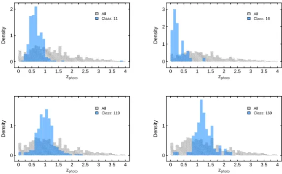
illustrates that the classification process groups galaxies into categories that can be easily described in terms of traditional descriptors such as magnitude, with distinct and ‘well behaved’ distributions. . . 103 6.7 I show the photometric redshifts of the galaxies for four different

classifica-tions identified by the machine learning technique. The photometric redshifts were obtained from Skelton et al. (2014) who determined them by using EAZY (Brammer et al., 2008). The histogram in grey shows the distribution for a ran-dom sample of the full population. As in Figure 6.6, each classification (based solely on pixel data) falls into well behaved distributions; for example, class 119 (bottom left) clearly contains galaxies atz≈1. Adding these ‘post-processed’ labels to automatically classified sources is useful in assigning astrophysical context to the groups the algorithm has identified. . . 104 6.8 Example images from the top level of three different CANDELS classification

groups (classification groups 7, 18 and 98). Each image is 600×600. The galaxies in each group are ordered row-wise in order of their similarity to the ‘average’ classification in the parameter space of the group. The top left image is the most similar galaxy to the ‘average’ and the bottom right is most dissimilar. The classification catalogue provides these as classification distances which can proxy as a quality flag. The distances are normalised between 0 and 1, with 0 being an identical match to the average. Here the RGB channels are the F160W, F814W and F606W bands, but note that the latter was not included in the learning.105 6.9 Examples of galaxies in three classification groups (30, 36, 48) from level one

(the coarsest classification) in the hierarchy. As before, each image is 600×600 and ordered left to right in order of similarity to the ‘average’ galaxy in the group. The RGB channels are the F160W, F814W and F606W bands. . . 106 6.10 Each row of 600×600images shows galaxies in an individual classification group,

and are selected from the lowest hierarchy level in that group. The galaxies are ordered left to right by their similarity to the average galaxy with the first panel most similar to the average. Again, the similarity of sources in each group is clear. The RGB channels are the F160W, F814W and F606W bands. . . 107 6.11 Examples of galaxies in two classification groups: group 8 at level one (low

level of refinement) and group 169 at level six (higher level of refinement). The images are 600×600and the RGB channels are the F160W, F814W and F606W bands. . . 108 6.12 The majority of the classifications groups are very clean. However, there are

some that are less so such as these three classification: 24, 41 and 56. Each row is an individual classification. The third row appears to include objects that are outliers distinct from other galaxy classifications. . . 108 6.13 Two potential strong lensing candidates (left and middle) and a known lens

(right). All three appear in the same classification group. The galaxy to the left is in UDS, ID16074 at location 02h17m06.s2(RA) and−05◦13017.006(Dec.). The galaxy in the middle is in EGS, ID10397 at 14h19m00.s12(RA) and+52◦42048.009(Dec.). The known strong lensing galaxy COSMOS 0013+2249 is shown on the right. . 109

(14)

6.14 This figure shows two examples of what I refer to as a ‘concordance’ group, where over 50% of the galaxies for which Galaxy Zoo classifications were made have a weighted fraction over 0.5 for question T00 A0 ‘is the target smooth

and rounded?’. The images show the top seven matches in the group and the

histograms compare the distribution of weighted fractions for questions T00 A0, A1 and A2 (see text) for galaxies in the group (blue histogram) compared to the full range of GZ classifications (grey histograms). Although not every machine learnt grouping can be described as a concordance group when compared to Galaxy Zoo classifications, this figure illustrates that the algorithm is creating groups that would have received a consistent human classification. . . 111 6.15 This figure shows two examples of what I refer to as a ‘concordance’ group,

where over 50% of the galaxies for which Galaxy Zoo classifications were made have a weighted fraction over 0.5 for question T00 A1 ‘does it contain features

or a disk?’. The images show the top seven matches in the group and the

his-tograms compare the distribution of weighted fractions for questions T00 A0, A1 and A2 (see text) for galaxies in the group (blue histogram) compared to the full range of GZ classifications (grey histograms). Although not every ma-chine learnt grouping can be described as a concordance group when compared to Galaxy Zoo classifications, this figure illustrates that the algorithm is creating groups that would have received a consistent human classification. . . 112 6.16 This figure shows two examples of what I refer to as a ‘concordance’ group,

where over 50% of the galaxies for which Galaxy Zoo classifications were made have a weighted fraction over 0.5 for question T00 A2 ‘is the target a star or

artifact?’. The images show the top seven matches in the group and the

his-tograms compare the distribution of weighted fractions for questions T00 A0, A1 and A2 (see text) for galaxies in the group (blue histogram) compared to the full range of GZ classifications (grey histograms). Although not every ma-chine learnt grouping can be described as a concordance group when compared to Galaxy Zoo classifications, this figure illustrates that the algorithm is creating groups that would have received a consistent human classification. . . 113 7.1 Autoencoded reconstructions. The top row contains original image patches and

the bottom row shows the reconstructions created by the convolutional autoen-coder. The reconstructions provide insight into how effectively the autoencoder has learnt the structure of the original image data. . . 119 A.1 The top left image is a toy image with zero values at every location except for

the vertical and horizontal lines with the value 1. The centre image is the output of applying the horizontal kernel. We can see the detection of the increase in gradient, the white vertical line, and the decrease in gradient, the black vertical line. The image to the top right shows the result of applying the vertical kernel. The three images in the bottom row show the effect on a real image of a rocket (left image). We can see that the vertical features are highlighted in the middle images, and the horizontal features are highlighted in the right images. . . 124 A.2 An example representation of the scale space of an image. The image at the

bottom is a standard grayscale image of a rocket. The images above it have an increasingly large Gaussian blur applied which removes detail until only the largest structures remain in the top image. . . 126

(15)

List of Figures xiv

A.3 The power spectrum of a time series. The power spectrum is symmetrical as can be seen in the right hand graphs. The zero frequency represents the average across the time series. For the power spectrum at the top the average is 10. The power spectrum shows a corresponding peak for the zero frequency. The lower two graphs show on the left test data consisting of two sine waves, one with a frequency of 2 and the second with a frequency of 8. Note that the average of the time series is 0. The corresponding power spectrum on the right shows the peaks at 2 and 8. The power spectrum is symmetrical. . . 128 A.4 When calculating a 2D power spectrum the frequency represents spatial

fre-quency or how the pixel intensities vary across the image. The ”DC term” cor-responding to zero frequency represents the average brightness across the image. 130 A.5 The images to the left have a sine wave with spatial frequency of 1 (top), 2

(middle) and 4 (bottom). The right three images show the corresponding 2D power spectra. The higher the spatial frequency the further from the central zero frequency. A smooth image has high power values in the centre, and edges or textures with large changes in pixel variation over short distances appear as larger values away from the centre. . . 131 A.6 The image to the top left contains a spatial frequency of three. The image to

the bottom left is the same image rotated 90◦. The top right image shows the 2D power spectrum of the top left image, and the bottom right image shows the 2D power spectrum of the bottom left image. This shows the effect on the 2D power spectrum of rotations. The power spectrum has the same 90◦rotation. . 132

(16)

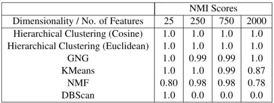
3.1 These are the results of running the algorithms on four test data sets. The data sets differed only in number of features: 25, 250, 750, and 2000 features. This is to test how well the algorithms perform on data with high numbers of di-mensions which is typical of image data. Each dataset contained 50 spatially separated, identically sized clusters created using random values from a Gaus-sian distribution with the same standard deviation. The performance measure used to identify how well the algorithms found the clusters is the normalised mutual information (NMI) score. A value of 1 shows the algorithm correctly identified the cluster membership of all data samples. . . 56 5.1 The list of galaxies classified by the astrophysicist in two sky areas. These are

used to evaluate the clusters produced by the unsupervised model and to test for generalisation. . . 83 5.2 The confusion matrix to show the effectiveness of categorising types of galaxy

in sky area 2. The clusters identified by the unsupervised method are compared to the classifications provided by an astrophysicist. This table shows the results for the pixel intensity power spectrum vector representation. We can see that the clusters effectively categorise spiral and elliptical galaxies, the lensed galax-ies were clustered together with background galaxgalax-ies. However, RIFT and Spin Intensity feature representations were more successful at distinguishing back-ground from lensed galaxies. . . 83 5.3 The results of identifying lensed galaxies in sky area 2 using three different

fea-ture representations. Rotation invariant feafea-ture transform was the most effective. . . . 84 5.4 The following preset-parameter options provided the best adjusted rand index

scores for the application of an early type (elliptical/lenticular) and late type (spirals/background/lensed) galaxy cut for each of the three chosen features. These results used the Pearson Correlation encoding, agglomerative clustering and 5000 GNG nodes to categorise the galaxies. The patch sizes were 8px×8px for PS, 16px×16px for Spin Intensity and 32px×32px for RIFT. . . 84 6.1 The format and columns of the catalogue produced by the machine learning

technique. . . 100 6.2 Fraction of top level machine learnt (ML) classification groups containing 50%

and 100% of the galaxies in the various Galaxy Zoo ‘clean’ classes. . . 111

(17)

Chapter 1

Introduction

Astronomers seek to understand the physical processes occurring within galaxies and how they evolve over cosmic time. A fundamental method astronomers apply to achieve this is the anal-ysis of images. By studying images in different bands of the electromagnetic spectrum, as-tronomers can analyse galaxies of different types, ages and masses, how they interact and merge, their structure and composition and how nearby galaxies differ from distant galaxies. In this Chapter I will provide a brief review of existing techniques used in Astronomy related to my research. I shall identify my research question in Section 1.3.

1.1 An overview of image analysis in astronomy

1.1.1 Classification systems

In the 1920s, using the largest telescope of the time, the Hooker 100-inch reflector, Edwin Hubble classified galaxies into two main morphological types, spirals and ellipticals (Hubble, 1926). He also identified a third type called an irregular galaxy. Figure 1.1 shows individual examples of a spiral and elliptical galaxy.

Hubble developed this scheme further to produce what is known as the Hubble Tuning Fork or Hubble Sequence (Hubble, 1936). Figure 1.2 shows a modern version of the Hubble Sequence. The term “Tuning Fork” is a reference to the split of spiral galaxies into two groups: with and without a central bar. The sequence gives the impression of evolution, although there was no

(18)

FIGURE 1.1: The elliptical galaxy M89 which is spheroid and spiral galaxy M101 known as the Pinwheel galaxy. Images taken by the Sloan Digital Sky Survey (SDSS) in bands r, g and i

Baillard et al. (2011)

evidence to support this. Astronomers were simply able to classify galaxies in the local Universe using this system. Sandage (2005) describes the development of this classification scheme. The original Hubble morphological scheme was developed using a series of photographic plates taken at the Mount Wilson Observatory (Hubble, 1926, 1936). De Vaucouleurs (1959, 1964) extended the original Hubble classification system to include further sub types, including a smooth transition beyond types Sc and SBc to the Irregulars. He introduced nomenclature to describe spirals without bars (SA) and intermediate types with weak bars (SAB), galaxies with rings (r), without rings (s) and intermediates (rs), as well as further classifications relating to the spiral arms, e.g. Sd (diffuse, broken arms with a faint central bulge), Im (highly irregular) and Sm (irregular with no bulge), effectively replacing Hubbles Irr classification. Holmberg (1958) also introduced plus and minus symbols to denote even finer divisions. In van den Bergh (1960a,b) added the concept of ‘order’ in the spiral arms, adding the labels I, I-II, II etc. to indicate increasing disorder within a Hubble type. These classifications also indicate increasing luminosity and the modern system covers a magnitude range of four between I and V (Sandage, 2005). More recently, detailed morphological features such as clumpiness and tidal tails are being classified by Galaxy Zoo (see Section 1.2.1).

More recent observations have imaged galaxies of higher cosmological redshift. Cosmological redshift arises as a consequence of photons of light travelling through an expanding Universe. The wavelength of the photons expands in direct proportion to the expansion of the Universe they travel through resulting in redshiftzdefined in equation 1.1, whereλ is wavelength.

(19)

Chapter 1.Introduction 3

FIGURE 1.2: The Hubble Tuning Fork morphological classification scheme. Elliptical galax-ies are to the left. They are numbered ‘0’ to ‘6’ with ‘0’ being spherical and ‘6’ being very elliptical. The spiral galaxies are to the right. The letters ‘a’, ‘b’ and ‘c’ signify a combination of the central bulge size and the compactness of the spiral arms. The spiral galaxies are ordered into two distinct types, the top fork shows ordinary spiral galaxies, and the bottom fork shows spiral galaxies that have a central bar. The ‘S0’ galaxies are known as lenticular galaxies. The subtypes were added to the classification system by De Vaucouleurs (1959). Irregular galaxies ‘Irr’ have irregular morphologies and are difficult to place in the diagram, but were positioned

to the right of the sequence. Credit: Mortlock (2013)

z+1=λobserved

λemitted

(1.1)

We cannot directly measure distance nor age directly, and therefore we use the measurable cosmological redshift as a proxy (Shu, 1982). Galaxies of high redshift appear as they did at a remote time when the Universe was much smaller than it is now. These galaxies are typically at an earlier stage of evolution and recent observations indicate that they cannot be classified as a single Hubble type and a new classification scheme may be required (Mortlock et al., 2013; Conselice, 2014).

1.1.2 Quantitative measures

1.1.2.1 Quantifying the light-profile of galaxies

The Hubble morphological classifications of galaxies are primarily a descriptive taxonomy dis-tinguishing particular galaxy types. Quantitive measures to analyse, categorise and classify individual galaxies in images have also developed. De Vaucouleurs’ law was one of the first models of how the surface brightness of an elliptical galaxy varies as a function of distance

(20)

log Radius

log Surface Brightness

n=1

n=10

FIGURE1.3: Ten S´ersic 1D profiles each with a different S´ersic index,n.

from its centre (de Vaucouleurs, 1948). De Vaucouleurs also noted that the disk component of many galaxies could be described by an exponential model (de Vaucouleurs, 1948; Freeman, 1970). Sérsic developed a more general form of the De Vaucouleurs’ law called the Sérsic pro-file (Sérsic, 1968). This is described in equation (1.2) whereI(r)is the intensity of a galaxy as a function of projected radiusrfrom its centre, I₀is the light intensity atr=0,α is the scale

length corresponding to the radius where the intensity drops by 1_e. The parameternis known as the S´ersic index and describes the profile shape, for example, usingn=4 reproduces de Vau-couleurs’ law andn=1 reproduces the exponential model. Figure 1.3 shows the S´ersic profiles forn=1 ton=10.

I(r) =I₀exp − r

α

!1/n!

(1.2)

These parametric models have been used extensively to perform structural studies of the 1d and 2d light profiles of galaxies. There has been a significant amount of work fitting S´ersic profiles to the profiles of nearby galaxies (Caon et al., 1993; Kormendy et al., 2009; Graham, 2013). A common approach is to model a galaxy’s central bulge and disk separately, known as

(21)

bulge/disk decomposition (Kormendy, 1977; Caon et al., 1993). Figure 1.4 shows an example of a bulge/disk decomposition. Three model profiles are fitted, representing the disk, central bulge and bar. Subtracting these from the original image creates a ‘residual’ which reveals how well the functions model these components of the galaxy and also highlight features such as dust lanes. More recently it was discovered that galaxy components may not have the same centre, for example, the existence of offset disks and bars (Kruk et al., 2017).

This approach has limitations due to assumptions such as that galaxies only have a single centre, and the ellipticity and angle of each component do not change with increasing distance from the galactic centre (Conselice, 2014). Also, many galaxies exhibit more than two components and so the decision of which galaxy components to fit requires visual inspection. The extensive morphological catalogues produced by Galaxy Zoo can be used here to automatically choose which components to fit (Willett et al., 2013, 2016; Simmons et al., 2016a). However, evaluating the residual image is a manual effort. Fitting the light profile of galaxies and their components is easier for small samples of nearby galaxies where it is possible to use an interactive fitting process. Tools have been developed to automate this process further (H¨außler et al., 2013). Kruk et al. (2018) successfully combined Galaxy Zoo morphological data and GALFITM, enhanced as part of the MegaMorph project (H¨außler et al., 2013), to study secular evolution of barred galaxies.

1.1.2.2 Quantifying the structure of galaxies

Perhaps the most popular methods of quantifying structure are the combination of concentration (C), asymmetry (A) and clumpiness (S) commonly known as the CAS system (Conselice, 2003); the Gini, and M20 measures (Lotz et al., 2004) and more recent measures by Freeman et al. (2013). These capture major features of galaxies, such as symmetry and clumpiness, without the need to make the sort of assumptions required by parametric light profile fitting methods such as the S´ersic profile. I briefly review the CAS parameters to provide an idea of the concept behind these techniques. I give a brief overview of Conselice (2014) and Figure 1.5 provides a visual illustration of applying CAS to a galaxy:

• Concentration (C) – a measure of the radial distribution of flux. One simple method for calculatingC, defined by Kent (1985) is to use the ratio of two radii containing, for

(22)

FIGURE 1.4: The modelling of the light profile of a galaxy and its components. The top left image is the original grey scale image of a galaxy. Three galaxy components were fitted: the top central image is the model of the central bulge, the top right image is the model for the central bar, the bottom left image is the model of the disk, the bottom middle image is the total model image which is a combination of the bulge, disk and bar models. The bottom right image shows the enhanced residual after the total model is subtracted from the original image. Credit:

ESO/E. De Souza and D. Gadotti/BUlge Disk Decomposition Analysis tool (BUDDA).

example, 20% (rinner) and 80% (router) of the total galaxy flux.

C=5×log₁₀

r_outer

rinner

(1.3)

• Asymmetry (A) – A galaxy imageI0is rotated 180 degrees around its centreI180and the pixel values are then subtracted from the original image.I0represents the pixel intensities of the original galaxy image andI180 represents the pixel intensities of the image after rotating it 180 degrees,B0 is a blank area of sky near the galaxy. Theminrefers to the global minimum found in an iterative process required to identify the centre of rotation. An initial guess is made and the left and right parts of the equation are calculated for this centre and for the eight surrounding points. The points that produce the minimum values are used to calculate the final value forA. Asymmetry is effective for distinguishing types of galaxies, for example, elliptical galaxies, being very symmetric haveA∼0.02±0.02 and late-type spiral (Sc-Sd) galaxies A∼0.17±0.1 (Conselice, 2014). The following

(23)

equation is given in Conselice (2014). The summations are applied to all of the pixel intensities in each 2D image matrix:I0,I180,B0,B180.

A=min ∑|I0−I180| ∑|I0| ! −min ∑|B0−B180| ∑|I0| ! (1.4)

• Clumpiness (S) – is calculated by subtracting a smoothed version of a galaxy from the original image. It is a measure of smoothness. Elliptical galaxies are smooth whereas star-forming regions in galaxies typically appear very clumpy. Ix,y is the original image,Bx,y

is the smoothed image and theσ smoothing kernel. The following is given in (Conselice,

2014). The summations apply to the pixel intensities within theIx,y,Ixσ,y,Bx,y,Bσx,yimages.

S=10× " ∑(Ix,y−Ixσ,y) ∑Ix,y ! − ∑(Bx,y−B σ x,y) ∑Ix,y !# (1.5)

Of great concern for any of these techniques is the ability to compare measurements when applying them to galaxies at different redshifts. To ensure comparable results an effective and common definition for the pixels that form a galaxy is required in any measurement. The most common choice when using CAS is the Petrosian radius (Petrosian, 1976; Conselice, 2014). The combination of CAS parameters and the Petrosian radius has been found to be effective when comparing over broad redshift ranges, whereas S´ersic profiles and other radius measures use assumptions or are affected by measurement effects such as surface brightness dimming, which render comparisons across redshift ranges very difficult Conselice (2014). The Petrosian radius, defined by the equation (1.6), is identified when the intensity at the radiusrpis equal to

the mean surface brightness withinrpmultiplied by a threshold valueη.

µ(rp) =η×µ(r<rp) (1.6)

Two further measures, in addition to CAS, are used to quantify galaxies are the Gini coefficient (Gini, 1912) andM20 (Lotz et al., 2004). These measures are sometimes used in combination with the CAS parameters, for example, in Lotz et al. (2008).

• The Gini coefficientG, as applied to astronomy (Abraham et al., 2003; Lotz et al., 2008), is based on the ordered cumulative distribution function of a galaxy’s pixel values. De-fined in Equation (1.7), whereXi is the pixel values, X is the mean pixel value, nis the

(24)

FIGURE1.5: An example of the application of Concentration (C), Asymmetry (A) and Clumpi-ness (S) to measure the structure of a galaxy. The images to the left are the original galaxy. The middle column contains the 180 degree rotation (top) and the blurred version of the galaxy (middle), the two right-hand images are the residual images. The bottom image is shows

ex-ample radii used to calculate Concentration. Credit: Based onConselice (2014)

number of pixels in the galaxy image (defined by the Petrosian radius). This coefficient represents the mean of the absolute difference between all pairwise combinations ofXi.

A coefficient value of 0 indicates a uniform galaxy profile and a value of 1 all the light is located in a single pixel.

G= 1 2X n(n−1) n

∑

i=1 n

∑

j=1

|

X

i

−

X

j

|

(1.7)

• M₂₀is defined as the normalized second order moment of the brightest 20% of the galaxy’s flux (W/m2), see equation (1.9). The Petrosian radius is typically used to define which pixels belong to the galaxy in the image.M₂₀is calculated by ordering the galaxy’s pixels by flux, sumMi over the brightest pixels until the sum is equal to 20% of the total flux

(25)

and then normalise withMtot to remove the dependency on total galaxy flux (or galaxy

size). The total second-order momentMtot (see equation 1.8) is the flux in each pixel fi

multiplied by the squared distance to the centre of the galaxy, summed over all the galaxy pixels. Where fiis the flux of a pixeliandxc,ycis the galaxy’s centre. The centre is found

by minimizingMtot. Mtot= n

∑

i=1 Mi= n

∑

i=1 fi·((xi−xc)2+ (yi−yc)2) (1.8) M20=log 10 ∑iMi Mtot ! while

_∑

i=1 fi<0.2ftot (1.9)

1.1.3 Combining features to identify properties and morphological types

Conselice (2003) discovered that the combination of CAS parameters formed a three dimen-sional parameter space that could be used to identify different morphological types of galaxy. For example, galaxies with a high light concentration, low asymmetry and low clumpiness are likely to be elliptical galaxies. Combinations of CAS values that could identify several other morphological types were established (Conselice, 2003).

Another useful combination of parameters was identified by Abraham et al. (2003). The Gini coefficient (Lotz et al., 2004), central concentration, and mean surface brightness, when sampled from nearby galaxies, were found to form a 3D-plane in parameter space.

Another example is the combination of parameters to form what astronomers call the fundamen-tal plane of elliptical galaxies (Sandage, 2005). The fundamenfundamen-tal plane is a relationship between the effective radius (the radius that contains half the total light of the galaxy), average surface brightness and central velocity dispersion (theσ of the radial velocities of the stellar population

in the interior of a galaxy) of normal elliptical galaxies. Any one of the three parameters may be estimated from the other two, as together they describe a plane that falls within the three dimensional parameter space.

All of these measures, with the exception of velocity dispersion, can be applied to images of galaxies to provide a quantitative measure of galaxies properties. They can be combined to form parameter spaces. Using the terminology of machine learning, these measures are an individual ‘feature’. The Fundamental Plane has three features, and CAS has three features. Together these features are combined to form a data manifold.

(26)

Although CAS, Gini and M20 have been popular, there are deficiencies. In particular, (Con-selice, 2003, 2014) published ranges of values for each of the CAS parameters for several morphological types. These values were measured in using specific data sets. However, the presented average values have large uncertainties leading to considerable overlap across mor-phological types. For example, the uncertainties for Irregular galaxies, edge-on disks and Ultra Luminous Infra-red Galaxies (ULIRGs) overlap significantly. It is also not clear why these values would remain consistent across observations from different telescopes or images of sig-nificantly different depths from the same telescope. The classifications are also limited to nearby objects.

Also, each of the CAS parameters reduces an individual galaxy to a single value based on a broad measure across the whole of the galaxy. Therefore, no consideration is made for different components within galaxies. The limitations of this method are perhaps not surprising con-sidering they were introduced in 2003, when computational resources were limited. It is now possible to analyse and create much more detailed models of galaxies. We are no longer limited to reducing an image of a galaxy to an ‘encoding’ of a few values such as the three CAS values. Instead, we can employ more complicated machine learning techniques such as Convolutional Neural Networks (see Section 1.2.3.1) and the model developed in this thesis. These machine learning models can encode the pixels of a galaxy into many more parameters allowing much more detailed information about galaxies to be retained and compared.

1.1.4 Surveys

There are two main types of imaging survey: images of a large region of sky, and images of several areas of sky that contain a known type of object. In this thesis the data I used considers both types.

Initial surveys performed in the early to mid 20th century were very limited when compared to the modern surveys of the last 30 years and those currently in development. Typically the numbers of galaxies used in research numbered in the hundreds or thousands (Djorgovski et al., 2013). There are now many more surveys and techniques that have been developed to image larger and larger areas of the sky. Perhaps the most famous large survey in visible light is the Sloan Digital Sky Survey (e.g. York et al., 2000; Stoughton et al., 2002; Abazajian et al., 2009; Blanton et al., 2017, SDSS). Using a 2.5-metre wide-field telescope the survey imaged over

(27)

10,000 deg2of the sky1. Its primary goal was to obtain images in five broad optical bands and obtain spectroscopy of over a million galaxies. The survey took ten years and the final data release (Abazajian et al., 2009), delivered in 2009, included almost a million galaxies and half a million stars.

Today, the SDSS is considered a large survey. But telescope and camera technology is improving very quickly. For example, in 2020, the space based Euclid telescope (Laureijs et al., 2011) will be launched. It is designed to observe 10 billion objects using optical (550 (green) to 920nm) and near-infrared (1000-2000nm) cameras.

Large, new ground-based telescopes are also arriving soon. The Large Synoptic Sky Telescope (Ivezic et al., 2014, LSST) will deliver perhaps the most ambitious optical survey of all. It will use a 3.2 gigapixel CCD camera to image 10,000 square degrees of the sky every three nights. The considerable survey area of 18,000 deg2will be imaged over 800 times in six optical bands (320nm to 1050nm). The telescope will image 20 billion galaxies and 20 billion stars, significantly more than previous surveys. One of the goals of the project is to ‘make a high-definition colour movie of the deep Universe’ (Ivezic et al., 2014). One of the most significant technical risks for the project is the availability of automated data analysis tools capable of processing the data quickly and accurately enough.

Although the LSST survey and Euclid will image billions of galaxies the vast majority of these galaxies will be too small or too dim for the telescopes to resolve morphological components. Therefore, morphological classification will only be possible for a subset of the total galaxies identified by these surveys.

1.2 Automated methods for analysing surveys

1.2.1 Galaxy Zoo: Crowd-sourcing visual classifications

The initial stages of most research into galaxy morphology has involved professional astronomers classifying hundreds to low thousands of galaxies. One of the largest manual efforts is a team of 65 astronomers who classified galaxies in the GOODS-South field of the Cosmic Assembly Near-infrared Dark Energy Legacy Survey (Kartaltepe et al., 2015, CANDELS).

(28)

To enable the visual classification process to be applied to much bigger datasets many more peo-ple are needed. This has led to the development of crowd-sourcing techniques and the Galaxy Zoo and Zooniverse projects (Lintott et al., 2008, 2010, GZ). GZ enables citizen scientists to participate in classifying surveys by using a website to classify galaxies sourced from surveys such as the SDSS and CANDELS. The citizen scientists, with typically limited knowledge of astronomy, are guided through the classification process using a decision tree of questions. Im-portantly, classification errors can be quantified as many classifications are obtained for each galaxy. GZ continues to classify huge numbers of galaxies from multiple surveys (Willett et al., 2013; Simmons et al., 2016a; Willett et al., 2016).

A key concern is ensuring consistent classification over time by individual citizen scientists and the weeding-out or down-weighting of classifications by unreliable classifiers (Simmons et al., 2016a).

A current development of the GZ and Zooniverse projects involves employing supervised ma-chine learning techniques (see Section 1.2.3) in combination with citizen scientist classifica-tions. An example of development in this direction is the combination of classifications from the Zooniverse Supernova Hunters project and a supervised machine learning algorithm to help identify supernovae in imaging from Pan-STARRS Survey for Transients Wright et al. (2017). Further development of these ideas focus on the optimum combination of citizen scientist and machine learning system in terms of classification accuracy and speed of classification (Beck et al., 2018).

1.2.2 Quantitative measures

Researchers have continued to develop tools and techniques to automate the analysis of surveys. In particular, tools to automate the calculation of structural parameters such as light profile mod-elling (see Figure 1.4) and non-parametric modmod-elling such as CAS and Gini/M20 (see Section 1.1.2.2 and equations 1.3, 1.7 and 1.9).

Prominent tools for profile fitting are GIM2D (Simard, 1998) and GALFIT (Peng et al., 2002). These tools perform automatic quantitative morphology analysis by decomposing all objects in an input image. An example of this process is seen in Figure 1.4 in Section 1.1.2.1. The method has been successfully applied to perform bulge/disk decompositions of the galaxies in the SDSS survey (Simard et al., 2011). The user specifies up front which functions (such as a

(29)

S´ersic profile, or an exponential) to fit to the light profile. Estimating the number of components is a trial and error process using chi-squared and visually inspecting the pattern of residuals to identify the best fit. However, for fitting simpler models such as for bulge disc decomposition, there is little or no human interaction allowing their use for automated survey analysis.

The Galapagos tool (Barden et al., 2012) is a data pipeline that automates the application of GALFIT for simpler decompositions. Van der Wel et al. (2012) used Galapagos to perform structural decompositions of the CANDELS survey (See Section 2.5).

Other examples are Megamorph (H¨außler et al., 2013), a project to extend GALFIT to fit models to multi-wavelength data. Also, PyMorph (Vikram et al., 2010) a tool to automate object location (source extraction), model fitting with GALFIT and the calculation of CAS and Gini/M20. Some tools employ image analysis techniques to identify and categorise individual galaxy com-ponents. Ganalyzer studies spiral structure (Shamir, 2011). This tool computes the slopes of the peaks detected in radial intensity plots to measure the spirality of a galaxy and determine its morphological class. The authors claim that this is a difficult manual task and in many cases the tool provides a more accurate analysis.

SpArcFiRe (Davis and Hayes, 2014) automatically identifies and categorises spiral arm seg-ments. It categorises arm segments by using a least squares fit to a logarithmic spiral arc. It has been run on over 600,000 galaxies in the SDSS that are larger than 40 pixels across. They found a very good correlation between the quantitative description of the spiral structure and Galaxy Zoo classifications. Hart et al. (2017) used SpArcFiRe in combination with Galaxy Zoo data to constrain the mechanisms of spiral arm formation.

Automated tools, such as Galapagos, now resemble full data pipelines that contain source ex-traction, masking, segmentation, and object categorisation.

The advantage of these tools is that they allow the fast analysis of a large dataset. Though, whether the automation of these tools provides more accurate results is questionable.

The automation of structural decomposition tools has proved to be difficult. The main issue is that choosing which structural models to fit is very difficult without apriori knowledge of which structural components a galaxy has. For example, Allen et al. (2006) performed bulge and disk decomposition of over 10,000 galaxies and found that although many bulge and disc model fits were successful, they also ’automatically generated a lot of rubbish’. Simard et al. (2011) applied automation to analyse over a million SDSS galaxies. They restricted the analysis

(30)

to a simple bulge and disk model fit and explained that using a more complicated model is not possible ’without compromising convergence and avoiding parameter degeneracies’.

Therefore, to ensure a good model fit, human inspection is still required in order to know which galaxy subcomponents are present before deciding which models to fit. Of great help here is the use of Galaxy Zoo catalogue data as it contains this structural information. For example (Kruk et al., 2017) looked for evidence of secular evolution in barred spirals by first using Galaxy Zoo data to identify a sample of SDSS galaxies with strong bars. However, even with this higher quality sample of galaxies, it was still necessary to inspect the galaxy image, model and residual to identify which model fit was relevant. Of the initial sample of 5282 barred galaxies, 3466 had meaningful model fits.

More flexible and accurate models that can automatically analyse more complicated galaxy mor-phology are needed. Machine learning applied to image data holds much promise for developing models with these characteristics.

1.2.3 Machine learning in astronomy

Machine learning started to appear as a bonafide field of academic research in the 1950s. A 1959 paper by Arthur Samuel of IBM (”Some studies in machine learning using the game of checkers”) is possibly one of the first pieces of published research to use this term (Samuel, 2000).

Today machine learning algorithms and techniques are becoming increasingly important for the efficient analysis of current and future astronomical surveys. As described in Section 1.1.4 future surveys will generate more data than is practical for humans to examine exhaustively. Moreover, existing techniques are limited in their capacity to represent galaxies when applied in an automated fashion, for example, detailed structural decomposition is still a manual effort (see Section 1.2.2).

For experiments such as the Large Synoptic Survey Telescope (Ivezic et al., 2014, LSST), it will be important to rapidly and automatically analyse streams of imaging data to identify interesting transient phenomena and to mine the imaging data for rare sources which may yield discoveries.

(31)

Machine learning has three broad categories: supervised, unsupervised and reinforcement learn-ing (Bishop, 2006). I will review the applications of supervised and unsupervised learnlearn-ing to astronomy.

Reinforcement learning (Sutton and Barto, 1998) is currently under-represented in astronomy. However, its use has gained much recent publicity for automatically learning to play simple Atari games and to beat the world’s best Go player (Mnih et al., 2015; Silver et al., 2016). The basic idea behind reinforcement learning is an agent will continually perform some form of action or actions and win a reward for performing the actions successfully. By repeatedly performing the actions typically many hundreds of thousands or millions of times the agent learns the parameter space of behaviours that maximise the reward. The analysis of astronomy survey data does not have an interactive component and it is not clear what type of reward could be defined. These are the likely reasons that reinforcement learning has not yet been applied to astronomy. Supervised and Unsupervised machine learning techniques are used extensively in astronomy. The main difference between these two types of algorithms is that supervised machine learning algorithms require a training dataset with a set of outcomes or target measurements. The training dataset is used to build a prediction model that can predict the target value for new unseen data (Hastie et al., 2009). Unsupervised machine learning uses data without labels. Instead, the task is to reveal the underlying structure of data and how it is organised. By modelling the underlying structure it is possible to analyse new data for similar structure. I now consider the application of supervised and unsupervised algorithms in astronomy.

1.2.3.1 Supervised techniques

Supervised machine learning is used successfully in astronomy for both mundane and complex tasks. For example, there has been a significant effort made to develop techniques to improve the estimation of photometric redshifts. A photometric redshift is an estimate of cosmological redshift z (see Section 1.1.1). The estimate is calculated by measuring the brightness of an object at different wavelengths and comparing to model galaxy templates. There are several examples of neural networks being applied to this problem using labelled datasets (Firth et al., 2003; Collister and Lahav, 2004; Ball et al., 2004; Cavuoti et al., 2012; Brescia et al., 2013). Bonfield et al. (2010) used Gaussian process regression (GP) to estimate redshifts and compared the results for small training sets. They found GP to be superior to the neural network approaches

(32)

used in the ANNz tool (Collister and Lahav, 2004). More recent results, in the field of machine learning, reveal that neural networks are sensitive to training set size and typically have much higher accuracy when trained with larger datasets (LeCun et al., 2015).

A variety of supervised machine learning algorithms have been used to automatically classify objects such as stars and galaxies of different types, for example, by using neural networks (Klusch and Napiwotzki, 1993; Nielsen and Odewahn, 1994; Lahav et al., 1995; Odewahn, 1995) and support vector machines (SVM) galSVM (Company et al., 2008; Huertas-Company et al., 2009, 2011).

The decision tree based technique of Random forests has been deployed quite frequently in astronomy, for example, in Breiman (2001). They were also found to be the most effective at identifying transient features in Pan-STARRS imaging (Wright et al., 2015). Here they are using pixel data and not survey catalogue data (comma delimited text files containing features of galaxies). Random forests were also used for the identification and classification of Galactic filamentary structures (Riccio et al., 2016), again using pixel data. Miller et al. (2015) used Random forests for the inference of stellar parameters using a training set of 9000 spectra for which stellar parameters were already known.

Wndcharm, a tool originally developed for use in biological image analysis, has been employed several times in astronomy (Orlov et al., 2008). It calculates over a thousand different features from images and then classifies test images into pre-defined classes. It uses the Fisher discrim-inant (Bishop, 2006), a supervised algorithm, to identify the features that result in the most accurate classification performance. Kuminski and Shamir (2016) used Wndcharm to classify

∼3,000,000 SDSS galaxies as spiral or elliptical.

Combining Galaxy Zoo classifications with supervised machine learning algorithms has be-come a more prominent research area (Banerji et al., 2010). In this case, a neural network, a multi-layer perceptron (MLP), classified galaxies into one of three classes: early types, spirals and point sources/artifacts. The training set consisted of features such as parameters based on colours and profile fitting, and a second dataset using features based on adaptive moments, and a combination of the two. More recently Wright et al. (2017) combines classifications from citizen scientists of the Zooniverse Supernova Hunters project with those from a Convolutional Neural Network (CNN) to identify supernovae (a transient, short-lived object) in data from Pan-STARRS1.

Automatic Object Detection and Categorisation in Deep Astronomical Imaging Surveys Using Unsupervised Machine Learning