BotChase: Graph-Based Bot Detection Using Machine Learning

(1)

BotChase: Graph-Based Bot Detection

Using Machine Learning

by

Abbas Abou Daya

A thesis

presented to the University of Waterloo in fulfillment of the

thesis requirement for the degree of Master of Mathematics

in

Computer Science

Waterloo, Ontario, Canada, 2019 © Abbas Abou Daya 2019

(2)

Author’s Declaration

This thesis consists of material all of which I authored or co-authored: see Statement of Contributions included in the thesis. This is a true copy of the thesis, including any required final revisions, as accepted by my examiners.

(3)

Statement of Contributions

Chapter 3 and Chapter 4 borrow content from two papers "A Graph-Based Machine Learn-ing Approach for Bot Detection" [11] and "BotChase: Graph-Based Bot Detection usLearn-ing Machine Learning" [12].

(4)

Abstract

Bot detection using machine learning (ML), with network flow-level features, has been ex-tensively studied in the literature. However, existing flow-based approaches typically incur a high computational overhead and do not completely capture the network communication patterns, which can expose additional aspects of malicious hosts. Recently, bot detection systems which leverage communication graph analysis using ML have gained traction to overcome these limitations. A graph-based approach is rather intuitive, as graphs are true representations of network communications. In this thesis, we propose BotChase, a two-phased graph-based bot detection system that leverages both unsupervised and supervised ML. The first phase prunes presumable benign hosts, while the second phase achieves bot detection with high precision. Our prototype implementation of BotChase detects mul-tiple types of bots and exhibits robustness to zero-day attacks. It also accommodates different network topologies and is suitable for large-scale data. Compared to the state-of-the-art, BotChase outperforms an end-to-end system that employs flow-based features and performs particularly well in an online setting.

(5)

Acknowledgements

My genuine acknowledgements reach out to the ones who truly enabled me to be what I am today. I thank all the people who made this thesis possible.

(6)

Dedication

(7)

List of Figures

2.1 Intrusion kill-chain . . . 6

3.1 Components of the BotChase bot detection system . . . 12

3.2 Example topology of benign hosts with a gateway . . . 16

3.3 Example topology of benign hosts without a gateway . . . 16

3.4 Flowchart of node classification withi nodes and j features . . . 20

4.1 Comparison of SOM andk-Means with respect to training time . . . 28

4.2 Number of hosts outside the benign cluster (HOB) assigned by SOM with and without feature normalization . . . 32

4.3 Number of bots outside the benign cluster (BOB) assigned by SOM with and without feature normalization . . . 32

4.4 The variation of the training and testing time as time progresses . . . 44

(11)

List of Tables

4.1 Hardware Configuration of the Hadoop Cluster . . . 21

4.2 CTU-13 Dataset . . . 23

4.3 Graph Transform, Base Feature Extraction and Normalization Computation 23 4.4 Stand-alone Supervised Learning with F-Norm . . . 24

4.5 Stand-alone SL with F-Norm and Balanced Input . . . 25

4.6 Training Time of Stand-alone Supervised ML Classifiers . . . 25

4.7 Stand-alone Supervised Learning against Previously Unknown Bot . . . 26

4.8 k-Means Clustering with F-Norm . . . 27

4.9 SOM Clustering with F-Norm . . . 27

4.10 Supervised Learning with F-Norm . . . 29

4.11 Supervised Learning with F-Norm on the Balanced Dataset . . . 29

4.12 SOM with Newly Aggregated Dataset . . . 30

4.13 Training Time of Supervised Classifiers on the Pruned Dataset . . . 30

4.14 SOM Clustering without F-Norm . . . 31

4.15 Pearson’s Feature Correlation Matrix with F-Norm . . . 33

4.16 SOM Clustering without IDW and ODW . . . 33

4.17 Supervised Learning without IDW and ODW . . . 33

4.18 SOM Clustering without BC . . . 34

4.19 Supervised Learning without BC . . . 34

(12)

4.21 Supervised Learning with BotMiner Features without F-Norm . . . 36

4.22 Flow-Based Supervised Learning . . . 36

4.23 Supervised Learning with BClus Features and without F-Norm . . . 38

4.24 Supervised Learning with BClus Features and Modified F-Norm . . . 38

4.25 Supervised Learning with BClus Features and Two-way F-Norm . . . 38

4.26 Supervised Learning with F-Norm . . . 38

4.27 Supervised Learning with BClus Hybrid Features and F-Norm . . . 39

4.28 BClus End-to-End Results . . . 39

4.29 Accuracy of BotGM vs BotChase . . . 40

4.30 Ensemble Learning with Graph-Based Features . . . 41

4.31 Online Supervised Learning . . . 42

(13)

Chapter 1 Introduction

Undoubtedly, organizations are constantly under security threats, which not only cost bil-lions of dollars in damage and recovery, but also often detrimentally affect their reputation. A botnet-assisted attack is a widely known threat to these organizations. According to the U.S. Federal Bureau of Investigation, “Botnets caused over $9 billion in losses to U.S. vic-tims and over $110 billion globally. Approximately 500 million computers are infected each year, translating into 18 victims per second.” The most infamous attack, called Rustock, infected 1 million machines, sending up to 30 billion spam emails a day [22].

More recently, Mirai knocked offline 900,000 users of Deutsche Telekom [14]. Fur-thermore, an attack launched on Microsoft Windows systems, called WannaCry (or Wan-naCrypt), resulted in a widespread hijack of data from more than 230,000 computers in 150 countries [30]. Undeniably, in the face of a cyber arms race, attackers constantly find clever ways to sabotage networks via botnets, most importantly via zero-day attacks [20]. Hence, it is imperative to defend against these botnet-assisted attacks.

1.1 Botnets

A botnet is a collection of bots, agents in compromised hosts, controlled by botmasters via command and control (C2) channels. A malevolent adversary controls the bots through a botmaster, which could be distributed across several agents that reside within or outside the network. Hence, bots can be used for tasks ranging from distributed denial-of-service (DDoS), to massive-scale spamming, to fraud and identify theft. While bots thrive for different sinister purposes, they exhibit a similar behavioral pattern when studied up-close.

(14)

The intrusion kill-chain [41] dictates the general phases a malicious agent goes through in-order to reach and infest its target. To fend off these botnets, intrusion detection systems (IDS) were developed.

1.2 Intrusion Detection Systems

Devising an intrusion detection system for bot detection is an active area of research that can be broadly divided into two groups based on the employed detection method: signature-based and anomaly-based [45]. Signature-based methods detect pre-computed hashes of existing malware binaries. Signature-based IDSs can scale well and efficiently detect known threats. Systems using this method can be deployed as an agent running on an end host or a gateway, which can examine binaries in transfer on-the-fly. However, as they rely on a database of known threats, signature-based approaches require frequent database updates and can be easily subverted by unknown or modified attacks, such as zero-day attacks and polymorphism [27, 45]. This undermines their suitability for bot detection.

Anomaly-based methods are widely used in bot detection, which overcome the limi-tation of the signature-based approach [20, 26]. They first establish a baseline of normal behavior for the protected system and model a decision engine. The decision engine de-termines and alerts any divergence or statistical deviations from the norm as a threat. Machine learning (ML) is an ideal technique to automatically capture the normal behav-ior of a system. The use of ML has boosted the scalability and accuracy of anomaly-based IDSs [20,26].

1.3 Machine Learning

With an ascending advancement in technologies and deluge of flowing data, integrating AI into present day applications has become more of a necessity than a luxury. Aviation, autonomous transportation, drone navigation, sentient analysis and data mining are some of the renowned applications of current day AI research. However, it is not until recently that machine learning has become possible in fields which did not have the sufficient amount of data to have feasible predictive models.

For machine learning models and classifiers, there are a myriad of factors which de-termine their feasibility in production. Indicators such as false positives (FP) and false

(15)

negatives (FN) are critical to the success of a system in an inverse proportional manner. For example, it is not acceptable for an intrusion detection system to have machine learn-ing integrated with absurdly high FP and FN ratios [16]. Such systems are critical and very sensitive towards prediction outcomes. Allowing a bot to infiltrate a system as a FN would have immediate repercussions.

The most widely employed learning paradigms in ML include supervised and unsuper-vised. Supervised learning uses labeled training datasets to create models. It is employed to learn and identify patterns in the known training data. Typically, this approach is used to solve classification and regression problems. However, labeling is non-trivial and usually requires domain experts to manually label the datasets [20]. This is not only cumbersome but also error prone, even for small datasets. On the other hand, unsupervised learning uses unlabeled training datasets to create models that can discriminate between patterns in the data. This approach is most suited for clustering problems.

An important step prior to learning, or training an ML model, is feature extraction. These features act as discriminators for learning and inference, reduce data dimensionality, and increase the accuracy of ML models. The most commonly employed features in bot detection are flow-based (e.g., source and destination IPs, protocol, number of packets sent and/or received, etc.). However, these features do not capture the topological structure of the communication graph, which can expose additional aspects of malicious hosts. In addition, flow-level models can incur a high computational overhead, and can also be evaded by tweaking behavioral characteristics e.g., by changing packet structure [57].

Graph-basedfeatures, derived from flow-level information to reflect the true behaviour of hosts, are an alternate that overcome these limitations. We show that incorporating graph-based features into ML yields robustness against complex communication patterns and unknown attacks. Moreover, it allows for cross-network ML model training and inference.

1.4 Contributions

The major contributions of this thesis are as follows:

• We propose BotChase, an anomaly-based bot detection system which is protocol agnos-tic, robust to zero-day attacks, and suitable for large datasets.

• We show the limitations of stand-alone supervised learning. Therefore, we employ a two-phased ML approach that leverages both supervised and unsupervised learning. The first

(16)

phase filters presumable benign hosts. This is followed by a second phase on the pruned hosts, to achieve bot detection with high precision.

• We use graph-based features in BotChase and evaluate various ML techniques. The graph-based features, derived from network flows, overcome severe topological effects. These effects can skew bot behavior in different networks, exacerbating ML prediction. Furthermore, these features allow to combine data from different networks and promote spatial stability [43] in the models.

• We compare the performance of our graph-based features with flow-based features from BotMiner [37] and BClus [33] in a prototype implementation of BotChase. Furthermore, we compare BotChase with the end-to-end system proposed for BClus.

• We evaluate the BotChase prototype system in an online setting that recurrently trains and tests the ML models with new data. This is crucial to account for changes in network traffic patterns and host behavior.

1.5 Thesis Organization

The rest of the thesis is organized as follows. In Chapter 2, we present a background on the intrusion kill-chain and bot detection, highlight limitations of the state-of-the-art and motivate the problem. The system design of BotChase is delineated in Chapter 3. Then, we evaluate the prototype in Chapter 4. Finally, Chapter 5 concludes with a summary of our contributions and exposes future research directions.

(17)

Chapter 2 Background

In this section, we present an overview of the intrusion kill-chain, followed by the state-of-the-art in bot detection and highlight their limitations.

2.1 Intrusion Kill-Chain

Conventional bot detection assumes successful intrusions and focuses on individual events. However, in recent sophisticated botnets, a single adversary campaign consists of multiple small, less detectable attacks. Detecting these bots can be challenging, as a single campaign may develop over time with multiple steps, each designed to thwart a defense and take place in different timelines. To cope with this problem, a widely adopted network-based method is detection of C2 channels. C2 occurs at the early stages of a botnet’s lifecycle, thus its detection is essential to prevent malicious activities [35,54,62].

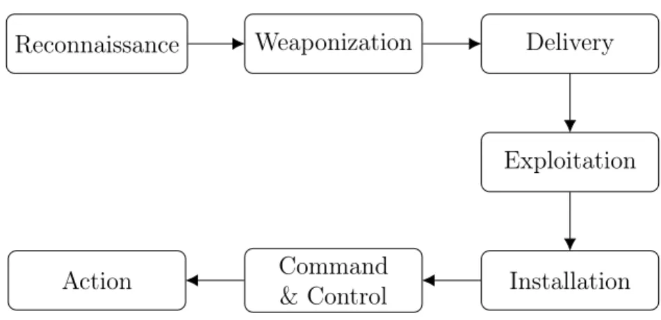
All adversarial attacks occurring in cyberspace have patterns that can be described as a chain of events—the intrusion kill-chain [41], depicted in Fig. 2.1. On a high-level, a bot starts with reconnaissance, observing and identifying a target in the network, and creating a weaponized payload. Weaponization of payloads take the form of malicious emails and attachments, which are delivered to the subject of interest. Exploitation starts after delivery, where the malevolent code gets triggered. While malicious code execution can be standalone, some malwares exploit applications on the subject’s machine. This can range from OS-based bugs (e.g., in RDP and PsExec) to application-based faults (e.g., in live processes, such as Google Chrome, Mozilla Firefox and Microsoft Word). The bot

(18)

Reconnaissance Weaponization Delivery Exploitation Installation Command & Control Action

Figure 2.1: Intrusion kill-chain

then proceeds with the installation of a security back-door on the system, which permits external persistent connections. These connections are then leveraged for C2.

On top of C2, the kill-chain identifies another crucial host-based bot behavior, lateral movement (LM). LM includes reconnaissance, credential stealing, and infiltrating other hosts controlled by bots to move laterally within the network to gain higher privileges and fulfill adversarial objectives. It is less likely that adversaries launch a successful intrusion without LM, as the adversarial target is typically not directly reachable from the outside of a network. Thus, detecting bot propagation using LM is also advantageous as it contributes to early botnet detection and classification [41, 45]. Nevertheless, both C2 and LM leave network footprints, which is the focus of our network-based bot detection mechanism.

2.2 Bot & Botnet Detection

Bot(net) detection has been an active area of research that has generated a substantial body of work. Common botnet detection approaches are passive. They assume successful intrusions and focus on identifying infected hosts (bots) or detecting C2 communications, by analyzing system logs and network data, using signature- or anomaly-based techniques.

2.2.1 Signature-Based

Signature-based techniques have commonly been used to detect pre-computed hashes of ex-isting malware in hosts and/or network traffic. They are also used to isolate internet relay

(19)

chat (IRC) based bots by detecting bot-like IRC nicknames [36], and to identify C2-related DNS requests by detecting C2-like domain names [53]. More generally, signature-based techniques have been employed to identify C2 by comparison with known C2 communi-cation patterns extracted from observed C2 traffic. It may also signify infected hosts by comparison with static profiles and behaviours of known bots [45]. Signature-based tech-niques owe their popularity to their ability to detect known threats in an efficient manner. However, they can be easily subverted by unknown or modified threats, such as zero-day at-tacks and polymorphism [27,45]. This undermines their suitability to detect sophisticated modern botnets.

2.2.2 Anomaly-Based

On the other hand, anomaly-based techniques use heuristics to associate certain behaviour and/or statistical features extracted from system or network logs, with bots and/or C2 traf-fic. C2 occurs at the early stages of a botnet’s lifecycle, thus its detection is deemed essential to prevent malicious activities. Most existing anomaly-based C2 detection techniques are based on the statistical features of packets and flows [19,23,36,37,44,48,49,54,56,58,60–62]. Works like [19, 44] are focused on specific communication protocols, such as IRC, provid-ing narrow-scoped solutions. On the other hand, Botminer [37] is a protocol-independent solution, which assumes that bots within the same botnet are characterized by similar ma-licious activities and communication patterns. This assumption is an over simplification, since botnets often randomize topologies [45] and communication patterns as we observe in newer malware, such as Mirai [14]. Other works, such as [54, 62], leverage ML and traffic-based statistical features for detecting C2 with low error rates. However, such tech-niques require that all flows are compared against each other to detect C2 traffic, which incurs a high computational overhead. In addition, they are unreliable, as they can be evaded with encryption and by tweaking flow characteristics [57]. Therefore, it is evident that a non-protocol-specific, more efficient, and less evadable detection method is desired. Based on the information used or the point of observation, anomaly-based detection can be classified ashost-based, network-based and hybrid.

(20)

2.3 Anomaly-Based Botnet Detection Scopes

2.3.1 Host-Based

Anomaly detection at the host level is useful in early botnet detection. Host-based anomaly detection systems enable quick microscopic per-host analysis, and are suited for known and observable malware activities. Host-based anomaly detection is typically accomplished by examining system traces, such as event logs or system calls. Existing works show that host-based anomaly detection has better potential compared to signature-host-based detection [26, 34, 35]. However, as they require extensive monitoring of system activities, they consume host system resources e.g., CPU cycles, memory, virtual machines. Consequently, they negatively impact user experience on the host.

Another downside of host-based anomaly detection is high error rates, since it experi-ences high false positives and false negatives when the established norm does not accurately represent the host behavior. Several studies, including [13] tend to resolve this problem by leveraging ML. However, though they indeed lower the error rates, their approaches are primarily designed for offline learning, requiring complete retraining of the ML model for each set of new input data. Since botnets rapidly evolve, it is imperative to leverage online, incremental learning to adapt the ML model to these changes.

2.3.2 Network-Based

Network-based anomaly detection collects and analyzes network traces, such as network packets and flow statistics. Detecting botnets by examining and monitoring network traf-fic has surfaced several times in the literature [37, 44, 54, 62]. Compared to host-based approaches, it offers a broader range of analysis, including traffic classification, botnet clustering, and network-wide anomaly detection with minimal to no performance degrada-tion of the monitored systems. Karasaridis et al. [44] propose an algorithm for detection and characterization of botnets based on the analysis of flow data in the transport layer. However, some existing works, including [44] are focused on specific network protocols, such as IRC and P2P, providing narrow-scoped solutions.

2.3.3 Hybrid

Existing works suggest that performing different types of botnet detection techniques in conjunction improves accuracy and precision [27]. Hybrid botnet detection collectively

(21)

applies host- and based techniques. EFFORT [55] integrates host- and network-based anomaly detection modules network-based on intrinsic characteristics of bots, and correlates detection results from them using ML. The evaluation shows that EFFORT detects mal-ware activities with low false positive (FP) and minimal performance overhead. However, the detection methods employed by EFFORT are mostly heuristics that assume certain bot behaviors varying in degree. This can be easily subverted by adversaries with prior knowledge about the intrusion detection system e.g., adversaries collaborating with insid-ers.

2.4 Graph-Based Approaches

Anomaly-based bot detection solutions that do not focus on detecting C2 per se, but rather identify bots by observing and analyzing their activities and behaviour, address some of the aforementioned issues. Graph-based approaches, where host network activities are represented by communication graphs, extracted from network flows and host-to-host communication patterns, are proposed in this regard [24, 25, 28, 31, 32, 38, 40, 42, 46, 50, 57, 59, 63, 64]. BotGM [46] builds host-to-host communication graphs from observed network flows, to capture communication patterns between hosts. A statistical technique, the inter-quartile method, is then used for outlier detection. Their results exhibit moderate accuracy with low false positives (FPs) based on different windowing parameters. However, BotGM generates multiple graphs for every single host. In other words, for every pair of unique IPs, a graph is constructed. Every node in the graph represents a unique 2-tuple of source and destination ports, with edges signifying the time sequence of communication. This entails a high overhead and will not scale for large datasets.

Chowdhury et al. [24] use ML for clustering the nodes in a graph, with a focus on dimensionality and topological characterization. Their assumption is that most benign hosts will be grouped in the same cluster due to similar connection patterns, hence can be eliminated from further analysis. Such a crucial reduction in nodes effectively minimizes detection overhead. However, their graph-based features are plagued by severe topological effects (cf., Chapter 4). They use statistical means and user-centric expert opinion to tag the remaining clusters as malicious or benign. Nevertheless, leveraging expert opinion can be cumbersome, error prone and infeasible for large datasets. Recently, rule-based host clustering and classification [63,64] have been proposed, where pre-defined thresholds are used to discriminate between benign and suspicious hosts. Unfortunately, relying on static thresholds makes the technique prone to evasion and less robust to ML-based outlier detection.

(22)

Graph-based approaches using ML for bot detection are intuitive and show promising results. In this thesis, we propose BotChase, an anomaly-, graph-based bot detection system, which is protocol agnostici.e., it detects bots regardless of the protocol. BotChase employs graph-based features in a two-phased ML approach, which is robust to zero-day attacks, spatially stable, and suitable for large datasets. It first employs unsupervised learning to reduce training data points for large datasets, followed by supervised learning to achieve bot detection with high precision.

(23)

Chapter 3 BotChase

3.1 Architecture

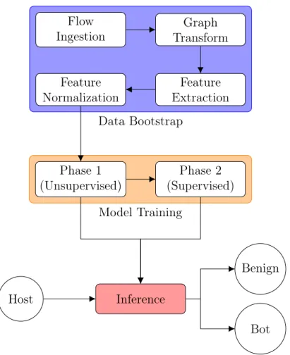
The BotChase system consists of three major components, as depicted in Fig. 3.1. These components pertain to data preparation and feature extraction, model training, and infer-ence. In the following, we discuss these components.

3.2 Dataset Bootstrap

3.2.1 Flow Ingestion

The input to the system are bidirectional network flows. These flows are transformed to form a set T that contains 4-tuple flows ti = {sipi, srcpktsi, dipi, dstpktsi}. Where

sipi is the source IP address that uniquely identifies a source host, srcpktsi quantifies the number of data packets sent by sipi to dipi, the destination host IP address. The number of destination packets, dstpktsi, is the number of data packets sent by dipi tosipi.

Set A is a set of tuples that have exclusive source and destination hosts. That is,

if multiple tuples have the same source and destination hosts, they are reduced to form an aggregated exclusive tuple ax ∈ A, such that ax = {sipx, srcpktsx, dipx, dstpktsx}. Therefore, if two tuples ti, tj ∈ T have the same source and destination hosts i.e., sipx =

(24)

Data Bootstrap

Model Training Flow

Ingestion TransformGraph Feature Extraction Feature

Normalization

Phase 1

(Unsupervised) (Supervised)Phase 2

Inference Host

Benign

Bot

Figure 3.1: Components of the BotChase bot detection system destination packets are aggregated in ax, such that

srcpktsx =

X

tk∈T |sipx=sipk,dipx=dipk

srcpktsk (3.1)

dstpktsx =

X

tk∈T | sipx=sipk,dipx=dipk

(25)

3.2.2 Graph Transform

The system creates a graph G(V, E), whereV is a set of nodes and E is a set of directed

edgesei,j from nodevi to nodevj with weight |ei,j|. The set of nodes V is a union of hosts from setA, such that

V = [

∀ax∈A

{sipx∪dipx}. (3.3)

For every ax ∈ A, there exist directed edges ei,j and ej,i from vi to vj and vj to vi, respectively, such thatsipx =vi and dipx =vj. Therefore,

E = [

∀ax∈A

{(sipx, dipx)∪(dipx, sipx)}. (3.4) The weights |ei,j| and |ej,i| of edges ei,j and ej,i are srcpktsx and dstpktsx, respectively. Moreover, if there exists a reverse tuple ay ∈ A | dipy = vi, sipy = vj, then |ei,j| =

srcpktsx + dstpktsy and |ej,i|=dstpktsx + srcpktsy.

3.2.3 Feature Extraction

BotChase creates the required graph-based feature set for the ML models. Features are intrinsic to the success of ML models that should genuinely represent and discriminate host behavior, especially that of bots. We leverage the following set of commonly used graph-based features.

• In-Degree (ID) and Out-Degree (OD)—The in-degree, fi,0, and out-degree, fi,1, of

a node vi ∈V are the number of its ingress and egress edges, respectively. F(ei,j) = ( 1, if ei,j ∈E 0, otherwise (3.5) fi,0 = X vj∈V, vi6=vj F(ej,i) ∀vi ∈V (3.6) fi,1 = X vj∈V, vi6=vj F(ei,j) ∀vi ∈V (3.7)

(26)

These features play an important role in the network behavior of a host. Although a higher ID for a host makes it a point of interest, it is often the case that nodes with a high ID offer a commonly demanded service. Therefore, observing ID alone may not signify malicious activity. For example, a gateway is a central point of communication in a network, but it is not necessarily a malicious endpoint. Intuitively, bots attempting to infect the network will tend to have a higher ID than benign hosts. Similarly, OD is also an intrinsic feature. Typically, in the reconnaissance stage of the intrusion kill-chain, bots attempt to survey the network. This mass surveillance can be captured via the OD.

• In-Degree Weight (IDW) and Out-Degree Weight (ODW)—These features

aug-ment the ID and OD of the nodes in the graph. The in-degree weight, fi,2, and the

out-degree weight,fi,3, of a nodevi ∈V is the sum of all the weights of its incoming and outgoing edges, respectively.

fi,2 = X vj∈V, vi6=vj, ej,i∈E |ej,i| ∀vi ∈V (3.8) fi,3 = X vj∈V, vi6=vj, ei,j∈E |ei,j| ∀vi ∈V (3.9) For a fine-grained differentiation, it is important to expose features that will eventually bring bots closer to each other, and discriminate bots from hosts. IDW and ODW features add another layer of information, further alienating the malicious hosts from the benign. Similar to ID, mass-data leeching bots will tend to expose a high IDW in the action phase of the intrusion kill-chain. Similarly, the ODW is the aggregate data packets a node has sent, which can potentially expose bots that mass-send payloads to hosts in a network.

• Betweenness Centrality (BC)—The betweenness centrality of a nodevi ∈V, inspired from social network analysis, is a measure of the number of shortest paths that pass through it, such that

fi,4 = X vj,vk∈V, vi6=vj6=vk σvjvk(vi) σvjvk ∀vi ∈V. (3.10)

Where σvjvk is the total number of shortest paths between node pairs vj, vk ∈ V, and

σvjvk(vi) is the number of shortest paths that pass through vi. This feature has a high

(27)

can alienate bots early on as they attempt their first connections. This is when the bots exhibit low IDW and ODW. Thus, it would be more favorable for the shortest paths in the network to pass through the host. Likewise, when the IDW and ODW increase, the BC of a node decreases immensely, as it is less favored for being included in shortest paths.

• Local Clustering Coefficient (LCC)—Unlike BC, local clustering coefficient has a

lower computational overhead, and it quantifies the neighborhood connectivity of a node

vi ∈V, such that fi,5 = P vj,vk∈Ni, vi=v6 j6=vkF(ej,k) |Ni|(|Ni| −1) ∀vi ∈V (3.11)

WhereNi is neighborhood set forvi, ∀vj ∈Ni |ei,j ∈E∨ej,i ∈E. The LCC feature can play an important role in discriminating malicious host’s behavior. Successfully infected hosts tend to exhibit a higher LCC, as bots often deploy collaborative P2P techniques, making adjacent host pairs strongly connected.

• Alpha Centrality (AC)—Alpha centrality, also inspired from social network analysis,

is a feature that generalizes the centrality of a nodevi ∈V. AC extends the Eigenvector centrality (EC), with the addition that nodes are also influenced by external sources. These external sources can be user-defined, according to their graphical analysis tech-nique. In EC, eachvi is assigned an influence scorexi, that is iteratively exchanged with adjacent nodes. In essence, EC is the relative weight of a node in the graph, such that connections to high-scoring nodes contribute more to the score ofvi. Hence, AC is given

as

fi,6 =αATi xi+ei ∀vi ∈V. (3.12) Where Ai is the adjacency matrix, ei is the external influence of node vi, and α is influence factor that controls the bias in between external and internal sources. AC is important for the intermediate and terminal phases of the intrusion kill-chain. Early on, it may be negligible. However, as time progresses and bots perform more actions in the network, their AC will gradually increase, making it discriminative.

3.2.4 Feature Normalization (F-Norm)

Topological alterations can severely affect the host’s behavior and pattern of communica-tion in the graph. For example, in Fig. 3.2,g acts as a gateway for hosth2to communicate

(28)

h1 h2 g h3

h4 h5

Figure 3.2: Example topology of benign hosts with a gateway

h1 h2 h3

h4 h5

Figure 3.3: Example topology of benign hosts without a gateway

an ID of 2. In contrast, Fig. 3.3 shows the topology without a gateway, whereh2 commu-nicates with other hosts in the network individually. This boosts the ID of host h2 to 4. To alleviate this adverse effect of different network topologies, we normalize the above base features to include neighborhood relativity. To control the overhead of computing these normalized features, the neighborhood set Ni forvi ∈V is restricted to a certain depth D. The mean of j features forvi across its neighborsvk∈Ni are computed. Each feature for

vi is then normalized by incorporating neighborhood relativity. Thus, features relative to their neighborhood mean is given as

µi,m= P vk∈Nifk,m |Ni| ∀vi ∈V, 0≤m≤j (3.13) fi,m = fi,m µi,m ∀vi ∈V, 0≤m ≤j. (3.14)

After normalizing the features (with D = 2) for h2 and h4 with gateway, their IDs change from 2 to 0.8 and 3 to 1.1, respectively. Without the gateway, their IDs change

(29)

make hosts of the same nature look similar, making the topological alterations less severe. Similarly, in situations where network data is recorded over varying time intervals, IDW and ODW tend to increase substantially with larger time intervals. By normalizing features, the effect of time also diminishes. Appendix B depicts a straightforward approach for implementing F-Norm.

3.3 Model Training

The model accepts graph-based features as input and learns to distinguish between mali-cious and benign hosts. Two learning phases in BotChase are explained below.

3.3.1 Phase 1

The first ML phase performs unsupervised learning (UL) to cluster the hosts. Generally, benign hosts exhibit similar behavior that can be gauged by the graph-based features. These hosts exhibit resembling patterns in data, such as sending (OD/ODW) and receiving (ID/IDW) similar number of packets [24]. Since BC, LCC and AC are directly affected by these traits, their influence can be similar for all benign hosts. Therefore, maximizing the size of the “singleton” benign cluster is crucial.

Not only does this phase act as a first filter for new hosts, but also significantly reduces the training data for the second phase. If a host is clustered into the benign cluster, then it is strictly benign. However, it is important to note that a malicious host can also be incorrectly clustered into a benign cluster, adversely affecting system performance. Therefore, although the system objective is to maximize the size of the benign cluster, it is essential to jointly minimize the number of bots that are co-located in this cluster.

Various UL techniques can be deployed in this phase. Some of these techniques include k-Means, Density-Based Spatial Clustering (DBScan) and Self-Organizing Map (SOM).

• k-Means—The k-Means clustering algorithm attempts to find an optimal

assign-ment of nodes to k pre-determined clusters, such that the sum of the pairwise

dis-tance from the cluster mean is minimized. k-Means is static, it results in the same

cluster composition for a given dataset across different runs of the algorithm, with the same number of clusters and iterations. Assume k is set to the cardinality of the

label set. Idealistically, there should be a clean assignment of hosts to corresponding clusters. However, in reality, some benign hosts exhibit an outlier behavior. For

(30)

example, network nodes which host webservers and public APIs will depict a huge amount of data and connections. Thus, ID, IDW, OD and ODW features will be affected. Therefore, depending on the characteristics of the dataset, altering k may

adversely affect clustering performance.

• Density-Based Spatial Clustering (DBScan)—Unlike k-Means, DBScan does

not require the parameter k, the pre-determined number of clusters. In contrast, it

computes the clusters and assignment of nodes according to a rigid set of density-based rules. DBScan requires a pair of parameters: (i) p, the minimum number

of points required to be assigned as core points, and (ii) e, the minimum distance

required to detect points as neighbors. DBScan classifies points as core, edge or noise, where core points must haveppoints in their neighborhood with a distance less than e. Otherwise, if the point is reachable via e distance from at least one of the core points, it is considered an edge. The remaining points are considered noise and are not clustered. In other words, points are not forcefully assigned to clusters as some points may just be noise. Therefore, DBScan is capable of detecting non-linearly separable clusters.

• Self-Organizing Map (SOM)—A SOM is a special purpose artificial neural

net-work that applies competitive learning instead of error-correction. It is frequently used for dimensionality reduction and clusters similar data. However, the notion of similarity in SOM is looser than that of k-Means and DBScan. In SOM, neurons are

“pushed” towards the data points for a certain number of iterations. SOM uses the best matching unit to determine the winner neuron and updates its weights accord-ingly. Furthermore, it also applies a learning radius that affects all the other neurons, when a close-by neuron is updated. The number of neurons also plays an important role in clustering. Higher number of neurons results in the dispersion of nodes away from a single cluster. Importantly, the same logic applies tok-Means, hence the

clas-sifier with the best assignment must be selected, according to the objectives outlined in this phase.

3.3.2 Phase 2

Phase 1 separates the dataset between nodes that are inside and outside the benign cluster. All the nodes, ideally small, that reside outside the benign cluster are used as input to Phase 2 for further classification. Optimally, all the bots should be outside the benign cluster, regardless of whether or not they are co-located in the same cluster. Depending

(31)

on the amount of hosts outside the benign cluster, the supervised learning (SL) classifiers used in this phase will exhibit different results.

The primary objective in this phase is to maximize recall. Recall is a measure of how many bots are recalled correctly i.e., do not go unnoticed. It is proportional to the number of true positives (TPs) and inversely proportional to that of false negatives (FNs). Various SL classifiers can be deployed in this phase to achieve this objective, such as logistic regression (LR), support vector machine (SVM), feed-forward neural network (FNN) and decision tree (DT).

• Logistic Regression (LR) and Support Vector Machine (SVM)—LR focuses on

binary classification of its input, based on a sigmoid function. Input features are coupled with corresponding weights and fed into the function. Once a threshold p is defined,

usually0.5for the logistic function, it establishes the differentiator between positive and

negative points. Unlike LR, SVM is a non-probabilistic model for classification. It is not restricted to linearly separable datasets. There are various methods of computing SVM, including the renowned gradient-descent algorithm.

• Feed-forward Neural Network (FNN)—FNNs are artificial neural networks that do

not contain any cyclic dependencies. For a given feed-forward network with multiple layers, a feature vector is dispersed into the input layer, fed to the hidden layer of the network, and then to its output layer. While the input layer is constrained by the number of features exposed, the hidden and output layers are not. Every neuron may rely on a separate activation function that shapes the output. Popular activation functions for FNNs include identity, sigmoid, ReLU and binary step, among others. FNNs and the previously mentioned SL techniques are online classifiers. An online classifier is capable of incremental learning, as the weights associated with the deployed perceptrons are not static. This makes FNNs an attractive candidate for production-grade deployment.

• Decision Tree (DT)—DTs rely heavily on Information Entropy (IE) and gain to

con-jure its conditional routing procedure. Generally, IE states how many bits are needed to represent certain stochastic information in the dataset. By using DT, information gain is maximized from the observed data and the taken path. After training a DT, newly observed data points can be predicted upon. However, unlike all the other classifiers, DTs are not online. That is, optimally retraining a DT must be done from scratch.

Recall the objective from Phase 1, i.e., minimize hosts outside the benign cluster (HOB), while maximizing bots outside the benign cluster (BOB). This results in a mini-mal training dataset for Phase 2. Also, it is expected that the resultant training dataset

(32)

from Phase 1 would be unbalanced, with a bias towards benign hosts. This may prove problematic for LR, SVM and FNN in achieving high recall rates.

3.4 Inference

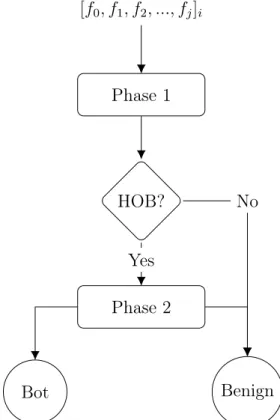
Once the models are trained, they are deployed in the system to perform bot detection. Ideally, the system must allow for two modes of execution: (i) model (re)training, to adjust to the dynamics of the network, and (ii) inference,i.e., for a given host predict whether or not it is a bot. In BotChase, the inference unfolds in two steps—presumable benign hosts get filtered out in Phase 1 as they get assigned to the benign cluster, while suspicious hosts assigned to a different cluster are further classified in Phase 2. Fig. 3.4 captures the inner workings of host classification. To preserve consistency, the system must synchronize and execute requests in order of observation.

[f0, f1, f2, ..., fj]i Phase 1 HOB? Phase 2 Bot Benign Yes No

(33)

Chapter 4 Evaluation

We implement and evaluate the BotChase prototype bot detection system on a Hadoop cluster. In this section, we detail the experimental setup and the results of our evaluation.

4.1 Environment Setup

4.1.1 Hardware

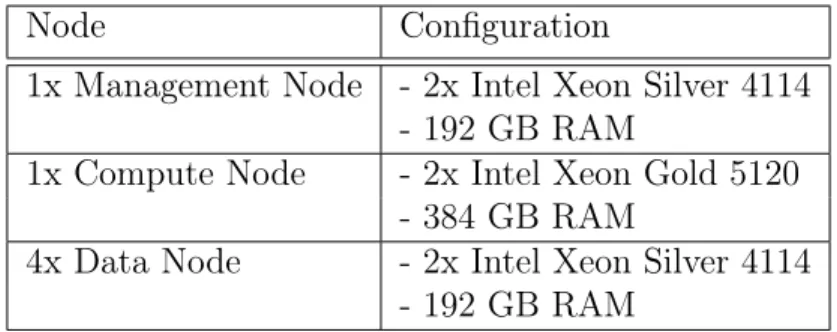
The Hadoop cluster consists of a management node, a compute node and four data nodes. Table 4.1 delineates the configuration of these nodes. A 25Gbit and 10Gbit physical net-works are deployed, interconnecting the nodes. The former network is primarily used for data and applications, while the latter one is for administration.

Table 4.1: Hardware Configuration of the Hadoop Cluster

Node Configuration

1x Management Node - 2x Intel Xeon Silver 4114 - 192 GB RAM

1x Compute Node - 2x Intel Xeon Gold 5120 - 384 GB RAM

4x Data Node - 2x Intel Xeon Silver 4114 - 192 GB RAM

(34)

4.1.2 Software

The software implementation is primarily based on Java. To ease dependency management, we incorporate Gradle [29]. JGraphT [51] graph library is used to construct the graph and extract graph-based features from network flows. Both Smile [47] and Encog [39] are used in tandem for ML. In order to support rapid prototyping, a custom in-house DataFrame (DataFrame4J) library has been developed. DF4J conforms to the incremental streaming paradigms, data streams with well-defined sources, stages and sinks. Furthermore, the underlying data structures are immutable, and all the basic stream-based transformations are available. More details about DF4J are provided in Appendix A.

4.2 Dataset

The evaluation of BotChase is based on the CTU-13 [33] dataset. CTU-13 comprises of 13 different subset datasets (DS) that include captures from 7 distinct malware, performing port scanning, DDoS, click fraud, spamming, etc. Every subset carries a unique network topology with a certain number of bots that leverage different protocols. Table 4.2 summa-rizes the dataset duration, number of flows and bots, and the type of bot in every subset. CTU-13 labels indicate whether a flow is from/to botnet, background or benign. Known infected hosts are labeled as bots, while the remaining hosts are tagged as benign. We leverage 12 datasets as base training data, while a single dataset, #9, is left out for testing purposes. This test dataset contains NetFlow data collected from a Neris botnet, 10 unique hosts labeled as bots, performing multiple actions including spamming, click fraud, and port scanning. We use this dataset configuration for training and testing, unless stated otherwise.

4.3 Performance

4.3.1 Graph Transform, Feature Extraction & Normalization

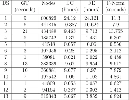
For every subset in the CTU-13 dataset, BotChase first ingests all the network flows, creates the graph, extracts base features and then normalizes them. For each dataset, Table 4.3 highlights the graph creation time i.e., graph transform (GT), number of graph nodes (|V|), total runtime to extract only base BC feature and all base features (FE), and total runtime to normalize features (F-Norm).

(35)

Table 4.2: CTU-13 Dataset

DS Duration # Flows Bot # Bots

1 6.15 2824637 Neris 1 2 4.21 1808123 Neris 1 3 66.85 4710639 Rbot 1 4 4.21 1121077 Rbot 1 5 11.63 129833 Virut 1 6 2.18 558920 Menti 1 7 0.38 114078 Sogou 1 8 19.5 2954231 Murlo 1 9 5.18 2753885 Neris 10 10 4.75 1309792 Rbot 10 11 0.26 107252 Rbot 3 12 1.21 325472 NSIS.ay 3 13 16.36 1925150 Virut 1

Table 4.3: Graph Transform, Base Feature Extraction and Normalization Computation

DS GT Nodes BC FE F-Norm

(seconds) (hours) (hours) (seconds)

1 9 606829 24.12 24.121 11.3 2 6 441845 10.387 10.624 7.9 3 21 434489 9.463 9.713 13.755 4 5 185742 1.37 1.431 6.307 5 1 41548 0.057 0.06 0.556 6 3 107056 0.28 0.295 2.112 7 1 38081 0.021 0.022 0.488 8 13 383339 9.67 9.954 9.617 9 10 366881 8.677 8.97 7.879 10 7 197542 1.06 1.108 4.861 11 1 41809 0.055 0.057 0.627 12 2 94164 0.287 0.302 1.412 13 9 315343 3.667 3.852 6.824

(36)

It is evident that there is a non-linear relationship between BC and the number of nodes in the graph. Furthermore, the inconsistent variation between GT and the number of nodes is due to the differing time windows across datasets. Also, dataset #3 has a much higher number of flows than #2, which increases the runtime of graph creation. This is primarily due to the repeated modification of exclusive flow tuples in set A. The system

then normalizes the base features, and Table 4.3 depicts its total runtime with D = 1.

Evidently, normalizing features does not significantly increase the total runtime of the system. The largest runtime reported for the most complex dataset is 13.755 seconds.

4.3.2 Stand-alone SL

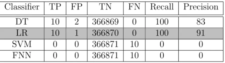
We start by highlighting the limitations of a stand-alone supervised learning approach. This consists of evaluating supervised ML classifiers, including DT, LR, SVM and FNN for bot detection. Each classifier employs graph-based normalized features and is trained on the entire training dataset. In our experiments, DT uses the Gini instance split rule algorithm, LR is used without regularization, and SVM uses the Gaussian kernel with a soft margin penalty of 1. Moreover, NN is configured to use cross entropy as an error function and 10 hidden layers of 1000 units each. Table 4.4 highlights the results, where LR and DT show meaningful classification. Both LR and DT classifiers result in a 100% recall, with 91% and 83% precision, respectively. With LR’s superiority in precision, it seems to be the classifier of choice. The other classifiers were able to accurately classify all the benign hosts, but failed to identify any bots.

Table 4.4: Stand-alone Supervised Learning with F-Norm Classifier TP FP TN FN Recall Precision

DT 10 2 366869 0 100 83

LR 10 1 366870 0 100 91

SVM 0 0 366871 10 0 0

FNN 0 0 366871 10 0 0

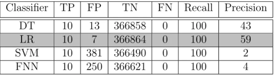
To be fair to SVM and FNN, the input must be balanced. The bots to benign hosts ratio is quite minimal. This heavily affects the bias in the aforementioned classifiers to the benign hosts. To provide balance, we follow a mixed sampling approach. The benign hosts become subject to downsampling to a defined set size (1k, 2k, 5k, 10k). We then perform oversampling with replication for the bots. This provides a balance in between the labels. Given this technique, Table 4.5 depicts the corresponding results.

(37)

Table 4.5: Stand-alone SL with F-Norm and Balanced Input Classifier TP FP TN FN Recall Precision

DT 10 13 366858 0 100 43

LR 10 7 366864 0 100 59

SVM 10 381 366490 0 100 2

FNN 10 250 366621 0 100 4

We find that all the classifiers are viable now. In particular, SVM and FNN are now able to classify bots, albeit with quite a few FPs. DT and LR remain the most promising models after the balancing changes, giving them an edge against the other classifiers.

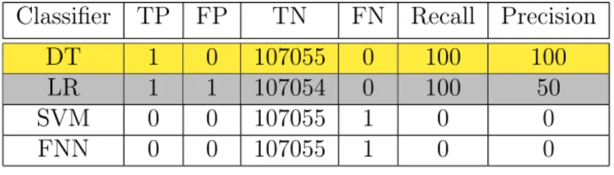
We then evaluate the training time and robustness of the stand-alone classifiers, as depicted in Tables 4.6 and 4.7. DT requires the least training time of 4.9 seconds, which is in high contrast to the 58.2 seconds for LR. That is, DT requires only 8.4% of LR’s training time for the entire training dataset. It is also essential for a bot detection system to detect bots that the classifier has never seen beforei.e., unknown or zero-day attacks. Therefore, to evaluate robustness to zero-day attacks, we change the selection of the training and testing datasets. We choose dataset #6 for testing, which has a unique bot that is not present in any other dataset. The remaining datasets are aggregated to form the training set, with 34 bots and a total of ≈3.1M hosts. Evidently, DT outperforms LR, which misclassifies a benign host, with a low precision of 50%.

Table 4.6: Training Time of Stand-alone Supervised ML Classifiers Classifier Training Time (s)

DT 4.9

LR 58.2

SVM 6832.3

FNN 93

Based on the above evaluations, LR outperforms DT in precision, while DT shows superior training time and robustness to unknown attacks. However, precision, training time and robustness are all crucial for our bot detection system. Can we achieve the best of all three? To investigate this, we set out to evaluate a two-phased system that employs an initial clustering phase (UL), followed by a classification phase (SL). We delineate its evaluation in the following subsections.

(38)

Table 4.7: Stand-alone Supervised Learning against Previously Unknown Bot Classifier TP FP TN FN Recall Precision

DT 1 0 107055 0 100 100

LR 1 1 107054 0 100 50

SVM 0 0 107055 1 0 0

FNN 0 0 107055 1 0 0

4.3.3 Phase 1 (UL)

For Phase 1 in BotChase, we evaluate three UL techniques, namely k-Means, DBScan

and SOM. However, DBScan results are inconclusive, where bots are co-located with be-nign hosts. DBScan is evaluated with varying minimum number of neighborhood points (minPts) and distance (). Multiple values are tested in the range of [10-5, 10-4, ..., 105]. Also, we infer values that correspond to the boundary of the bots themselves. We vary

minPts in [1, 2, ..., 25] depending on the number of bots in the aggregated training dataset. However, maximal separation of bots from benign hosts could not be achieved with the tested parameters. In essence, DBScan does not produce a single, prevalent benign clus-ter. On the other hand, bothk-Means and SOM show appreciable results, where SOM is

trained with a learning rate of 0.7.

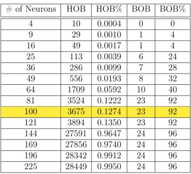
Tables 4.8 and 4.9 highlight the evaluation metrics, including number of clusters or neurons, number of hosts outside the benign cluster (HOB), percentage of hosts outside the benign cluster relative to the total number of hosts (HOB%), number of bots outside the benign cluster (BOB), and percentage of bots relative to the total number of bots (BOB%). Recall, the dataset #9 is removed for testing, which includes 10 hosts labeled as bots and ≈366K hosts. Also, ≈3.2M hosts from the remaining datasets are used to train the classifiers. In comparison to the number of clusters for k-Means, SOM is able

to alienate its first bot outside the benign cluster with a lower number of neurons (9 vs. 16). With 81 neurons, SOM has a recall rate of 92% compared to the 42% of k-Means.

However,k-Means catches up with 121 clusters. Nevertheless, SOM outperformsk-Means

by maximizing the number of bots isolated with a smaller number of neurons.

With a cluster size of 100,k-Means alienates 21 bots, while having an outside host sum

of 3028 for the remaining non-benign clusters. In contrast, SOM removes 23 bots from the benign cluster with an outside host sum of 3675. The very next k-Means cluster size

i.e., 121, boosts HOB from 3028 to 26935, while SOM remains at a close 3894. However,

k-Means isolates three extra bots, yielding 24 BOB for 26935 HOB. That is, three extra

(39)

Table 4.8: k-Means Clustering with F-Norm

# of Clusters HOB HOB% BOB BOB%

4 5 0.0002 0 0 9 12 0.0004 0 0 16 36 0.0012 1 4 25 94 0.0033 6 24 36 170 0.0059 6 24 49 473 0.0164 8 32 64 1071 0.0371 10 40 81 1133 0.0392 10 40 100 3028 0.1049 21 87.5 121 26935 0.9327 24 96 144 27100 0.9384 24 96 169 27302 0.9454 24 96 196 27359 0.9474 24 96 225 28752 0.9956 24 96

Table 4.9: SOM Clustering with F-Norm # of Neurons HOB HOB% BOB BOB%

4 10 0.0004 0 0 9 29 0.0010 1 4 16 49 0.0017 1 4 25 113 0.0039 6 24 36 286 0.0099 7 28 49 556 0.0193 8 32 64 1709 0.0592 10 40 81 3524 0.1222 23 92 100 3675 0.1274 23 92 121 3894 0.1350 23 92 144 27591 0.9647 24 96 169 27856 0.9740 24 96 196 28342 0.9912 24 96 225 28449 0.9950 24 96

(40)

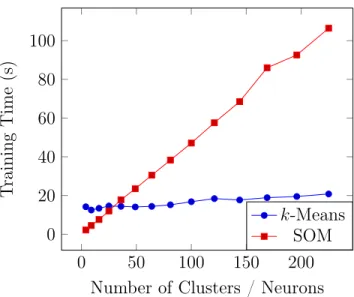
0 50 100 150 200 0 20 40 60 80 100

Number of Clusters / Neurons

Training

Time

(s)

k-Means

SOM

Figure 4.1: Comparison of SOM andk-Means with respect to training time

jointly minimize HOB while maximizing BOB. Therefore, SOM with 100 neurons becomes the natural choice.

With respect to runtime, k-Means mostly outperforms SOM, as depicted in Fig. 4.1.

With 100 clusters, k-Means took 16.8 seconds to train, in comparison to 47.1 seconds

of SOM. We speculate that SOM’s ever increasing training time is attributed to how it updates the surrounding neurons. As the number of neurons increases, the density of their neighborhood also increases. Eventually, more neurons will tend to be within the threshold radius. Nevertheless, with recall being our top priority, we leverage SOM as UL classifier in Phase 1.

4.3.4 Phase 2 (SL)

The training set for Phase 2 is determined by the number of hosts outside the benign cluster in Phase 1. These are the relevant hosts for this phase, as hosts that are assigned in the benign cluster never make it to Phase 2. With a 10×10 (i.e., 100 neurons) SOM and normalized features in Phase 1, the size of the dataset is significantly reduced. Therefore, we have 3675 HOB, including 23 bots, for further classification in Phase 2.

The DT classifier shows the best performance with the small dataset, as depicted in Table 4.10. It successfully detects all bots in the test dataset, with only a single FP out of the 366871 benign hosts. In contrast, all other classifiers are lackluster and unable to recall

(41)

Table 4.10: Supervised Learning with F-Norm Classifier TP FP TN FN Recall Precision

DT 10 1 366870 0 100 90.9

LR 0 0 366871 10 0 0

SVM 0 0 366871 10 0 0

FNN 0 0 366871 10 0 0

even a single bot from the dataset. We believe this is because all classifiers, except DT, rely on gradient-descent for error-correction. This implies that every single node in the dataset will affect the end-hypothesis function. Thus, with a dataset that is unbalanced, the hypothesis will be biased towards the benign hosts, which is the case for LR, SVM and FNN. Table 4.11 shows the results with a balanced training dataset in this current scenario. SVM and FNN remain unfazed, not being able to classify a single bot. However, DT shows a significant depreciation of its classification performance. Since this is the pruned dataset, the number of unique data points present is minimal and the imbalance isn’t as significant as that observed in the previous standalone SL section. As DT incurs a significantly less training time than LR, we proceed with the vanilla pruned dataset in the following analyses.

Table 4.11: Supervised Learning with F-Norm on the Balanced Dataset Classifier TP FP TN FN Recall Precision

DT 1 0 366871 9 10 100

LR 10 9 366862 0 100 53

SVM 0 0 366871 10 0 0

FNN 0 0 366871 10 0 0

Table 4.13 highlights the training time for the supervised classifiers. For Phase 1, a 10×10 SOM incurs a training time of 47.1 seconds, while DT has the lowest training time of 88 milliseconds in Phase 2. Thus, the aggregate training time for both phases is ≈47.2 seconds. This is an 11 seconds improvement over the 58.2 seconds observed for a stand-alone LR classifier [11].

Using dataset #6 for testing, the robustness test harbors more hosts for training in Phase 2. Most importantly, there are more BOB, yielding a higher ratio of bots to hosts outside the benign cluster, as depicted in Table 4.12. The robustness results are portrayed in Table 4.7. Though LR is able to recall the malicious bot while incurring only a single FP,

(42)

Table 4.12: SOM with Newly Aggregated Dataset # of Neurons HOB HOB% BOB BOB%

100 3769 0.0011 32 94.12

Table 4.13: Training Time of Supervised Classifiers on the Pruned Dataset Classifier Training Time (ms)

DT 88

LR 2454

SVM 864

NN 3278

DT exhibits perfect results on this specific test dataset. It is able to detect the previously unknown bot, as well as correctly classify all the benign hosts. Therefore, with SOM selected for Phase 1 and DT for Phase 2, the system ensures minimal training time and robustness to unknown attacks, with high recall and precision.

4.3.5 Feature Normalization

Recall that aggregating datasets from different networks can negatively impact the base features, thus compromising system performance. Essentially, the topological structure of different networks affect the extracted graphical features, greatly skewing bot pattern and behavior. Thus, the intuition behind feature normalization is to make hosts, including bots, from different datasets look alike.

Table 4.14 showcases the crucial depreciation of the SOM results without normalizing graph-based features. For example, with 81 neurons, SOM with and without F-Norm scores 92% and 60% on BOB, respectively. On average, the results without F-Norm have a higher HOB. This intrinsic observation signifies the lack of similarity between hosts of the same category. For example, benign hosts from different networks are not co-located due to the stark differences in their features. Conversely, with F-Norm, similarly labeled hosts are more frequently co-located, yielding better BOB and HOB. Hence, normalized graph-based features significantly improve the spatial stability of ML in BotChase.

For 100 neurons, SOM with Norm results in 23 BOB and 3675 HOB. Without F-Norm, it results in 22 BOB and 8465 HOB, as shown in Figures 4.2 and 4.3. Thus, for the

(43)

Table 4.14: SOM Clustering without F-Norm # of Neurons HOB HOB% BOB BOB%

4 8 0.0003 0 0 9 39 0.0014 0 0 16 689 0.0239 0 0 25 935 0.324 0 0 36 2280 0.0790 9 36 49 3792 0.1315 11 44 64 4207 0.1459 14 56 81 6721 0.2333 15 60 100 8465 0.2940 22 88 121 12923 0.4495 24 96 144 20780 0.7248 24 96 169 22607 0.7890 24 96 196 23714 0.8280 24 96 225 42125 1.4803 24 96

same number of neurons, feature normalization was able to maximize BOB, while mini-mizing HOB. Therefore, we choose 100 neurons with F-Norm as our primary configuration for SOM.

4.3.6 Feature Engineering

It is important to gauge the significance and impact of the chosen graph-based features on bot detection. Albeit different feature combinations may impact the results, are all features necessary? Table 4.15 shows the Pearson’s feature correlation matrix for the normalized graph-based features. At a glance, we can determine that the first five features are highly correlated, with a correlation close to or greater than 0.9. Therefore, feature combinations that exclude some of these features may not exacerbate classification accuracy. On the other hand, the last two features are highly uncorrelated, with LCC being the least correlated. Hence, we start with removing IDW and ODW, which decreases the benign cluster size but results higher on BOB, as shown in Table 4.16. However, Table 4.17 shows the lackluster performance of the SL classifiers when we eliminate IDW and ODW features. Precision drops to 52.6% for DT from 90.9% (cf., Table 4.10). Also, LR now misclassifies two benign hosts as bots.

(44)

0 50 100 150 200 0 1 2 3 4 ·104 Number of Neurons HOB With F-Norm Without F-Norm

Figure 4.2: Number of hosts outside the benign cluster (HOB) assigned by SOM with and without feature normalization

0 50 100 150 200 0 5 10 15 20 25 Number of Neurons BOB With F-Norm Without F-Norm

Figure 4.3: Number of bots outside the benign cluster (BOB) assigned by SOM with and without feature normalization

(45)

Table 4.15: Pearson’s Feature Correlation Matrix with F-Norm ID IDW OD ODW BC LCC AC ID 1 0.99 0.92 0.95 0.96 0.03 0.32 IDW 0.99 1 0.91 0.96 0.97 0.03 0.33 OD 0.92 0.91 1 0.89 0.90 0.08 0.37 ODW 0.95 0.96 0.89 1 0.97 0.04 0.43 BC 0.96 0.97 0.90 0.97 1 0.01 0.46 LCC 0.03 0.03 0.08 0.04 0.01 1 0.01 AC 0.32 0.33 0.37 0.43 0.46 0.01 1

Table 4.16: SOM Clustering without IDW and ODW # of Neurons HOB HOB% BOB BOB%

100 27404 0.958 24 96

Table 4.17: Supervised Learning without IDW and ODW Classifier TP FP TN FN Recall Precision

DT 10 9 366862 0 100 52.6

LR 0 2 366869 10 0 0

SVM 0 0 366871 10 0 0

(46)

A weakness of the chosen features is the runtime of BC. For the first dataset, it took over 24 hours to compute BC. This will render any effort to expedite the learning process in vain. However, removing BC from the feature set adversely affects the performance of DT, but not for SOM, as depicted in Tables 4.18 and 4.19. SOM without BC performs identical to the use of the entire feature set. On the other hand, DT’s precision is affected by the removal of BC, but it is better than that of the removal of IDW and ODW from the feature set. While the precision deteriorated,only 6 and 9 benign hosts were misclassified out of the ≈367K hosts with the removal of BC and IDW/ODW, respectively. This reinforces the correlation matrix i.e., having these features the most correlated. Since recall and precision are sought after metrics in BotChase, it is important to include these features for training and testing classifiers.

Table 4.18: SOM Clustering without BC # of Neurons HOB HOB% BOB BOB%

100 3622 0.125 23 96

Table 4.19: Supervised Learning without BC Classifier TP FP TN FN Recall Precision

DT 10 6 366865 0 100 62.5

LR 0 0 366869 10 0 0

SVM 0 0 366871 10 0 0

FNN 0 0 366871 10 0 0

4.4 Comparative Analysis

Given the modularity of BotChase, in-place substitution of modules is possible. For exam-ple, rather than having graph-based features, the system can leverage flow-based features, while maintaining the two-phased bot detection. Therefore, we first compare the perfor-mance of our graph-based features with flow-based and hybrid features from BotMiner and BClus in BotChase. Furthermore, we compare BotChase with the end-to-end system proposed for BClus. Finally, we provide a rough comparison against BotGM. For a fair comparison, we reselected the training and testing datasets. This conforms to the selection in [33], where the test dataset contains multiple bot types and different network topologies. The dataset selection of these comparisons is depicted in Table 4.20.

(47)

Table 4.20: Comparative Training and Testing Datasets Purpose Dataset

Training 3,4,5,7,10,11,12,13 Testing 1,2,6,8,9

BotMiner aggregates flows based on their source IP, protocol, destination IP and its corresponding port. These aggregated flows, called C-Flows, are processed in a time epoch that lasts up to a full day of flow capture. After flows are aggregated, 52 features are extracted by first mapping every C-Flow into a discrete sample distribution of four random variables: (i) total number of packets sent and received in a flow, (ii) average number of bytes per packet, (iii) total number of flows per hour, and (iv) average number of bytes per second. These random variables are then binned into 13 slots according to pre-defined percentiles. Through this technique, every variable is converted into a vector of 13 elements, totaling 52 features per C-Flow.

BClus undertakes a similar clustering approach by grouping flows into instances. These instances are identified by unique source IPs in a certain time window. Each instance is represented using 7 features: (i) source IP address, (ii) number of distinct source ports, (iii) number of distinct destination ports, (iv) number of distinct destination IPs, (v) total number of flows, (vi) total number of bytes, and (vii) total number of packets. These instances are then clustered using Expectation Maximization (EM). More features are then extracted from the clusters themselves to aid JRip, a propositional rule learner, in their labeling. These features include: (i) total number of instances, (ii) total number of flows, (iii) number of distinct source IP addresses, and (iv) the average and standard deviation amount of distinct source ports, distinct destination IPs, distinct destination ports, number of flows, number of bytes, and number of packets. Hence, every cluster exhibits 15 features, which are then used by JRip. After training, JRip is capable of classifying each cluster as malicious or benign. Ground truth label of clusters is determined through a bot flow threshold that is varied to find the best JRip model.

BotGM uses graph-based outlier detection to detect suspicious flow patterns. It starts off with extracting events, i.e., converting flows into a key-value entry. The key represents the source and destination IPs while the value represents the source and destination ports. Then, a sequence is extracted that tracks the source and destination port variations of two unique IPs. A directed graph is then extracted from these variations, with vertices representing a port 2-tuple. The aggregate graphs are then mined for outlier detection. They use the graph edit distance to gauge how different a graph is from another. The

(48)

inter-quartile method is then used to detect outliers.

4.4.1 BotMiner Flow-Based vs. Graph-Based Features

We start with the aforementioned flow-based features from BotMiner in BotChase. Ta-ble 4.21 showcases the outcome of classifying flows using BotMiner features, where only LR is able to detect a few malicious flows, misclassifying the majority of benign and malicious flows. To compare, we convert our host classification into flow classification in Table 4.22. With a recall (RCL) of 0.02% and a precision (PRC) of 16.28%, BotMiner features perform poorly against the graph-based features. The latter scores 81.57% and 99.51% on recall and precision, respectively. However, in comparison to host classification (cf., Table 4.26), the precision is significantly higher as the flows originating from the identified FP hosts were relatively minimal. Likewise, the different number of flows per host may result in a lower or higher recall rate. While LR and DT highlight similar host classification results, DT is the more favorable flow classifier as it does not misclassify prominent benign hosts.

Table 4.21: Supervised Learning with BotMiner Features without F-Norm

Classifier TP FP TN FN RCL PRC

DT 0 1 2550094 34966 0 0

LR 7 36 2550059 34959 0.02 16.28

SVM 0 0 2550095 34966 0 0

FNN 0 0 2550095 34966 0 0

Table 4.22: Flow-Based Supervised Learning

Classifier TP FP TN FN RCL PRC

DT 211452 1037 20145929 47776 81.57 99.51 LR 67006 59657 20087309 192222 25.85 52.9

SVM 0 0 20146966 259228 0 0

FNN 0 0 20146966 259228 0 0

4.4.2 BClus Flow-Based vs. Graph-Based Features

Implementing BClus features in BotChase was an incremental process. Alongside choosing the optimal number of EM clusters, F-Norm had a major impact on the results. Unlike

(49)

BotMiner, BClus strictly classifies instances pertaining to unique source IPs. Using a large time window that fits the entire test dataset, an instance becomes a full representation of host behavior. As depicted in Table 4.23, our preliminary implementation of BClus without F-Norm had a zero recall rate across all the trained supervised classifiers. Therefore, to improve BClus we modified F-Norm to process all the hosts.

Recall that BClus extracts features for source IPs only, thus features of destination IPs are missing from our data pipeline. The data pipeline only consists of hosts that have had their features extracted based on previous aggregations. Hence, a direct application of F-Norm, as implemented in BotChase, results in missing data elements for hosts that are present in the graph but not in the data pipeline. Therefore, we first naïvely modify F-Norm to handle non-existent data points with a zero vector. This improves the results of LR, which now captures a single bot out of 14, while the remaining classifiers still perform poorly, as depicted in Table 4.24. This comes with no surprise, as a zero vector still affects the relative values of the host features.

Finally, we transform BClus to account for both source and destination IPs as instances. This solves the issue with F-Norm, since all unique IPs in the network are mapped into a corresponding data point and host node in the graph. Using this two-way analysis, Table 4.25 shows an appreciable improvement over the former iterations. DT manages a jump from 0% to 64.29% in recall and 81.82% in precision. However, even after the improvements to BClus features, it significantly underperforms our graph-based features. Table 4.26 showcases the performance of the graph-based features on the new dataset selection. It exhibits convincing results for both DT and LR, with high rates of 85.71% and 80% on recall and precision, respectively.

Interestingly, DT and LR have similar performance on host classification yet different on flow classification. Although both classifiers agree metrics-wise, the underlying sets of hosts tagged as bot or benign are different. Hence, it is possible to combine the classifiers into a single decision making entity. A simple rule to boost our classification results could be to flag a host as a bot if at least one classifier concurs. While this can potentially increase the recall rate, precision is expected to decline as FPs are aggregated across classifiers.

4.4.3 BClus Hybrid vs Graph-Based Features

So far, we have experimented with both BClus’ flow-based features and BotChase’s graph-based ones. How would they fair if paired in the same ML model? With 6 flow-graph-based and 7 graph-based features, every unique host in the network depicts 13 features to be processed by the system. In this experiment, we resort to BotChase as our base architecture, only

BotChase: Graph-Based Bot Detection Using Machine Learning