Support Vector Machine Histogram: New Analysis
and Architecture Design Method of Deep
Convolutional Neural Network
著者(英)
Satoshi Suzuki, Hayaru Shouno
journal or
publication title
Neural Processing Letters
volume
47
number
3
page range
767-782
year
2017-07-03
URL
http://id.nii.ac.jp/1438/00008915/
doi: 10.1007/s11063-017-9652-0(will be inserted by the editor)
Support Vector Machine Histogram:
New Analysis and Architecture Design Method of
Deep Convolutional Neural Network
Satoshi Suzuki · Hayaru Shouno
Received: date/Accepted: date
Abstract Deep Convolutional Neural Network (DCNN) is a kind of hierarchical neural
network models and attracts attention in recent years since it has shown high classification performance. DCNN can acquire the feature representation which is a parameter indicating the feature of the input by learning. However, its internal analysis and the design of the net-work architecture have many unclear points and it cannot be said that it has been sufficiently elucidated. We propose the novel DCNN analysis method “Support Vector Machine (SVM) Histogram” as a prescription to deal with these problems. This is a method that examines the spatial distribution of DCNN extracted feature representation by using the decision bound-ary of linear SVM. We show that we can interpret DCNN hierarchical processing using this method. In addition, by using the result of SVM Histogram, DCNN architecture de-sign becomes possible. In this study, we dede-signed the architecture of the application to large scale natural image dataset. In the result, we succeeded in showing higher accuracy than the original DCNN.
Keywords Deep Convolutional Neural Network·Support Vector Machine·Architecture
Design·CIFAR-10·ImageNet
1 Introduction
Deep Convolutional Neural Network (DCNN) is one of the multi-layer neural networks, which can automatically obtain feature representation from input data [3]. The origin of DCNN is known as “Neocognitron”, which is proposed by Fukushima [5, 12]. Neocog-nitron is a visual model of “Simple Cell” and “Complex Cell” discovered by Hubel and Wiesel, in the cat’s primary visual cortex and monkey’s V1 field and it realized with the
University of Electro-Communications Chofugaoka 1-5-1, Chofu, Japan University of Electro-Communications Chofugaoka 1-5-1, Chofu, Japan Tel.:+8142-443-5787 Fax:+8142-443-5787 E-mail: [email protected]
framework of a hierarchical neural network. They are implemented by Convolution oper-ation and Pooling operoper-ation, respectively. In recent years, the DCNN model represented by AlexNet proposed by Krizhevskyet al. which attracts attention because it shows clas-sification accuracy exceeding other methods without DCNN in the contest such as image classification and speech recognition [11, 18]. The DCNN is now going to become ade facto standardclassification tool in the image classification field, and the related research has been increased [3].
DCNN has been shown to be an effective model for image classification, speech recog-nition, furthermore computer games [16], etc. However, it is known that the following prob-lems exist [18].
1) Since the processing and behavior inside DCNN are very complicated, it is difficult to analyze how to obtain high classification accuracy.
2) Since there are few design guidelines with respect to the architecture of DCNNs, it is necessary to do trial-and-error many times.
In this work, in order to deal with these problems, we consider applying the analysis method of internal behavior of DCNN using the linear Support Vector Machine (SVM) proposed in the previous work, and we call this method “SVM Histogram” [15]. SVM Histogram is a technique to make the decision boundary of linear SVM using the feature extracted from the inside of the DCNN and to investigate the spatial distribution of the feature representation by projecting it to the decision boundary.
In the previous work, we analyzed by investigating the progress of pattern separation between layers by using this SVM Histogram, and we revealed that DCNN is promoting class separation by making narrow the histogram shape for each layer [15]. As the result, we concluded the narrower representation of each class plays an important role for the class discriminability.
In this work, we analyze the internal representation of DCNN using this SVM Histogram and investigate how obtains the feature representation acquired not only changes from layer to layer but also in the learning process. In addition, we apply our method to architecture design of DCNN and try to utilize it as the guideline for architecture design.
1.1 Related Work
In this subsection, we introduce the related research on DCNN analysis method and archi-tecture design.
1.1.1 Interpretation of representation in DCNN
In order to make it possible to interpret the feature representation of DCNN, many types of research have been done on visualization of feature representation in previous works. Visualizing the feature representation of the DCNN intermediate layer is extremely useful because it can intuitively evaluate what kind of feature representation hierarchically acquired by DCNN. However, the technique of simply visualizing the convolution filter can only be applied to the first layer closest to the input pixel space. As a visualization method of high layer filters, Zeileret al.proposed Deconvolutional network (DeconvNet) which is a method of simulating feedback of the DCNN forward propagation process, and revealed that feature representation of different abstraction levels is extracted for each layer [18]. This method is
intuitive in that it shows image features that react of intermediate layers, but it is unclear as to how these features contribute to classification.
On the other hand, Linet al.proposed a classification method that classifies by taking the average value from the entire feature map, which is the processing result of the Con-volution operation [13]. By visualizing the feature map before taking the average value of this method, it was clarified which part of the input image contributes to classification. In addition, Simonyanet al.proposed a method to optimize the input image so as to maximize the classification probability of each category and visualize which features of each category are responsive selectively in DCNN recognition layer [17]. In contrast to the above method, these methods can investigate which part of the input image contributes to the classification, but there is a problem that changes in the feature expression in the layerwise processing of DCNN cannot be visualized.
In this work, we propose a method to visualize the feature representation as a projec-tion of the distance to the decision boundary of the linear SVM, rather than showing the feature representation like above methods as an image. By using this method, we can obtain separation information of feature representation of each layer.
1.1.2 Architecture Design
The architecture design of DCNN is a very important factor influencing the classification accuracy of it. However, in the architecture design of DCNN, there are few design guide-lines except the classification accuracy when learning converges. Therefore, the architecture design of DCNN has found a better architecture by a large number of trial-and-error at present [18].
In order to deal with this problem, Zeiler et al. showed that the classification accu-racy improves by modifying the architecture so as to reduce the filter which does not con-tribute to feature extraction among the AlexNet filters using the visualization result of De-convNet [18]. In the case of improving the architecture using DeDe-convNet, it is possible to modify the local architecture such as the size and stride of the convolution filter, but it is difficult to alter the global architecture such as a combination of Convolution and Pooling layers. In addition, it is relatively difficult to find a way to improve DCNN from the ob-tained results, and it is predicted that it will be difficult to utilize unless you are familiar with DCNN.
On the other hand, by using unsupervised learning method like Fukushima’s Add-if-Silent (AiS) rule, it becomes possible to automatically obtain the number of filters, that can sufficiently express input data. The AiS rule is a method of incrementing the corresponding filter sequentially until there is no feature extraction filter that responds to input data [6]. Un-supervised learning method such as AiS rule is capable of designing architectures according to the nature of input data but similar to the method of Zeileret al., there are problems such as the number and the combination of layers to be determined in advance. Also, as com-pared with supervised learning, label information is missing, so classification accuracy is often inferior.
2 Method and Formulation
2.1 Deep Convolutional Neural Network
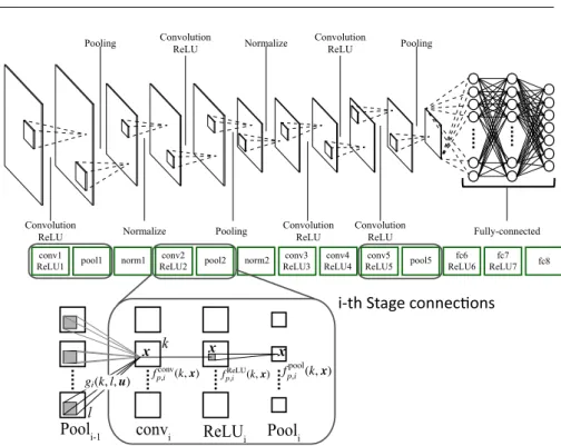
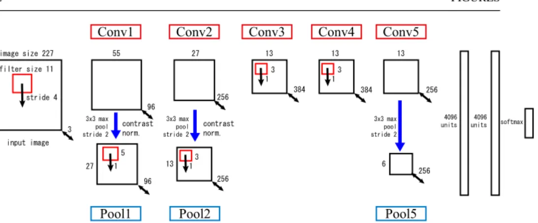
In this work, we use the CaffeNet as the baseline DCNN [4]. This CaffeNet has an almost same architecture to the AlexNet [11]. And Fig.1 shows the CaffeNet architecture. Here, we explain and formulate the components of DCNN by taking CaffeNet as an example.
The DCNN has an alternate structure of pattern transformation called “stage” [5, 14], which basically consists of “Convolution”, “Rectified Linear (ReLU)”, and “Pooling” lay-ers. Considering theith stage for thepth input pattern, we formulate each layer response as followings. The “convolution” layer extracts feature maps as
fpconv,i (k,x)=X
l,u
gi(k,l,u) fppool,i−1(l,x−u), (1)
wherek means the index of feature map, andxmeans the location of the map. The con-volution kernelgi(k,l,u) means the feature including in thelth feature map of the pooling
(with normalization) layer in the previous stage fppool,i−1(l,x) . In each feature map fconv
p,i (k,x),
extracted features are modulated with the rectified linear unit (ReLU):
fpReLU,i (k,x)=max[0,fpconv,i (k,x)+bi,k], (2)
wherebi,k means bias parameter ofkth index. Then, in each modulated feature map,
spa-tially neighbor responses are gathered for calculation of representative value, which is called spatial pooling:
fppool,i (k,x)= max
ξ∈N(x)[f ReLU
p,i (k,u)], (3)
where N(x) means the spatial neighbor area around the locationx on the map. We call the pooling method as described above as “max-pooling”. In addition to this, there is a method called “average-pooling” whose representative value is the average value of the space neighborhood regionN(x). Then, these response maps are normalized in the same manner with Krizhevskyet al.at optional [11].
In the Fig.1, “fc6”, which abbreviate 6 th stage fully-connected layer, is feature extrac-tion layer. Following layers, which are “fc7”, “fc8” layers, have the multi-layer perceptron (MLP) structure, which plays a role as the classier. In this work, we fixed the training method for the DCNN as the error back-propagation (BP) method, which is used as the standard training method in these decades [12].
Also, there are parameters called Stride and Filter size for Convolution and Pooling processing of DCNN. Stride parameter is the distance between the Convolution (or Pooling) filter centers of neighboring processes in a input feature map [11], Filter size is a parameter that determines the size of filter. For example, the filter on the Conv1 layer of CaffeNet has Stride:4 and Filter size:11×11.
2.2 Layer Response Representation with SVM Histogram
This section explains the SVM histogram for layer representation in the DCNN [15]. In the previous work, we introduced a linear SVM for each layer in order to observe how representations in the DCNN develops throughout layer transformations. Let us consider the linear SVM which finds a decision boundary. The decision boundary is described asy(x)=
wtφ(x)+b= 0, whereφ(x) denotes the layer representation for the input patternx. Here
we introducetas the teacher signal, which is described astn ∈ {1,−1}in the case of
two-class two-classification problem wherenmeans the index for the test class pattern. In the feature space, the decision boundary of the linear SVM is obtained by maximizing the margin, 1/||w|| minn[tn(wTφ(xn)+b)] [1]. Please note that we use the one-vs-one classification
method for linear SVM training of SVM Histogram.
In our previous work, we introduced a distance from the decision boundary for each layer representation φ(x) as a measure of discriminability, which is described as y(x) =
wTφ(x)+bwherewandbare optimized by the linear SVM. Then, we can obtain a test class projection{y(xn)}. We analyze the projection{y(xn)}as a histogram in the previous
work[15]. Hereafter, we call it as “SVM Histogram” for layer representation. Using the SVM Histogram for each layer, we can visualize the distribution of each class data for an intermediate layer of the DCNN. Here, Fig.2 shows the overview of the SVM histogram.
[Fig. 2 about here.]
According to the previous work, the SVM histogram becomes narrower through the hierar-chical development of representation in the DCNN layers. As the result, we concluded the narrower representation of each class plays an important role for the class discriminabil-ity [15].
3 Feature Analysis with SVM Histogram
First of all, we try to analyze the internal representation of DCNN using SVM Histogram. We use CIFAR-10 dataset [9, 10] as training and evaluation dataset, and investigate how class separation progresses with the number of learning. This CIFAR-10 dataset is often used for DCNN evaluation, and it is one of the benchmarks of DCNN and related technologies [7, 13]. In addition, the data size is about 200 MB, it is very light compared to ImageNet and if you want to do a replicate experiment, there is also an advantage that it is extremely easy to do.
3.1 Training Details
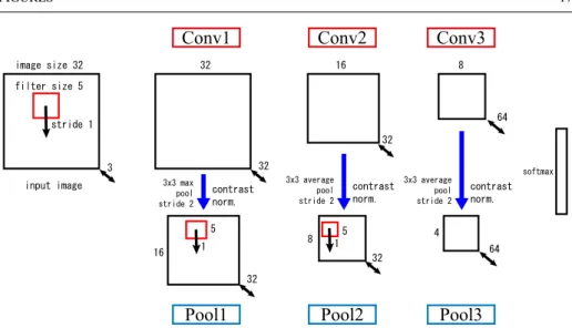
In the following, we describe the details of the learning of DCNN, which is carried out in this section. Fig.3 shows the DCNN architecture in this experiment. This model is trained with the CIFAR-10 training set (10 classes, 60,000 images), and the classification accu-racy is evaluated using the 10,000 images [9, 10]. Each 32×32 [pixel] RGB image was subtracted the per-pixel mean as preprocessing. In the BP training, stochastic gradient de-scent with mini-batch of size 100 is used to update the parameters. In addition, the learn-ing rate starts with 10−2, the momentum parameter is set to 0.9, and we anneal the
learn-ing rate withγ = 0.1 in 60,000 and 65,000 iterations. These implementations and learn-ing methods follow caffe’s default settings [8], and this architecture has the same struc-ture as cuda-convnet proposed by Krizhevsky. Since the almost cuda-convnet’s web page
cannot be browsed now, please refer to caffe’s web page for details of network structure
(http://caffe.berkeleyvision.org/gathered/examples/cifar10.html).
[Fig. 3 about here.]
3.2 Evaluation Data
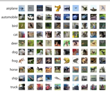
We randomly collected 100 images of each class from the test image of the CIFAR-10 dataset, 50 of which were used for learning linear SVM and the other half for making SVM Histogram. Examples of the image used to create SVM Histogram is shown in Fig.4.
[Fig. 4 about here.]
3.3 Analysis of DCNN Feature Representation
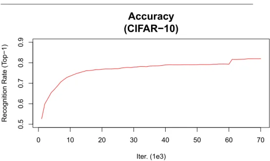
First, the Fig.5 shows the classification accuracy of the model of Fig.3 learned with the CIFAR-10 training dataset. After 70,000 iterations training, this model has obtained about 82.0% classification accuracy, which is consistent with Krizhevsky’s report [10]. In addition, it is expected that convergence of learning is seen even if we look at the transition of accuracy from Fig.5.
[Fig. 5 about here.]
Next, we extracted the feature representation from the Conv layers and the spatial Pool layers having the same structure as Neocognitron using the evaluation data described in Subsection3.2. And we created SVM Histogram using these feature representation. Also, to investigate the differences in the learning process, feature representation was extracted from three types of DCNN, 1,000, 10,000 and 70,000 iterations training. Fig.6 is the SVM Histogram in the classification problem between the “airplane” class and “automobile” class. In Fig.6, each row shows the same iteration and each column shows the same layer. And the red histogram makes from the data of the airplane class, the blue one makes from the data of the automobile class. From Fig.6, in the feature representation extracted from the lower layer, class separation is hardly performed, but we can see that gradual separation is obtained after going through the hierarchy. Furthermore, the features of the 70,000 iterations, which has advanced learning, histograms becomes narrower than those of the 1,000 and 10,000 iterations. In another word, we can guess that within-class variance of DCNN of 70,000 iterations is smaller than other two DCNNs.
[Fig. 6 about here.]
In addition to the above qualitative evaluation, we also evaluate the result quantitatively in following way. For the evaluation, we focus the separability of the histogram clusters. We calculate within-class variances of the histograms, at first. Denoting the distace from the SVM discrimination boudary asrci, whereiandcmean the pattern and class ids respectively, we can derive the witin-class variances2as
mc= 1 Ni X i rci, (4) (sc)2=X i (rci−mc)2, (5) S =X c (sc)2. (6)
For comparison, we also calculate the other separation criterion, that is the ratio between within- and between-class variaces. This criterion is known as linear discriminatnt analsys (LDA). We also calculate the value for the classc1andc2asJc1,c2as
Jc1,c2= (mc1−mc2)2 (sc1)2+(sc2)2 (7) J= X (c1,c2) Jc1,c2, (8)
where the notation (c1,c2) in the summation means the whole combination of class pairs.
The upper part of the fig.7 shows the box plot of the ratio criterionJ, and the lower part shows the one for theS, which means the within-class variance histogram for all combi-nations of SVM histograms. In each graph, the horizontal axis shows the layer index of extracted feature representation, and the vertical one shows the criterion value. From the upper part of the Fig.7, we can see the criterionJ reduces through the transformation, and the differences among the training epochs is not clear. From the lower part of Fig.7, same as in the above qualitative evaluation, as the learning progresses, we can see that the SVM Histogram becomes narrower and the within-class variance decreases more clear. We can also see that especially the within-class variance in the Pool layer decreases remarkably. In other words, it became clear that as the learning converged, the within-class variance of SVM Histogram decreases and class separation was proceeding. Also, paying attention to boxplot of DCNN that has performed 70,000 iterations learning, the within-class variance of the Conv2 layer and the Conv3 layer has hardly changed, and seemingly the class separa-tion has not progressed. However, looking at the Pool2 and 3 layers, it can be seen that the within-class variance of the Pool3 layer is smaller than the Pool2 layer. Actually, from Fig.6, also the histograms become narrower in the Pool3 layer than in the Pool2 layer, so it can be said that better class separation has been achieved. From these facts, DCNN is thought to be able to acquire characteristic expressions with better class separation performance when the within-class variance of SVM Histogram shift while increasing or decreasing rather than staying constant at a low level.
[Fig. 7 about here.]
4 Experiments for Large Scale Natural Image Dataset
In this section, we use CaffeNet [4] which has the almost same architecture as AlexNet to learn ImageNet 2012 which is a large scale natural image dataset.
4.1 Training Details
Here, we describe details of DCNN learning performed in this section like Subsect. 3.1. Fig.8 and Fig.12 show the architectures in this experiment. These models are trained with the ImageNet 2012 training set (1.3million images, spread over 1000 different classes), and the classification accuracies are evaluated using the 50,000 images [2, 11].
Each RGB image was pre-processed by resizing 256×256 [pixel], subtracted the per-pixel mean (across all images) and cropping out the 227×227 [pixel] from the center. In the BP training, stochastic gradient descent with mini-batch of size 256 is used to update the parameters. In addition, the learning rate starts with 10−2, the momentum parameter is set
to 0.9, and we anneal the learning rate withγ=0.1 for stepsize 150,000 and stop training after 450,000 iterations.
[Fig. 8 about here.]
4.2 Evaluation Data
To evaluate the SVM histogram, we extract 50 images from each 10 classes of “Tench”, “Goldfish”, “Brambling”, “Black swan”, “Tusker”, “Echidna”, “Platypus”, “Wallaby”, “Koala”, and “Wombat” from the ImageNet 2012 validation dataset. From the 500 image, we divide them into the 2 datasets. One is used for the linear SVM training, and the other is used for the evaluation of the SVM histograms. Each dataset has 250 images without overlapping. Fig.9 shows several examples used in the experiments.
[Fig. 9 about here.]
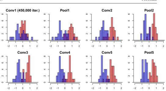
4.3 Evaluation of Class Separation
As described in the Subsect.4.2, we evaluate the SVM histogram with the subset of the ImageNet 2012 dataset. Fig.10 shows the histograms results for the classifier of “Tench” and “Goldfish” classes. Here, we used the CaffeNet with 450,000 iterations training. In each histogram, the horizontal axis shows the location of the data from the decision boundary, where the origin indicates the decision boundary, and the vertical one shows the frequency of the test class examples. The histograms of Conv1 to Pool5 layers feature representation are shown from the upper left to the lower right. From Fig.10, in low layers of CaffeNet, the class separation is not enough, however, we can see that it gradually improves through the hierarchy. Also, in Pool2 and 5 layers, the histogram becomes narrower and it is understood that the class separation is progressed, but in the Pool1 layer, it seems that the within-class variance increases rather than decreases. In addition, we can see that class separation was hardly advanced from the results of SVM Histogram in Conv3,4 and 5 layers.
[Fig. 10 about here.]
The lower part of the Fig.11 shows the box plot of the within-class variance histogram S for all combinations of SVM histograms like Fig.7. In the figure, the horizontal axis shows the layer index of extracted feature representation, and the vertical one shows the within-class variance. From the lower part of the Fig.11, we can see that in the Pool2 and 5 layers the within-class variance is lower than that of the previous Conv2 and 5 layers and the within-class variance decreases through each hierarchy. However, in the Pool1 layer, the within-class variance does not decrease and it increases. We apply wilcoxon rank-sum test for the feature representations between the Conv1 and Pool1 layers, and obtain the p-value as 0.001529, so that, we can reject the null hypothetis. We also apply the test among the Conv3, 4, 5 layers. As the results, We cannot reject the null hypothetis between Conv4 and Conv5 layers whose p-value is 0.9232. And in the Conv3 layer and subsequent layers, although there are some variations in the within-class variance, not much fluctuation can be seen.
5 Architecture Modification with SVM Histograms Analysis
From the result in the Sebsect.4.3, we focus on the following 2 points, that is, in the conven-tional CaffeNet,
(i) Within-class variance is not reduced in the Pool1 layer.
(ii) The fluctuation of the within-class variances of Conv3,4,5 layers is small.
If the considerations we presented in Subsect.3.3 are correct, we ought to get better accuracy if we can resolve these phenomena. Therefore, in the following, we modify the architecture design of the CaffeNet by use of the analysis of the within-class variances. We assume the shrinking the within-class variances through the layer development in the DCNN might play an important role in the classification task. From the assumption, we can present several solving points, those are
(i) The class separation is almost not proceeding at previous layer Conv1. (ii) The Pooling processing has not been performed after Conv3,4 layer.
Therefore, we eliminate the Pool1 layer for the purpose of improving the degree of sepa-ration in a low layer. As the result, the proposed structure of the DCNN becomes several repeating the convolution operation twice. Elimination of the pooling layer means that the detected feature location with convolution filter is preserved. In addition, the representation becomes sensitive to the local deformation of the input pattern. Moreover, we consider the shrinking the histogram evaluation for conv5 is not enough. In preceding, we apply wilcoxon rank sum test for the representations between conv4 and conv5, and we cannot reject the dif-ference. So that, we insert the Pool3 and 4 layers after the Conv3 and 4 layers respectively. Inserting the pooling layer means that feature location information might be lost, however, the representation becomes stable for the local deformation of the input pattern. The con-ventional CaffeNet, the within-class variance of the Conv3 and 4 layer looks the same level, so that, we insert the pooling layer in order to reduce the within-class variances. Showing details of the new architecture in Fig.12.
[Fig. 12 about here.]
6 Experiments of New Architecture and Comparison
In this section, we compare CaffeNet and our proposed model of Fig.12 that trained by ImageNet 2012.
6.1 Within-Class Variance of SVM Histogram
From our model training, we obtain the Fig.13, which is similar box plots of Fig.11. As design guidelines, the within-class variance of DCNN reduced in the first of pooling layer, which is described as “Pool2”. Moreover, the within-class variance much changes after layer Conv3, which indicates the advance of pattern separation. These phenomena indicate that we succeeded in eliminating the correction points which we presented.
6.2 Accuracy Evaluation
Fig.14 shows the accuracy comparison in the Top-1 and Top-5 accuracy of our model and CaffeNet. In the learning iterations, we shrink the learing rate when we regard the accuracy evaluation is in the plateu state. After changing learning late, the accuracy performances are improved. After enough iterations training, our model indicates a higher classification accuracy than CaffeNet. In order to check the difference between CaffeNet and our models, we apply t-test for the last equiriblium states, and confirm the null hypothetis, which means the achieved performances does not have differences, is rejected. The p-values for top-1 and top-5 are 1.06×10⁻⁷ and 6.59×10⁻¹¹respectively. So our model can be regarded as the
successful model in the architecture design. In addition to that, the fact that DCNN with the properties found in Subsect.3.3 have higher classification accuracy suggests that it support the validity of the consideration presented in Subsect.3.3.
[Fig. 14 about here.]
7 Summary and Discussion
In this study, we proposed the SVM Histogram as a new analysis method of DCNN. By using SVM Histogram, it is possible to acquire the spatial distribution of feature representation of DCNN, and it becomes possible to grasp the pattern separation of each layer of DCNN. In addition, we analyzed the progress of pattern separation in the learning process using SVM Histogram, which showed that the histogram became narrower as learning progressed, and in particular the histogram became narrower in the Pool layer.
Based on the above consideration, we proposed new guidelines for DCNN architecture design. As a result, we found a model with higher classification accuracy for the ImageNet 2012 dataset than the conventional CaffeNet. Architecture design of DCNN has not been made so much research, because it is difficult to determine the design guidelines, and the architecture design of DCNN had been as a black box. However, by using the within-class variance of SVM histogram, it has become possible to determine the guideline in architec-ture design. The most important point is that the DCNN that is working as indicated by our consideration shows higher classification accuracy suggests the validity of the considera-tion we proposed in Subsect.3.3. We think that this fact gives a hint to the internal behavior analysis of DCNN.
In addition, although our proposed model has similar DCNN archtecture known as AlexNet [11] and Zeiler’s networket al.[18], our model is not superior to the classification accuracy that they have reported. This is because in their approach is tuning the learning rate manually, our proposed model and CaffeNet used in this work has learned to fix the stepsize 150,000, so it is considered that our model cannot beat their reported accuracy.
Acknowledgements This work is partly supported by MEXT/JSPS KAKENHI Grant number 26120515
and 16H01542. We thank for Prof. Kazuyuki Hara in Nihon Univ., and Aiga Suzuki in the Univ. of Electro-Communications for their fruitful discussions.
References
2. Deng J, Dong W, Socher R, Li LJ, Li K, Fei-Fei L (2009) ImageNet: A Large-Scale Hierarchical Image Database. In: CVPR09
3. Deng L, Yu D (2014) Deep learning: Methods and applications. Tech. Rep. MSR-TR-2014-21, Microsoft Research, URLhttp://research.microsoft.com/apps/ pubs/default.aspx?id=209355
4. Donahue J, Jia Y, Vinyals O, Hoffman J, Zhang N, Tzeng E, Darrell T (2013) De-caf: A deep convolutional activation feature for generic visual recognition. CoRR abs/1310.1531, URLhttp://arxiv.org/abs/1310.1531
5. Fukushima K (1980) Neocognitron: A self-organizing neural network model for a mechanism of pattern recognition unaffected by shift in position. Biological Cyber-netics 36(4):193–202
6. Fukushima K (2013) Artificial vision by multi-layered neural networks: Neocognitron and its advances. Neural Networks 37:103–119, DOI 10.1016/j.neunet.2012.09.016,
URLhttp://dx.doi.org/10.1016/j.neunet.2012.09.016
7. He K, Zhang X, Ren S, Sun J (2016) Deep residual learning for image recognition. IEEE Conference on Computer Vision and Pattern Recognition (CVPR) 2016 pp 770–778 8. Jia Y, Shelhamer E, Donahue J, Karayev S, Long J, Girshick RB, Guadarrama S,
Darrell T (2014) Caffe: Convolutional architecture for fast feature embedding. CoRR abs/1408.5093, URLhttp://arxiv.org/abs/1408.5093
9. Krizhevsky A (2009) Learning multiple layers of features from tiny images. Tech. rep., Department of Computer Science,University of Toronto
10. Krizhevsky A, Nair V, Hinton GE (2009) Cifar-10 and cifar-100 datasets.http://www.
cs.toronto.edu/˜kriz/cifar.html, accessed: 2017-01-18
11. Krizhevsky A, Sutskever I, Hinton GE (2012) Imagenet classification with deep con-volutional neural networks. In: Advances in Neural Information Processing Systems 25, Curran Associates, Inc., pp 1097–1105, URLhttp://papers.nips.cc/paper/ 4824-imagenet-classification-with-deep-convolutional-neural-networks. pdf
12. LeCun Y, Boser B, Denker JS, Henderson D, Howard RE, Hubbard W, Jackel L (1989) Backpropagation applied to handwritten zip code recognition. Neural Computation 1(4):541–551
13. Lin M, Chen Q, Yan S (2013) Network in network. CoRR abs/1312.4400, URLhttp: //arxiv.org/abs/1312.4400
14. Shouno H (2007) Recent studies around the neocognitron. In: Neural Information Pro-cessing, 14th International Conference, ICONIP 2007, Kitakyushu, Japan, November 13-16, 2007, Revised Selected Papers, Part I, Springer, Lecture Notes in Computer Sci-ence, vol 4984, pp 1061–1070
15. Shouno H, Suzuki S, Kido S (2015) A transfer learning method with deep convolutional neural network for diffuse lung disease classification. In: Neural Information Process-ing, 22nd International Conference, ICONIP 2015, Istanbul, Turkey, November 9-12, 2015, Proceedings, Part I, Springer, Lecture Notes in Computer Science, vol 9489, pp 199–207
16. Silver D, Huang A, Maddison CJ, Guez A, Sifre L, Driessche GVD, Schrittwieser J, Antonoglou I, Panneershelvam V, Lanctot M, Dieleman S, Grewe D, Nham J, Kalchbrenner N, Sutskever I, Lillicrap T, Leach M, Kavukcuoglu K, Graepel T, Hassabis D (2016) Mastering the game of go with deep neural networks and tree search. Nature 529:484–503, URL http://www.nature.com/nature/journal/ v529/n7587/full/nature16961.html
17. Simonyan K, Vedaldi A, Zisserman A (2014) Deep inside convolutional networks: vi-sualising image classification models and saliency maps. In: International Conference on Learning Representations Workshop
18. Zeiler MD, Fergus R (2014) Visualizing and understanding convolutional net-works. In: Computer Vision - ECCV 2014 - 13th European Conference, Zurich, Switzerland, September 6-12, 2014, Proceedings, Part I, pp 818– 833, DOI 10.1007/978-3-319-10590-1 53, URL http://dx.doi.org/10.1007/ 978-3-319-10590-1_53
List of Figures
1 Top: The summary of a kind of DCNN model CaffeNet. Bottom: The details of the process. In general, DCNN model acquire feature representation by repeating the processing Convolution→ReLU→Pooling. . . 15 2 Linear SVM finds the support vector which maximize the margin from
fea-ture space input data, and it make discrimination plane between the support vectors (Left). We create the histogram of the distance to the test data of decision boundary (Right). . . 16 3 DCNN architecture applied to learning CIFAR-10 dataset. This architecture
has the same structure as cuda-convnet proposed by Krizhevsky. Unfortu-nately, almost cuda-convnet’s webpage cannot browsed now, so we can only check on the caffe’s webpage. . . 17 4 Image examples of CIFAR-10 dataset used for creating SVM Histogram. 10
images of the same class are shown in each row. . . 18 5 Evolution of classification accuracy of DCNN of Fig.3 trained with
CIFAR-10 dataset. The vertical axis shows classification accuracy and the horizontal one shows the number of iterations. At the interation 65,000, the learning rate is shrinking from 1e−4 to 1e−5 . . . 19 6 The SVM histogram of airplane class and automobile class in Fig.3. In the
figure, each column shows the same layer results, and each row shows same iterations results. In each graph, the horizontal axis shows the distance from the decision plane, where the origin indicates the decision boundary, and the vertical one shows the frequency of the test examples. . . 20 7 In the feature representation extracted from Fig.3 intermediate layer. The
upper part shows the criterionJ, which is used as the class separation cri-terion in the linear discriminant analysis, and the lower shows theS, which are of the within-class variance of SVM histogram for whole combinations of 10 classes. The horizontal axis shows layer which extracted feature rep-resentation, the vertical axis shows the within-class variance. . . 21 8 Architecture overview of CaffeNet. In addition to the structure of Fig.1,
Fil-ter size, Stride and the number of feature maps of Conv layer and Pool layer are additionally written. . . 22 9 Some examples of ImageNet 2012 validation data of the data set that was
used for the visualization. . . 23 10 The SVM histogram of Tench class and Goldfish class in CaffeNet with
450,000 iterations training. In each graph, the horizontal axis shows the distance from the decision plane, where the origin indicates the decision boundary, and the vertical one shows the frequency of the test examples. . . 24 11 The upper part shows the criterionJ for the feature representation of
Caf-feNet, The lower one shows the criterionS, which means the within-class variances. The horizontal axis shows layer which extracted feature represen-tation, the vertical axis shows the within-class variance. . . 25 12 Overview of DCNN model that we proposed. Remove the Pool1 layer from
CaffeNet, and insert a new Pool3,4 layer. In addition, Pool4,5 layer so that the feature map does not become too small have the stride to 1. The hatching area shows the modification points from the caffeNet model. . . 26
13 The upper part shows the criterionJ for the feature representation of our model. The lower one shows the criterionS, which means the within-class variances. The horizontal axis shows layer which extracted feature represen-tation, the vertical axis shows the within-class variance. It can be seen that within-class variance has decreased in all Pool layer. . . 27 14 Comparison of the the accuracy performances of our model and the
Caf-feNet. In the figure, the left shows the one for the Top-1 and the right one shows the Top-5 evaluations respectively. In the learning, the learning rate, which starts at 0.01, chages to 0.001 and 0.001in the 15,000 and 30,000 iterations respectively. The vertical axis shows classification accuracy and the horizontal axis shows the number of iterations. After enough iterations training, our model indicates a higher classification accuracy than CaffeNet. 28
Convolution ReLU Normalize Convolution ReLU Convolution ReLU Pooling Pooling
Normalize ConvolutionReLU
Convolution ReLU
Pooling
Fully-connected
conv1
ReLU1 pool1 norm1 ReLU2conv2 pool2 norm2 ReLU3conv3 ReLU4conv4 ReLU5conv5 pool5 ReLU6fc6 ReLU7fc7 fc8
convi ReLUi Pooli Pooli-1
x k
l
x x
Fig. 1 Top: The summary of a kind of DCNN model CaffeNet. Bottom: The details of the process. In general, DCNN model acquire feature representation by repeating the processing Convolution→ReLU→Pooling.
Decision Boundary
Support Vector Margin
Train Data Projection Test Data
Using same decision boundary
Decision Boundary
Fig. 2 Linear SVM finds the support vector which maximize the margin from feature space input data, and it make discrimination plane between the support vectors (Left). We create the histogram of the distance to the test data of decision boundary (Right).
image size 32 filter size 5 stride 1 3 32 32 32 5 1 1 32 32 input image 5 64 contrast norm. softmax 16 3x3 max pool stride 2 8 64 4 16 contrast norm. 3x3 average pool stride 2 8 contrast norm. 3x3 average pool stride 2
Conv1
Conv2
Conv3
Pool2
Pool1
Pool3
Fig. 3 DCNN architecture applied to learning CIFAR-10 dataset. This architecture has the same structure as cuda-convnet proposed by Krizhevsky. Unfortunately, almost cuda-convnet’s webpage cannot browsed now, so we can only check on the caffe’s webpage.
airplane automobile bird cat deer dog frog horse ship truck
Fig. 4 Image examples of CIFAR-10 dataset used for creating SVM Histogram. 10 images of the same class
0 10 20 30 40 50 60 70 0.5 0.6 0.7 0.8 0.9 Iter. (1e3) Recognition Rate ( Top−1)
Accuracy
(CIFAR−10)
Fig. 5 Evolution of classification accuracy of DCNN of Fig.3 trained with CIFAR-10 dataset. The vertical axis shows classification accuracy and the horizontal one shows the number of iterations. At the interation 65,000, the learning rate is shrinking from 1e−4 to 1e−5
Conv1 (1000 Iter.) −4 −2 0 2 4 0 5 10 15 Pool1 Frequency −4 −2 0 2 4 0 5 10 15 Conv2 Frequency −4 −2 0 2 4 0 5 10 15 Pool2 Frequency −4 −2 0 2 4 0 5 10 15 Conv3 Frequency −4 −2 0 2 4 0 5 10 15 Pool3 Frequency −4 −2 0 2 4 0 5 10 15 Conv1 (10000 Iter.) −4 −2 0 2 4 0 5 10 15 Pool1 Frequency −4 −2 0 2 4 0 5 10 15 Conv2 Frequency −4 −2 0 2 4 0 5 10 15 Pool2 Frequency −4 −2 0 2 4 0 5 10 15 Conv3 Frequency −4 −2 0 2 4 0 5 10 15 Pool3 Frequency −4 −2 0 2 4 0 5 10 15 Conv1 (70000 Iter.) −4 −2 0 2 4 0 5 10 15 Pool1 Frequency −4 −2 0 2 4 0 5 10 15 Conv2 Frequency −4 −2 0 2 4 0 5 10 15 Pool2 Frequency −4 −2 0 2 4 0 5 10 15 Conv3 Frequency −4 −2 0 2 4 0 5 10 15 Pool3 Frequency −4 −2 0 2 4 0 5 10 15
Fig. 6 The SVM histogram of airplane class and automobile class in Fig.3. In the figure, each column shows the same layer results, and each row shows same iterations results. In each graph, the horizontal axis shows the distance from the decision plane, where the origin indicates the decision boundary, and the vertical one shows the frequency of the test examples.
0.0 0.5 1.0 1.5 2.0 co
nv1 pool1 conv2 pool2 conv3 pool3
Layer 0.0 0.5 1.0 1.5 2.0 co
nv1 pool1 conv2 pool2 conv3 pool3
Layer 0.0 0.5 1.0 1.5 2.0 co
nv1 pool1 conv2 pool2 conv3 pool3
Layer 0.0 1.0 2.0 3.0 co
nv1 pool1 conv2 pool2 conv3 pool3
1000 Iterations 0.0 1.0 2.0 3.0 co
nv1 pool1 conv2 pool2 conv3 pool3
10000 Iterations 0.0 1.0 2.0 3.0 co
nv1 pool1 conv2 pool2 conv3 pool3
70000 Iterations
S
J
Fig. 7 In the feature representation extracted from Fig.3 intermediate layer. The upper part shows the criterion
J, which is used as the class separation criterion in the linear discriminant analysis, and the lower shows the
S, which are of the within-class variance of SVM histogram for whole combinations of 10 classes. The horizontal axis shows layer which extracted feature representation, the vertical axis shows the within-class variance.
image size 227 filter size 11 stride 4 3 96 96 55 5 1 1 256 256 input image 3 384 13 256 13 6 contrast norm. contrast norm. 3x3 max pool stride 2 3x3 max pool stride 2 4096 units 4096 units softmax 27 3x3 max pool stride 2 27 13 1 3 1 3 256 384 13
Conv1 Conv2 Conv3 Conv4 Conv5
Pool2
Pool1 Pool5
Fig. 8 Architecture overview of CaffeNet. In addition to the structure of Fig.1, Filter size, Stride and the number of feature maps of Conv layer and Pool layer are additionally written.
Conv1 (450,000 iter.) −2 −1 0 1 2 0 2 4 6 8 Pool1 Frequency −2 −1 0 1 2 0 2 4 6 8 Conv2 Frequency −2 −1 0 1 2 0 2 4 6 8 Pool2 Frequency −2 −1 0 1 2 0 2 4 6 8 Conv3 −2 −1 0 1 2 0 2 4 6 8 Conv4 Frequency −2 −1 0 1 2 0 2 4 6 8 Conv5 Frequency −2 −1 0 1 2 0 2 4 6 8 Pool5 Frequency −2 −1 0 1 2 0 2 4 6 8
Fig. 10 The SVM histogram of Tench class and Goldfish class in CaffeNet with 450,000 iterations training. In each graph, the horizontal axis shows the distance from the decision plane, where the origin indicates the decision boundary, and the vertical one shows the frequency of the test examples.
0.0
0.1
0.2
0.3
0.4
co
nv1
pool1
co
nv2
pool2
co
nv3
co
nv4
co
nv5
pool5
Layer
Within−Class Variance
(CaffeNet)
0.0
1.0
2.0
3.0
co
nv1
pool1
co
nv2
pool2
co
nv3
co
nv4
co
nv5
pool5
The ratio of Between− and Within−Class Variance
(CaffeNet)
J
S
Fig. 11 The upper part shows the criterionJfor the feature representation of CaffeNet, The lower one shows the criterionS, which means the within-class variances. The horizontal axis shows layer which extracted feature representation, the vertical axis shows the within-class variance.
image size 227 filter size 11 stride 4 3 96 96 55 55 5 1 1 256 256 55 27 input image 3 27 384 384 13 13 384 384 1 3 1 3 256 256 11 9 11 contrast norm. contrast norm. contrast norm. contrast norm. 3x3 max pool stride 2 3x3 max pool stride 2 3x3 max pool stride 1 3x3 max pool stride 1 4096 units 4096 units softmax
Conv1 Conv2 Conv3 Conv4 Conv5
Pool2 Pool3 Pool4 Pool5 Removing
Pool1
Inserting Pool3, and Pool4
Fig. 12 Overview of DCNN model that we proposed. Remove the Pool1 layer from CaffeNet, and insert a
new Pool3,4 layer. In addition, Pool4,5 layer so that the feature map does not become too small have the stride to 1. The hatching area shows the modification points from the caffeNet model.
0.0
1.0
2.0
3.0
co
nv1
co
nv2
pool2 co
nv3
pool3 co
nv4
pool4 co
nv5
pool5
The ratio of Between− and Within−Class Variances
(Ours)
0.0
0.1
0.2
0.3
0.4
co
nv1
co
nv2
pool2 co
nv3
pool3 co
nv4
pool4 co
nv5
pool5
Layer
Within−Class Variance
(Ours)
J
S
Fig. 13 The upper part shows the criterionJfor the feature representation of our model. The lower one shows the criterionS, which means the within-class variances. The horizontal axis shows layer which extracted fea-ture representation, the vertical axis shows the within-class variance. It can be seen that within-class variance has decreased in all Pool layer.
0 10 20 30 40 0.2 0.3 0.4 0.5 0.6 Iter. (1e4) Recognition Rate ( T op−1) CaffeNet Our model Accuracy (Top−1) 0 10 20 30 40 0.4 0.5 0.6 0.7 0.8 Iter. (1e4) Recognition Rate ( T op−5) CaffeNet Our model Accuracy (Top−5)
Fig. 14 Comparison of the the accuracy performances of our model and the CaffeNet. In the figure, the left shows the one for the Top-1 and the right one shows the Top-5 evaluations respectively. In the learning, the learning rate, which starts at 0.01, chages to 0.001 and 0.001in the 15,000 and 30,000 iterations respectively. The vertical axis shows classification accuracy and the horizontal axis shows the number of iterations. After enough iterations training, our model indicates a higher classification accuracy than CaffeNet.