Deposited in DRO:
15 February 2019Version of attached le:
Published VersionPeer-review status of attached le:
Peer-reviewedCitation for published item:
Alqifari, H.N. and Coolen, F.P.A. (2019) 'Robustness of nonparametric predictive inference for future order statistics.', Journal of statistical theory and practice., 13 (1). p. 12.
Further information on publisher's website:
https://doi.org/10.1007/s42519-018-0011-xPublisher's copyright statement: c
The Author(s) 2018. This article is distributed under the terms of the Creative Commons Attribution 4.0
International License (http://creativecommons.org/licenses/by/4.0/), which permits unrestricted use, distribution, and reproduction in any medium, provided you give appropriate credit to the original author(s) and the source, provide a link to the Creative Commons license, and indicate if changes were made.
Additional information:
Use policy
The full-text may be used and/or reproduced, and given to third parties in any format or medium, without prior permission or charge, for personal research or study, educational, or not-for-prot purposes provided that:
• a full bibliographic reference is made to the original source • alinkis made to the metadata record in DRO
• the full-text is not changed in any way
The full-text must not be sold in any format or medium without the formal permission of the copyright holders. Please consult thefull DRO policyfor further details.
ORIGINAL ARTICLE
Robustness of Nonparametric Predictive Inference
for Future Order Statistics
Hana N. Alqifari1 · Frank P. A. Coolen2
© The Author(s) 2018
Abstract
This paper considers robustness of Nonparametric Predictive Inference (NPI), in particular considering inference involving future order statistics. The concept of robust inference is usually aimed at development of inference methods which are not too sensitive to data contamination or to deviations from model assumptions. In this paper we use it in a slightly narrower sense. For our aims, robustness indicates insensitivity to small change in the data, as our predictive probabilities for order sta-tistics and statistical inferences involving future observations depend upon the given observations. We introduce some concepts for assessing the robustness of statistical procedures to the NPI framework, namely sensitivity curve and breakdown point; these classical concepts require some adoption for application in NPI. Most of our nonparametric inferences have a reasonably good robustness with regard to small changes in the data.
Keywords Future order statistics · Lower and upper probabilities · Nonparametric Predictive Inference · Robust · Sensitivity curve · Breakdown point
Mathematics Subject Classification 62G30 · 62G35
The authors would like to dedicate this paper to Frank Hampel, who passed away on 2nd October 2018. Frank was a great inspiration to the authors, both with regard to foundations of statistics and theory of robustness. More importantly, he was an exceptionally kind person and a personal friend of the second-named author, who feels very privileged to have experienced this friendship.
* Frank P. A. Coolen
[email protected] Hana N. Alqifari
1 Department of Mathematics Sciences, Qassim University, Buraidah, Saudi Arabia 2 Department of Mathematical Sciences, Durham University, Durham DH1 3LE, UK
1 Introduction
As every statistical inference has underlying assumptions about models and specific methods used, one important field in statistics is the study of robustness of infer-ences. Statistical inferences are based on the data observations as well as the under-lying assumptions, e.g. about randomness, independence and distributional models [22]. Since the middle of the twentieth century, much theoretical effort has been dedicated to develop statistical procedures that are resistant with regard to outli-ers and robust with regard to small deviations from an assumed parametric model [6]. Huber [21] provides the basic theory of robust statistics. Hampel et al. [17] discussed some properties of robust estimators, test statistics and linear models. In these developments, the primary focus has been on estimating location, scale, and regression parameters [23]. It is well known that some classical procedures are not robust to slight contamination of the strict model assumptions [6]. From this per-spective robustness against small deviations from the assumed model and existence of outliers or contamination, have all been identified as principal issues [23]. In clas-sical robust statistics, there are several tools used to describe robustness, e.g. the influence function, the sensitivity curve and the breakdown point.
This paper introduces robustness of NPI. This involves adopting some of the con-cepts of classical robust statistics within the NPI setting, namely sensitivity curve and breakdown point. These concepts fit well with the NPI setting as they depend on the actual data at hand rather than on a hypothetical underlying assumption. Data may be subject to errors occurring during the measurement and repeating process [11]. The concept of robust inference is usually aimed at development of inference methods which are not too sensitive to data errors or to deviations from the model assumptions. In this paper, we use it in a slightly narrower sense, as for our aims robustness indicates insensitivity to a small change in the data or to outliers.
This paper is organized as follows. Section 2 provides a brief introduction to NPI, including key results on NPI for future order statistics as used in this paper. Sec-tion 3 provides a brief overview of some concepts used in robust statistics, namely influence function, sensitivity curve and breakdown point. In Sect. 4 we introduce the sensitivity curve and breakdown point in the NPI framework. Section 5 presents the use of these tools for NPI for events involving the r-th future observation. In Sect. 6 we use these tools to explore the robustness of the inferences involving the median and the mean of the m future observations. In Sect. 7, we briefly present NPI robustness of further inferences, namely pairwise comparisons and reproducibility of statistical tests. The paper ends with some concluding remarks in Sect. 8.
2 Nonparametric Predictive Inference
Nonparametric Predictive Inference (NPI) [5, 7] is a statistical framework which uses few modelling assumptions, with inferences explicitly in terms of future observations. For real-valued random quantities attention has thus far been mostly restricted to a single future observation, although multiple future observations have
Assume that we have real-valued ordered data x(1) <x(2) <⋯<x(n) , with n≥1 . For ease of notation, define x(0)= −∞ and x(n+1) = ∞ , or define these equal to other
known lower and upper bounds of the range of possible values for these random quantities. The n observations create a partition of the real-line into n+1 intervals Ij= (x(j−1), x(j)) for j=1,…, n+1 . We assume throughout this paper that ties do not occur. If we wish to allow ties, also between past and future observations, we could use closed intervals [x(j−1), x(j)] instead of these open intervals Ij , the difference is rather minimal and to keep presentation easy we have opted not to do this here. We are interested in m≥1 future observations, Xn+i for i=1,…, m . We link the data and future observations via Hill’s assumption A(n) [19], or, more precisely, via A(n+m−1) (which implies A(n+k) for all k=0, 1,…, m−2 ; we will refer to this generi-cally as ’the A(n) assumptions’), which can be considered as a post-data version of a finite exchangeability assumption for n+m random quantities. The A(n) assump-tions imply that all possible orderings of the n data observations and the m future observations are equally likely, where the n data observations are not distinguished among each other and neither are the m future observations. Let the random quantity Si
j be defined as the number of m future observations in Ij= (xj−1, xj) given a specific ordering, which is denoted by Oi , of the m future observations among n data
obser-vations, for i=1,…, ( n+m n ) , so that Si j=#{Xn+l∈Ij, l=1,…, m|Oi} . Then the A(n) assumptions lead to [10]
where si
j are non-negative integers with
∑n+1
j=1 s
i
j=m . Equation (1) implies that all
( n+m
n )
orderings Oi of the m future observations among the n data observations are equally likely. Another convenient way to interpret the A(n) assumptions with
n data observations and m future observations is to think that n randomly chosen observations out of all n+m real-valued observations are revealed, following which you wish to make inferences about the m unrevealed observations. The A(n)
assump-tions then imply that one has no information about whether specific values of neigh-bouring revealed observations make it less or more likely that a future observation falls in between them. For any event involving the m future observations, Eq. (1) implies that we can count the number of such orderings for which this event holds. Generally in NPI, a lower probability for the event of interest is derived by counting all orderings for which this event has to hold, while the corresponding upper prob-ability is derived by counting all orderings for which this event can hold [5, 7].
In NPI, the A(n) assumptions justify the use of resulting inferences directly as
pre-dictive probabilities. Using only precise probabilities, such inferences cannot be used for many events of interest, but in NPI we use the fact, in line with De Finetti’s Fun-damental Theorem of Probability [13], that corresponding optimal bounds can be derived for all events of interest [5]. These bounds are lower and upper probabilities (1) P (n+1 ⋂ j=1 {Si j=s i j} ) =P(Oi) = ( n+m n )−1
in the theory of imprecise probability [4]. NPI provides frequentist inferences which are exactly calibrated in the sense of [24], and it has strong consistency properties in theory of interval probability [5]. NPI is always in line with inferences based on empirical distributions, which is an attractive property when aiming at objectiv-ity [7]. In NPI the n observations are explicitly used through the A(n) assumptions, yet as there is no use of conditioning as in the Bayesian framework, we do not use an explicit notation to indicate this use of the data. The m future observations must be assumed to result from the same sampling method as the n data observations in order to have full exchangeability. NPI is totally based on the A(n) assumptions, which however should be considered with care as they imply, e.g. that the specific ordering in which the data appeared is irrelevant, so accepting A(n) implies an exchangeabil-ity judgement for the n observations. It is attractive that the appropriateness of this approach can be decided upon after the n observations have become available.
Let X(r) , for r=1,…, m , be the r-th ordered future observation, so X(r) =Xn+i for one i=1,…, m and X(1)<X(2)<⋯<X(m) . The following probabilities are derived by counting the relevant orderings and use of Eq. (1). For j=1,…, n+1 and r=1,…, m,
For this event NPI provides a precise probability, as each of the (n+nm) equally likely orderings of n past and m future observations has the r-th ordered future observation in precisely one interval Ij . As Eq. (2) only specifies the probabilities for the events that X(r) belongs to intervals Ij , it can be considered to provide a partial specification of a probability distribution for X(r) ; no assumptions are made about the distribution of the probability masses within such intervals Ij.
Analysis of the probability in Eq. (2) leads to some interesting results, including the logical symmetry P(X(r)∈Ij) =P(X(m+1−r) ∈In+2−j) . For all r, the probability
for X(r)∈Ij is unimodal in j, with the maximum probability assigned to interval Ij∗ with (r−1 m−1 ) (n+1)≤j∗ ≤(r−1 m−1 )
(n+1) +1 . A further interesting property occurs for the special case where the number of future observations is equal to the number of data observations, so m=n . In this case, P(X(r)<xr) =P(X(r) >xr) =0.5 holds for all r=1,…, m . This fact can be proven by considering all
(
2n n
)
equally likely orderings, where clearly in precisely half of these orderings the r-th future observa-tion occurs before the r-th data observation due to the overall exchangeability assumption.
For an event X(r) ∈Ij , the A(.) assumptions provide precise probabilities. More
generally, interest may be in an event X(r) ∈Z , with Z any subset of the real values,
for example an interval not equal to one of the intervals Ij created by the data. Gener-(2) P(X(r)∈Ij) = ( j+r−2 j−1 )( n−j+1+m−r n−j+1 )( n+m n )−1
lower bound and minimum upper bound are lower and upper probabilities, respec-tively [4]. The NPI lower and upper probabilities are
The lower probability (3) is obtained by summing up only the probability masses that must be in Z. The upper probability (4) is obtained by summing up all prob-ability that can be in Z. The NPI lower and upper probabilities for the event that X(r)>z , where z is not equal to one of the data observations, are
We denote the median of m future observations by Mm . For m odd, so Mm=X(m+1 2 ) ,
the NPI probability for the event Mm∈Ij= (xj−1, xj) can be derived
straightfor-wardly from Eq. (2). NPI for the median of m future observations is relatively more complicated if m is even, in which case Mm= (X(m
2)
+X(m 2+1)
)∕2 . In this case NPI
does not provide precise probabilities for the event Mm∈Ij but lower and upper probabilities, which are presented in the PhD thesis of [1].
We denote the mean of m future observations by 𝜇m , and the mean correspond-ing to a specific ordercorrespond-ing Oi of the future observations among n observations by 𝜇im . When we consider 𝜇m and 𝜇mi , we must avoid possible probability mass in −∞ or ∞ , because it affects the mean of the m future observations. We assume
finite bounds L<R for the data observations and future observations, such that L<x1<⋯<xn<R , and we define x0=L and xn+1=R for the A(n) assumptions.
The maximum lower bound and the minimum upper bound for the mean 𝜇mi of the m future observations, for given ordering Oi , are
(3) P(X(r) ∈Z)= n+1 ∑ j=1 𝟏{Ij⊆Z}P(X(r) ∈Ij) (4) P(X(r)∈Z)= n+1 ∑ j=1 𝟏{Ij∩Z ≠�}P(X(r) ∈Ij) (5) P(X(r)>z)= n+1 ∑ j=1 𝟏{xj−1>z}P(X(r) ∈Ij) (6) P(X(r)>z)= n+1 ∑ j=1 𝟏{xj>z}P(X(r)∈Ij) (7) 𝜇im= 1 m n+1 ∑ j=1 sijxj−1
The NPI lower and upper probabilities for the event 𝜇m>z , are
For any interval Z= (z1, z2) , the NPI lower and upper probabilities for the event
𝜇m∈Z are
3 Classical Concepts for Evaluating Robustness
In the literature of robustness, many measures of robustness of an estimator have been introduced [16, 17]. In this section, we review some concepts from classical theory of robust statistics, namely the influence function (IF), sensitivity curve (SC), (8) 𝜇i m= 1 m n+1 ∑ j=1 sijxj (9) P(𝜇m≥z) = 1 � n+m n � ⎛ ⎜ ⎜ ⎝ n+m n ⎞ ⎟ ⎟ ⎠ � i=1 1�𝜇mi ≥z � (10) P(𝜇m≥z) = 1 � n+m n � ⎛ ⎜ ⎜ ⎝ n+m n ⎞ ⎟ ⎟ ⎠ � i=1 1�𝜇i m ≥z � (11) P(𝜇m∈ (z1, z2)) = 1 � n+m n � ⎛ ⎜ ⎜ ⎝ n+m n ⎞ ⎟ ⎟ ⎠ � i=1 1�z1 ≤𝜇im≤𝜇i m≤z2 � (12) P(𝜇m∈ (z1, z2)) = � 1 n+m n � ⎛ ⎜ ⎜ ⎝ n+m n ⎞ ⎟ ⎟ ⎠ � i=1 1 � (𝜇i m,𝜇im) ∩ (z1, z2)≠� �
empirical influence function (EIF) and breakdown point (BP). First, we consider the influence function (IF), an approach that is due to [16]. Let the CDF F denote the true underlying distribution function, and CDF G𝜉 a contaminating distribution
which puts all its mass in 𝜉 . For an estimator T based on data from a population with
CDF F, the influence function of T at basic distribution F is
Here (1− 𝜖)F+ 𝜖G𝜉 with 0< 𝜖 <1 is a mixture distribution of F and G𝜉 . This
defi-nition of the IF depends on the assumed distribution as it assesses the effect of an infinitesimal perturbation in a distribution on the value of the estimator. There are several finite sample versions of (13), the most important being the sensitivity curve [28] and the empirical influence function [17]. Let Tn(X) =Tn(x1, .., xn) denote a sta-tistic of the sample X= (x1, .., xn) and let Tn+1(X,𝜉) denote the corresponding sta-tistic of the sample x1, .., xn,𝜉 . The simplest idea is the empirical influence function
[17].
This EIFi is defined by replacing the i-th value in the sample X by an arbitrary value
𝜉 and looking at the output of the estimator [17]. Alternatively, one can define it by
adding an observation, i.e. when the original sample consists of n observations one can add an arbitrary value 𝜉 [17, p. 93]. The second tool is the sensitivity curve [28].
Again there are two versions, one with addition and one with replacement [17]. In case of additional an observation, the sensitivity curve (SC) is defined as [22]
SCn(𝜉, Tn, X) measures the sensitivity of Tn to the addition of one observation with value 𝜉 [22]. The sensitivity curve measures sensitivity of an estimator to a change
in the sample. In case of replacing an observation xi by 𝜉 , let Tn(X,𝜉, i) denote a statistic of the sample (x1,…, xi−1,𝜉, xi,…, xn) , then the SC is defined as [22] SCi(𝜉, Tn, X) =n
(
Tn(X,𝜉, i) −Tn(X)) . This version of SC measures the sensitivity of
Tn to replacing the i-th value in the sample by an arbitrary value.
The concepts defined above are local measurements, as they in principle exam-ine the effect on an estimator of substituting a single contaminant for one of the n
observations, or of adding a data point to the sample. In contrast, the breakdown point is a global measurement, as it gives the highest fraction of outliers one may have in the data before the estimator goes to infinity [23]. Let X= (x1,…, xn) be
a fixed sample of size n. We can contaminate this sample in many ways [22]. We consider the following two; 𝜆a replacement and 𝜆b contamination. These will also be considered in the NPI setting in Sect. 4. First, 𝜆a replacement: we replace an arbi-trary subset of size l of the sample by arbitrary values y1,…, yl , so 1≤l≤n [22]. Let X′ denote the contaminated sample. The fraction of contaminated values in the contaminated sample X�= (x1…, xl−1, yl,…, yn) , is 𝜆a=
l
n . Secondly, 𝜆b contami-nation: we add l arbitrary additional values Y = (y1,…, yl) to the sample X [22]. Let X′′ denote the sample contaminated by adding l arbitrary additional values. Thus, the (13) IFT,F(𝜉) =lim 𝜖→0 T((1− 𝜖)F+ 𝜖G𝜉) −T(F) 𝜖 EIFi(𝜉, Tn, X) =Tn(x1…, xi−1,𝜉, xi+1,…, xn) SCn(𝜉, Tn, X) = (n+1) ( Tn+1(X,𝜉) −Tn(X))
fraction of contaminated values in the contaminated sample X�� =X∪Y is 𝜆b = l
l+n .
Let T = (Tn) be an estimator and T(X) be its value at the sample X. The maximum bias which might be caused by general 𝜆 , which is either 𝜆a or 𝜆b , is [22]
where the supremum is taken over the set of all 𝜆-contaminated samples, which is either X′ or X′′ . The definition of the breakdown point is
The breakdown point 𝜆∗(X, T) of an estimator T at sample X is the smallest value of 𝜆 for which the estimator T(X, Y) can have values arbitrarily far from T(X).
4 Robustness Concepts in NPI
A simple way to study NPI robustness is to contaminate the given data and then explore its effect on our predictive inference. This approach is straightforward, gives an intuitive analysis, and is in line with the classic nonparametric robustness con-cepts, as they typically assess the influence on statistical inference of an arbitrary data value either added to the data or substituted for an original observation. We do not consider IF for NPI, as IF depends on the assumed distribution and in the NPI approach we do not assume any underlying distribution. In our study of the robust-ness of NPI, we will focus on the sensitivity curve (SC) and breakdown point (BP) as they typically rely on the actual data at hand rather than on a hypothetical under-lying population. We can also adopt EIF, but we prefer to only focus on SC as local measurement of our predictive inferences.
Let x= {x1,…, xn} be a given sample of real-valued observations and let I(x) be
a predictive inference for future observations, based on the sample x . Such a sam-ple x can be contaminated in many ways, as discussed in Sect. 3, and we consider two of them; substituting a contaminant for one of the n observations or adding an additional observation to the past data. We denote these contaminated data by x(j,𝛿) and ( x, y ), respectively. These two ways of contaminating the sample will be stud-ied separately in the NPI framework. We first focus on the effect of adding 𝛿 to one
of the observations in the past data, as it is convenient and logical to do this in the NPI method. Let I(x(j,𝛿)) denote the inference of interest based on the contaminated data x(j,𝛿) , where the data are contaminated by replacing xj by xj+ 𝛿 in x . The NPI sensitivity curve (NPI-SC) for a predictive inference I(x) , in case of replacing one observation xj by xj+ 𝛿 , is defined by
It can also be of interest to consider nSCI(x(j,𝛿)) , corresponding to the classical
def-inition of the sensitivity curve as given in Sect. 3. We may multiply SCI(x(j,𝛿)) by
n, but in our case Eq. (16) is more straightforward, and it depends on n, so when n
is large we expect SCI(x(j,𝛿)) to become smaller. However, if one wants to compare sensitivity for different values of n, then one may need to multiply SC by the sample (14) b(𝜆; X, T) =sup|{T(X, Y) −T(X)}| (15) 𝜆∗(X, T) =inf{𝜆|b(𝜆; X, T) = ∞} (16) SCI(x(j,𝛿)) =I(x(j,𝛿)) −I(x)
size n to make the evaluation less sensitive to n. Let I(x, y) denote the inference of interest based on the contaminated data, where the data are contaminated by adding
y to x . The NPI-SC, in the case of adding an additional observation y to the data, is This NPI-SCI(x, y) assesses the sensitivity of an inference to the position of an addi-tional observation, so it illustrates the impact of adding an addiaddi-tional observation y
to the sample on the inferences involving future observations.
A finite sample breakdown point (BP) was first proposed by [20], as “tolerance of extreme values” in the situation of location parameter problems, and it was general-ized for a variety of cases by [15]. As far as we know, it has not been applied to situ-ations of predictive inferences where the range of the inferences for the future obser-vations is bounded, but it can easily be extended to such situations. We will modify the concept of BP to fit with the NPI approach. The maximum value of predictive inferences in terms of lower and upper probabilities is 1. We introduce a new defini-tion of BP, which we call the c-breakdown point, and denote by 𝜆∗
c(I, x(j1,…, jl,𝛿)). To introduce the c-breakdown point concept, we first need to introduce some notation related to the way of contamination of the data x , as discussed in Sect. 3. First, ’replacement’: we replace a subset of size l of the data x by xj
1+ 𝛿,…, xjl+ 𝛿 ,
where 1≤l≤n . We denote these contaminated data by x(j1,…, jl,𝛿) . Let
I(x(j1,…, jl,𝛿)) denote the inference of interest based on the contaminated data.
Note that 𝛿 can be vary for each value, i.e. 𝛿j
i for i=1,…, l , and we denote these contaminated data by x(j1,…, jl,𝛿j1,…,𝛿jl) for different 𝛿 . The fraction of
contami-nant values in the contaminated sample x(j1,…, jl,𝛿) is 𝜆a= l
n . Secondly, ’addi-tional’: we add l arbitrary additional observations y1,…, yl to the past data x . We denote these contaminated data by (x, y1,…, yl) . The inference is denoted by
I(x, y1,…, yl) . The fraction of contaminant values in the contaminated sample
(x, y1,…, yl) , is 𝜆b= l
l+n . The maximum bias which might be caused by 𝜆a
-replace-ment, is
where the supremum is taken over the set of all 𝜆a-replacement samples
x(j1,…, jl,𝛿) , with {j1,…, jl} ⊂ {1,…, n} for fixed 𝛿 and given data x . Alterna-tively, one can define the maximum bias by adding l contaminated values to the sample x , so the maximum bias which might be caused by 𝜆b-contamination is
where the supremum is taken over the set of all 𝜆b-contaminated samples (x, y1,…, yl) , with y1,…, yl∈ℝ of given data x . The c-breakdown point, where c∈ [0, 1] , for the case of 𝜆a-replacement , is defined as
(17) SCI(x, y) =I(x, y) −I(x) (18) b(𝜆a; x, I) =sup|(I(x(j1,…, jl,𝛿)) −I(x))| =sup|(SCI(x(j1,…, jl,𝛿))| (19) b(𝜆b; x, I) =sup|(I(x, y1,…, yl) −I(x))| =sup|(SCI(x, y1,…, yl)| (20) 𝜆∗c(I, x(j1,…, jl,𝛿)) =inf{𝜆a|b(𝜆a; x, I) >c}
Alternatively, the c-breakdown point for the case of adding l observations to the original sample ( 𝜆b-contamination), is
The c-breakdown point is the smallest fraction of contamination in the past data that could cause a predictive inference to take a value at least c away from the value of the initial predictive inference. This definition includes for, c=0 , the case when any change in the inference caused by l contaminated observations, is considered as breakdown of the inference of interest. The value c determines how much we allow the inference to change before its breakdown.
5 Robustness of NPI for the rth Future Order Statistic
To illustrate the use of the robustness concepts for NPI, namely SC and NPI-BP as defined in Sect. 4, we first consider the probabilities for events involving the r-th ordered future observation. We illustrate both ways that the sample can be contaminated.
5.1 NPI‑SC for Data Replacement
To begin with, we explore how a contamination in the data affects the NPI prob-ability for the event that X(r) ∈Ik in Eq. (2). The probability (2) is only affected by replacing contamination if the indices, k=1,…, n+1 , differ. The effect of replac-ing an observation xj by xj+ 𝛿 = ̃xl , with 𝛿∈ℝ , on the probability for the event
X(r)∈Ik is
The NPI lower and upper probabilities for the event X(r)>z are, in some cases,
affected slightly by changing xj to xj+ 𝛿 . Let z∈Ik= (xk−1, xk) , then the effect of replacing an observation xj by xj+ 𝛿 = ̃xl , with 𝛿∈ℝ , on the NPI lower and upper
probabilities for the event X(r) >z , is
(21) 𝜆∗c(I,(x, yj1,…, yjl)) =inf{𝜆b|b(𝜆b; x, I) >c} SCP(X(r)∈Ik)(x(j,𝛿)) =Px(j ,𝛿)(X(r) ∈ (̃xk−1,x̃k)) −Px(X(r)∈Ik) = ⎧ ⎪ ⎪ ⎪ ⎨ ⎪ ⎪ ⎪ ⎩ 0 if xj<xk and x̃l<xk P(X(r)∈Ik−1) −P(X(r)∈Ik) if xj<xk and x̃l>xk ∑l i=k+1P(X(r)∈Ii) if xj=xk and x̃l>xk ∑k−1 i=l+1P(X(r)∈Ii) −P(X(r) ∈Ik) if xj=xk and x̃l<xk P(X(r)∈Ik+1) if xj>xk and x̃l∈ (xk−1, xk) 0 if xj>xk and x̃l>xk
This NPI-SC depends on the value of r and which interval it falls in, and will be illustrated in Example 1 in Sect. 5.4.
5.2 NPI‑SC for Additional Data
Suppose we are interested in assessing the effect of an additional observation on the probability for the event that the rth ordered future observation falls in interval Ij , by considering
We let j∗ be such that y∈Ij∗ . If the method is robust to the new observation then
P(X(r)∈Ij|y∈Ij∗) should be close to P(X(r) ∈Ij) for all r, j, j∗ . The intuitive question
we should investigate is when the influence is larger, if j∗<j , or j∗=j , or j∗ >j ? Thus, this P(X(r) ∈Ij|y∈Ij∗) needs to be studied with respect to the position of j∗
and j. The P(X(r)∈Ij|y∈Ij∗) can be derived using Eq. (2). For j∗<j,
Similarly, for j∗ >j , n is replaced in Eq. (2) by n+1 but j is unchanged,
For j∗ =j , we get SCP(X(r)>z)(x(j,𝛿)) =Px(j,𝛿)(X(r) >z) −Px(X(r) >z) = ⎧ ⎪ ⎨ ⎪ ⎩ 0 if xj<z and x̃l<z P(X(r)∈Ik) if xj<z and x̃l>z −P(X(r)∈Ik−1) if xj>z and x̃l<z 0 if xj>z and x̃l>z SCP(X (r)>z)(x(j,𝛿)) =Px(j,𝛿)(X(r) >z) −Px(X(r) >z) = ⎧ ⎪ ⎨ ⎪ ⎩ 0 if xj<z and x̃l<z P(X(r)∈Ik−1) if xj<z and x̃l>z −P(X(r)∈Ik) if xj>z and x̃l<z 0 if xj>z and x̃l>z (22) SCP(X(r)∈Ij)(x, y) =P(x,y)(X(r) ∈Ij) −Px(X(r)∈Ij) (23) P(X(r) ∈ ̃Ij+1|y∈Ij∗) = ( j+r−1 j )( n−j+1+m−r n−j+1 )( n+m+1 n+1 )−1 (24) P(X(r)∈ ̃Ij|y∈Ij∗) = ( j+r−2 j−1 )( n−j+2+m−r n−j+2 )( n+m+1 n+1 )−1 P(X(r) ∈Ij|y∈Ij) =P(X(r) ∈Ij∪ ̃Ij+1|y∈Ij) =P(X(r) ∈ ̃Ij|y∈Ij∗) +P(X(r) ∈ ̃Ij+1|y∈Ij∗)
It is quite easy to proof [1] that SCP(X(r)∈Ij)(x, y) >0 for j
∗ <j if and only if
j≤ (r−1)(n+1)
m and for j
∗>j if and only if j≥ r(n+1)
m +1 . The SC for the event
that X(r) ∈Ij , when we add an additional observation y∈Ij∗ where j∗ <j and ̃
Ij+1= (̃xj,x̃j+1) = (xj−1, xj) , is
If j∗ >j , so ̃I
j=Ij= (̃xj−1,x̃j) , then
If j∗ >j and j= r(n+1)
m +1 is an integer number, then SCP(X(r)∈Ij)(x, y) =0 , as will
be illustrated in Example 1 in Sect. 5.4. If j∗=j , so Ij now becomes ̃Ij∪ ̃Ij+1 where
̃
Ij= (xj−1, y) and Ĩ
j+1= (y, xj) , then NPI-SC for P(X(r) ∈Ij) is
The NPI-SC measures how a single contaminant, whether added or substituted, affects an inference of interest, which is in line with SC in classical robustness.
5.3 NPI‑BP for Data Replacement and Adding
We illustrate the NPI-BP for the lower and upper probabilities for the event that X(r)>z , where z∈ (xk−1, xk) . Suppose we keep x1,…, xk−1 fixed and let xk,…, xn
go to infinity, then the NPI lower and upper probabilities for the event that X(r)>z ,
will not change at all. However, when we only keep x1,…, xk−2 fixed and let
xk−1,…, xn go to infinity then [P, P](X(r)>z) will increase. For c=0 the
mini-mum fraction of the contaminated values in the contaminated sample that can cause b(𝜆a; x,[P, P](X(r)>z)) >0 , is (25) SCP(X(r)∈Ij)(x, y) =P(X(r)∈ ̃Ij+1|y∈I ∗ j) −P(X(r) ∈Ij) =P(X(r)∈Ij) [ (r−1)(n+1) −jm j(n+1+m) ] (26) SCP(X(r)∈Ij)(x, y) =P(X(r) ∈Ij|y∈I ∗ j) −P(X(r)∈Ij) =P(X(r) ∈Ij) [ m(j−1) −r(n+1) (n−j+2)(n+m+1) ] SCP(X(r)∈Ij)(x, y) = [ P(X(r) ∈ ̃Ij|y∈Ij) +P(X(r)∈ ̃Ij+1|y∈Ij) ] −P(X(r) ∈Ij) =P(X(r)∈Ij) [ (r−1)(n+1) −jm j(n+1+m) + m(j−1) −r(n+1) (n−j+2)(n+m+1) ] (27) 𝜆∗0([P, P](X(r) >z), x(𝛿, n,…, jn−k+2)) = n−k+2 n
An effect on such an inference occurs only when the contaminated values lead to change of the number of the observations that are greater than z. The value of the
c-breakdown point decreases as the value of k increases, where Ik is the interval
that z falls in. Similarly, the c-breakdown point for the probability for the event that X(r)∈Ik is n−k+2
n .
In the case of adding observations to the data, the c-breakdown point for the probability for the event that X(r) ∈Ij , for c=0 , is
Thus, adding a single data observation will change the probability for the event that X(r)∈Ij . The size of the change varies depending on which order statistic is consid-ered and in which interval it is, which will be illustrated in Example 1 in Sect. 5.4. Similarly, in the case of additional observations to the sample, the c-breakdown point for the event that X(r) >z , for c=0 is 1
n+1 . We have only considered the NPI-BP for c=0 here. In Example 1, we will also illustrate NPI-BP for c>0.
5.4 Example
We illustrate the NPI-SC and NPI-BP presented in this section by the following example.
Example 1 We consider data set x= {−9,−7, 0, 2, 5, 7, 10, 16} , and the corrupted
sample x(2,𝛿) , where we replace x2 = −7 by −7+ 𝛿 for 𝛿∈ℝ . Table 1 presents the NPI-SC for the lower and upper probabilities for the event X(r)≥1 , for m=5 and r=1,…, 5 . These inferences are not affected at all by adding 𝛿 <8 to x2 , as x2+ 𝛿 <1 , whereas for 𝛿≥8 the value x2+ 𝛿 >1 , which changes the values of the
lower and upper probabilities by an amount P(X(r)∈I4) , and P(X(r) ∈I3) , respec-tively. The results illustrate that the largest effect of replacing x2= −7 by −7+ 𝛿 , for
𝛿≥8 , occurs for r=2 and the smallest effect occurs for r=5.
To illustrate the NPI-BP, we consider the data set x and the case with m=5 and interest in event X(r) ≥1 . Table 2 presents the NPI-SC for the NPI lower and upper probabilities for X(r) ≥1 for the values r=1,…, 5 , in the case where we keep x1,…, x8−l and we added 𝛿=100 to x9−l,…, x8 for
l=1,…, 8 . The results clearly show that, as the value of r increases, the effect
of replacing l observations by contaminated values on the NPI lower and upper (28) 𝜆∗0(P(X(r)∈Ii),(x, yj1,…, yjl)) =inf{𝜆b|b(𝜆b; x, P(X(r)∈Ij)) >0} 𝜆∗0(P(X(r) ∈Ii),(x, yj1)) = 1 n+1 Table 1 SCP(X (r)≥1)(x(j,𝛿)) for m=5 and 𝛿≥8 r=1 r=2 r=3 r=4 r=5 SCP 0.09790 0.17405 0.16317 0.09324 0.02720 SC P 0.16317 0.19580 0.13054 0.05439 0.01166
probabilities for X(r) ≥1 is decreasing. If we chose c=0.15 , then the maximum NPI-BP for the event X(r)≥1 occurs for r=5 , whereas the minimum NPI-BP occurs for r=2 . The higher the breakdown point of an inference, the more robust
it is. 𝜆∗0(P(X(1)≥1), x(2,…, 8, 100)) = 𝜆∗
0(P(X(3)≥1), x(2,…, 8, 100)) = 78 whereas
the NPI-BP for the lower and upper probabilities for X(2) ≥1 and the lower
prob-ability for X(3)≥1 is 6
8 and for the lower probability for X(4)≥1 is 1, whereas the
upper probability for X(4)≥1 does not breakdown. For r=5 the inferences did not breakdown. j*<j j*=j j*>j −0.05 0.00 0.05 0.10 0.15 1 2 3 4 5 6 7 8 9 1 2 3 4 5 6 7 8 9 1 2 3 4 5 6 7 8 9 J SC r=1 Fig. 1 SCP(X
(1)∈Ij)(x,y ) for n=8 and m=3
j*<j j*=j j*>j 0.00 0.04 0.08 0.12 1 2 3 4 5 6 7 8 9 1 2 3 4 5 6 7 8 9 1 2 3 4 5 6 7 8 9 J SC r=2 Table 2 SCP(X(r)≥1)(x(9−l,…, 8, 100)) for m=5 r=1 r=2 r=3 r=4 r=5 l SCP SCP SCP SCP SCP SCP SCP SCP SCP SCP 6 0.0979 0.1632 0.1740 0.1958 0.1632 0.1305 0.0932 0.0544 0.0272 0.0117 7 0.2611 0.4196 0.3699 0.3823 0.2937 0.2145 0.1476 0.0793 0.0389 0.0155 8 0.5175 0.8042 0.5563 0.5105 0.3776 0.2494 0.1725 0.0862 0.0427 0.0163
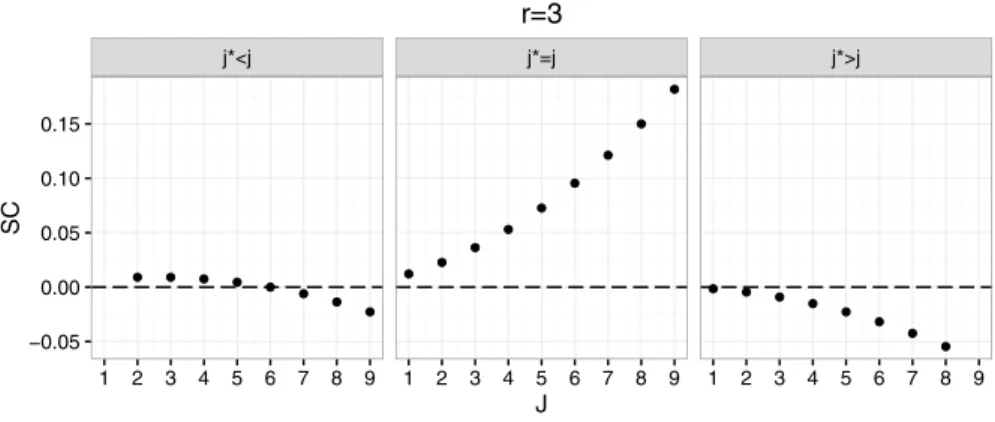
Figures 1, 2 and 3 illustrate the NPI-SC for the event X(r)∈Ij , for r=1, 2, 3 , j=1,…, 9 and j∗<j , j∗=j and j∗>j . These figures illustrate that SCP(X(r)∈Ij)(x, y)
is symmetric, i.e. SCP(X(r)∈Ij)(x, y) =SCP(X(m+1−r)∈In+2−j)(x, y), so such as
SCP(X(1)∈I9)(x, y) =SCP(X(3)∈I1)(x, y) . For all r, the NPI-SC for X(r)∈Ij is unimodal
in j.
To illustrate the c-breakdown point 𝜆∗
c for the event X(r) ∈Ij , we choose c=0.05
and plot the absolute value of SCP(X(
r)∈Ij)(x, y1,…, yl) as function of l, where l is the
j*<j j*=j j*>j −0.05 0.00 0.05 0.10 0.15 1 2 3 4 5 6 7 8 9 1 2 3 4 5 6 7 8 9 1 2 3 4 5 6 7 8 9 J SC r=3 Fig. 3 SCP(X
(3)∈Ij)(x,y) for n=8 and m=3
Table 3 SCP(X(r)∈Ij)(x,y1,…,yl) for m=3 r l j=1 l j=2 l j=3 l j=4 l j=5 1 2 0.0420 4 0.0468 7 0.0410 7 0.0158 7 0.0047 3 0.0584 5 0.0557 8 0.0459 8 0.0189 8 0.0030 2 7 0.0349 4 0.0442 3 0.0449 3 0.0466 3 0.0416 8 0.0370 5 0.0505 4 0.0547 4 0.0575 4 0.0526 3 7 0.0048 7 0.0145 7 0.0290 7 0.0484 3 0.0497 8 0.0050 8 0.0151 8 0.0302 8 0.0503 4 0.0579 Table 4 SCP(X(r)∈Ij)(x,y1,…,yl) for m=3 r l j=6 l j=7 l j=8 l j=9 1 7 0.0203 7 0.0310 7 0.0370 7 0.0381 8 0.0199 8 0.0317 8 0.0386 8 0.0404 2 5 0.0490 7 0.0415 7 0.0087 7 0.0337 6 0.0572 8 0.0478 8 0.0144 8 0.0290 3 1 0.0318 1 0.0424 1 0.0545 1 0.0682 2 0.0538 2 0.0718 2 0.0923 2 0.1154
number of the contaminated values that have been added to the data set of size
n=8 . These are given in Tables 3 and 4 for r=1, 2, 3 . For r=1 and j≥3 , the probability for the event X(1)∈Ij does not break down, whereas for j=1 , 𝜆∗ 0.05(P(X(1) ∈I1),(x, y9, y10, y11)) = 3 11=0.2727 and for j=2 , 𝜆∗ 0.05(P(X(1) ∈I2),(x, y9,…, y13)) = 5
13 =0.3846 . These tables present the absolute
value of the NPI-SC for X(2)∈Ij , where for j=3, 4, 5 the NPI-BP is 4
12=0.3333 , for j=2 it is 5
13=0.3846 and for j=6 it is
6
14=0.4286 . The probability for the
event X(2) ∈Ij for j=1, 7, 8, 9, does not break down as
SCP(X(2)∈Ij)(x, y1,…, y8) <0.05 . For r=3 , and j=4 ,
𝜆∗
0.05(P(X(3) ∈Ij),(x, y9,…, y16)) = 8
16=0.5 , whereas as j increases the NPI-BP decreases, such that for j=8, 9 , 𝜆∗0.05(P(X(3)∈Ij),(x, y9)) =1∕9.
6 Robustness of the Median and Mean of the Future Observations In the classical robustness literature there has been quite a lot of emphasis on robust estimation of a location parameter, where typically they compare the robustness of the mean and the median. In this section, we illustrate the use of the robustness concepts for NPI, namely NPI-SC and NP-BP, by considering events involving the median and the mean of the m future observations.
6.1 Median of the m Future Observations
We first examine how contamination in the data affects NPI for an event involving the median of the m future observations, for odd-valued m. We consider the NPI-SC for the lower and upper probabilities for the event Mm<z . We wish to examine the
effect on [P, P](Mm<z) of adding a contaminant 𝛿 to one of the observations xj with
j=1,…, n . Let z∈Ik= (xk−1, xk) , if we add 𝛿 to xj this becomes ̃xl=xj+ 𝛿 , where
𝛿∈ℝ . The NPI-SC for event Mm<z is
SCP(Mm<z)(x(j,𝛿)) = ⎧ ⎪ ⎨ ⎪ ⎩ 0 if xj>z and x̃l>z 0 if xj<z and x̃l<z P(Mm∈Ik) if xj>z and x̃l<z −P(Mm∈Ik−1) if xj<z and x̃l>z SCP(M m<z)(x(j,𝛿)) = ⎧ ⎪ ⎨ ⎪ ⎩ 0 if xj>z and x̃l>z 0 if xj<z and x̃l<z P(Mm∈Ik+1) if xj>z and x̃l<z −P(Mm∈Ik) if xj<z and x̃l>z
The NPI-SC for lower and upper probabilities for the event Mm<z is a step
func-tion, with the step occurring when the contamination value changes the number of intervals to the right of z.
Next we consider the NPI-SC for the lower and upper probability for the event that Mm∈ (z1, z2) . Let z1∈Ik and z2∈Id where k≤d . If we add 𝛿 to one of the
data observations, i.e. xj is replaced by x̃l , then there are three possible situations.
The effect of adding 𝛿 to xj is to change the value of the NPI lower and upper prob-abilities for the event Mm∈ (z1, z2) , by an amount NPI-SC as specified for each case below. First, if xj<z1 Secondly, if xj>z2 Thirdly, if xj∈ (z1, z2) (29) SCP(Mm∈(z1,z2))(x(j,𝛿)) =Px(j,𝛿)(Mm∈ (z1, z2)) −Px(Mm∈ (z1, z2)) = ⎧ ⎪ ⎨ ⎪ ⎩ 0 if x̃l<z1 P(Mm∈Ik) if x̃l∈ (z1, z2) P(Mm∈Ik) −P(Mm∈Id−1) if x̃l>z2 (30) SCP(M m∈(z1,z2))(x(j,𝛿)) =Px(j,𝛿)(Mm∈ (z1, z2)) −Px(Mm∈ (z1, z2)) = ⎧ ⎪ ⎨ ⎪ ⎩ 0 if x̃l<z1 P(Mm∈Ik−1) if x̃l∈ (z1, z2) P(Mm∈Ik−1) −P(Mm∈Id) if x̃l>z2 SCP(Mm∈(z1,z2))(x(j,𝛿)) = ⎧ ⎪ ⎨ ⎪ ⎩ 0 if x̃l>z2 P(Mm∈Id) if x̃l∈ (z1, z2) P(Mm∈Id) −P(Mm∈Ik+1) if x̃l<z1 SCP(M m∈(z1,z2))(x(j,𝛿)) = ⎧ ⎪ ⎨ ⎪ ⎩ 0 if x̃l>z2 P(Mm∈Id+1) if x̃l∈ (z1, z2) P(Mm∈Id+1) −P(Mm∈Ik) if x̃l<z1 (31) SCP(Mm∈(z1,z2))(x(j,𝛿)) = ⎧ ⎪ ⎨ ⎪ ⎩ 0 if x̃l∈ (z1, z2) −P(Mm∈Id−1) if x̃l>z2 −P(Mm∈Ik+1) if x̃l<z1
So, when the data are contaminated and that contamination does not affect the num-ber of intervals in (z1, z2) then there is no effect on this inference at all, which is an attractive property. But this is not the same if m is even , which leads to more com-plicated analysis due to the definition of Mm as the overage of two observation. For study of the robustness of Mm for even-valued m we refer to the PhD thesis of [1].
The c-breakdown point for the NPI lower and upper probabilities for the event
Mm>z and Mm>(z1, z2) , where z, z2∈Ik and m is odd, are similar as presented in
Sect. 5, if we replace X(r) by Mm in Eq. (27). The NPI lower and upper probabilities
for such an event depend only on the number of observations that are greater than z
or within (z1, z2) , so in the sample of n observations, only n−k+2 or more outliers
can cause these probabilities to change.
6.2 Mean of the m Future Observations
We consider the NPI-SC for the mean of the m future observations. It is well known that the mean of the population in classical statistics is more sensitive than the median to a single contamination in the data [22]. We investigate the robustness of inferences involving the mean of the m future observations. The lower and upper bounds for the mean of the m future observations given the ordering Oi , as given in Eqs. (7) and (8), depend on the value of sij . The NPI-SC for the lower and upper
bounds of the 𝜇mi , if xj becomes xj+ 𝛿 = ̃xl , for 𝛿 >0 and l>j or for 𝛿 <0 and l<j ,
are
As a special case, if l=j , i.e. xj+ 𝛿 did not shift from its rank among the observa-tions, so xj−1<xj+ 𝛿 <xj+1 , then the NPI-SC for 𝜇im and 𝜇im are
1 ms i j+1𝛿 and 1 ms i j𝛿 ,
respectively. If the value of sij=sij+1=0 then there is no influence at all on the lower and upper 𝜇mi , whereas if sij=m and sij+1 =m then NPI-SC of the lower or the upper (32) SCP(M m∈(z1,z2))(x(j,𝛿)) = ⎧ ⎪ ⎨ ⎪ ⎩ 0 if x̃l∈ (z1, z2) −P(Mm∈Id) if x̃l>z2 −P(Mm∈Ik) if x̃l<z1 (33) SC𝜇i m(x(j,𝛿)) = 1 m [ l ∑ k=j sik+1[̃xk−xk] ] (34) SC𝜇i m (x(j,𝛿)) = 1 m [ l ∑ k=j sik[̃xk−xk] ]
bound for 𝜇i
m , will exceed any bound for 𝛿 large or small enough. The NPI-SC for 𝜇m≥z , if xj becomes xj+ 𝛿 = ̃xl and 𝛿∈ℝ , is
The NPI-SC of the lower and upper probabilities for the event 𝜇m∈ (z1, z2)) , are
and
These NPI-SC will be illustrated in Example 2 in Sect. 6.3.
The c-breakdown points of the lower and upper bounds of 𝜇i m , are 1 n for si l+1≠0 and s i
l≠0 respectively. This is because if we hold x1,…, xn−1 fixed and let xn go to infinity then 𝜇i
m also goes to infinity if s i
l+1≠0 or s i
l≠0 , correspond-ing to 𝜇i
m and 𝜇mi . However, when we consider inference involving the mean, we will not let xn go to infinity, as we have assumed bounds for the data observations
SCP(𝜇m≥z)(x(j,𝛿)) = ⎛ ⎜ ⎜ ⎝ n+m n ⎞ ⎟ ⎟ ⎠ � i=1 P(Oi)�1 � 𝜇im(x(j,𝛿))≥z � −1 � 𝜇mi(x)≥z �� SCP(𝜇 m≥z)(x(j,𝛿)) = ⎛ ⎜ ⎜ ⎝ n+m n ⎞ ⎟ ⎟ ⎠ � i=1 P(Oi)�1 � 𝜇i m(x(j,𝛿))≥z � −1 � 𝜇i m(x)≥z �� SCp(𝜇m∈(z1,z2))(x(j,𝛿)) =Px(j,𝛿)(𝜇m∈ (z1, z2)) −Px(𝜇m∈ (z1, z2)) = ⎛ ⎜ ⎜ ⎝ n+m n ⎞ ⎟ ⎟ ⎠ � i=1 P(Oi) � 1 � z1≤𝜇im(x(j,𝛿))≤𝜇i m(x(j,𝛿))≤z2 � −1 � z1≤𝜇mi(x)≤𝜇i m(x)≤z2 �� (35) SCp(𝜇 m∈(z1,z2))(x(j,𝛿)) =Px(j,𝛿)(𝜇m ∈ (z1, z2)) −Px(𝜇m ∈ (z1, z2)) = ⎛ ⎜ ⎜ ⎝ n+m n ⎞ ⎟ ⎟ ⎠ � i=1 P(Oi)�1 � (𝜇i m(x(j,𝛿)),𝜇mi(x(j,𝛿))) ∩ (z1, z2)≠� � −1 � (𝜇i m(x),𝜇mi(x)) ∩ (z1, z2)≠� ��
L<x1<⋯<xn<R . So 𝜆∗c(𝜇 i
m, x(𝛿, j1,…, jl)) may not be equal to
1
n . This will be illustrated in Example 2 in Sect. 6.3.
6.3 Comparison of Robustness of the Median and the Mean of the Future Observations
A main topic in the classical theory of robustness is comparison of the robustness of the mean and the median. The mean is typically very sensitive to small changes in the data, whereas the median is more robust. In our case the inferences that involve the median of the m future observations depend on the event of interest, for example, the lower and upper probabilities for the event Mm>z might slightly be affected
if the contaminant changes the number of observations that are less than z, and its effect is a step function, as will be illustrated in Example 2. The 0-breakdown point for Mm>z , where z∈ (xk−1, xk) , is
n−k+2
n , so the value of NPI-BP for the median decreases as the value of k increases. If we replace xj by ̃xl , then the inferences of
events involving the mean of the m future observations might be affected by a small change in the data, if sil , the number of future observations in Il given the ordering
Oi , is not equal to zero. Example 2 illustrates the NPI-SC and NPI-BP for inferences
involving the mean and the median of the m future observations.
Example 2 To illustrate the NPI-SC for different inferences involving the
median and mean of the m=3 future observations, we consider the data set x= {−9,−7, 0, 2, 5, 7, 10, 16} so n=8 , and the contaminated sample x(2,𝛿) , where we add 𝛿 to x2= −7 and 𝛿∈ℝ . When we consider the mean of the 3 future observa-tions, we set x0=L= −17 and x9=R=18 as bounds for the observations.
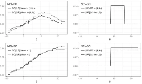
Figure 4 shows the NPI-SC for the NPI lower and upper probabilities for the events 𝜇3 ≥1 , 𝜇3 ∈ (1, 9) , M3≥1 and M3∈ (1, 9) given x , and the contaminated sample x(2,𝛿) . Note that the NPI lower probability for such an event of interest in these figures is denoted by LP, and the NPI upper probability by UP. The NPI-SC for 𝜇3≥1 increases as the value of −7+ 𝛿 increases, and the maximum NPI-SC
for the lower and upper probabilities for 𝜇3≥1 are 0.1576 and 0.1333 respectively, which occur at −7+ 𝛿 =16 which is the largest contaminated value, as 𝛿 can not go
to 25 as we set R=18 as upper bound for the observations. The inferences involving
the median of the m=3 future observations depend on the ranks of the observa-tions, which are only affected if the number of the observations that are greater than 1, or in (1, 9), changes, so NPI-SC is a step function. The NPI-SC for the NPI lower and upper probabilities for M3≥1 are 0.1454 and 0.1273 respectively, which occur at 𝛿 >8 . So it is less than NPI-SC for 𝜇3 ≥1 . The NPI-SC for the event 𝜇3 ∈ (1, 9) increases till 𝛿≥12.3 then for 𝛿 >12.3 it decreases to be close to zero. The maxi-mum NPI-SC for the lower and upper probabilities for 𝜇3∈ (1, 9) are 0.0667 and 0.0909 respectively, and it occurred at 𝛿=10.8 . The maximum NPI-SC for the NPI lower and upper probabilities for M3∈ (1, 9) are 0.1454 and 0.1273 respectively, so it is greater than NPI-SC for 𝜇3∈ (1, 9) . Table 5 shows that for 𝛿 <7 and 𝛿 >19 ,
the median. In contrast, for 8< 𝛿≤15.3 the inferences involving the mean are more
robust.
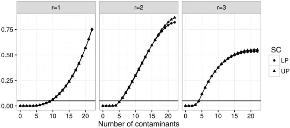
To illustrate the c-breakdown point, we consider NPI-SC as function of the num-ber of contaminants present in the data, starting by replacing x8 by x8+ 𝛿8 , then x8 and x7 by x8+ 𝛿8 and x7+ 𝛿7 , and so on, until all observations have been
contami-nated by {𝛿1,…,𝛿8} = {18.5, 17.5, 11, 9.5, 7, 5.5, 3, 1} . Figure 5 shows the NPI-SC
for the lower and upper probabilities for 𝜇3 ≥1 and M3≥1) , as functions of the
number of the observations that have been contaminated by adding different values of 𝛿 to them. The results clearly show that when we contaminate up to 5
observa-tions, which are 2, 5, 7, 10, 16 in the data, to become 11.5, 12, 12.5, 13, 17, the inference involving the median X(2)≥1 is not affected at all, whereas the inference
involving the mean of the future observations is affected. If we choose c=0.15 , then the c-breakdown points for the lower and upper probabilities for M3≥1 and for the upper probability for 𝜇3≥1 , are all equal to 0.875, so breakdown occurs when we change 7 observations out of 8, whereas the c-breakdown point for the NPI lower probability for 𝜇3≥1 is 0.625, so breakdown occurs if 5 out of 8 observations are contaminated.
7 Robustness of Other Inferences
In this section we consider the use of the presented tools for robustness, namely NPI-SC and NPI-BP, for pairwise comparisons and for reproducibility of tests, as presented by [8, 9]. −0.07 0.00 0.07 0.14 −10 0 10 20 δ NPI−SC SC([LP](Mean in (1,9) )) SC([UP](Mean in (1,9))) −0.07 0.00 0.07 0.14 −10 0 10 20 δ NPI−SC SC([LP](Mean > 1 ) SC([UP](Mean >1) −0.07 0.00 0.07 0.14 −10 0 10 20 δ NPI−SC [LP](M3 in (1,9) ) [UP](M3 in (1,9)) −0.07 0.00 0.07 0.14 −10 0 10 20 δ NPI−SC [LP](M3 in (1,9) ) [UP](M3 in (1,9))
7.1 Pairwise Comparisons
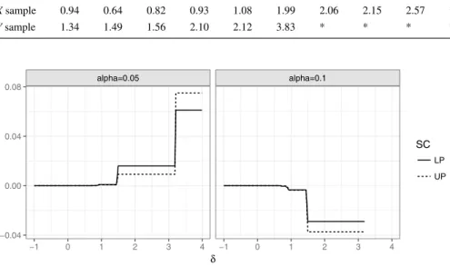
We investigate the robustness of one of the applications of NPI for future order sta-tistics for statistical inference problems, as presented by [9]. Suppose that we have two independent groups of real-valued observations, X and Y and their ordered observed values are x1<x2 <⋯<xnx and y1 <y2<⋯<yny . For ease of notation, let x0=y0= −∞ and xn x+1=yny+1= ∞ . Let I x jx = (xjx−1, xjx) and I y jy = (yjy−1, yjy) . We focus attention on m≥1 future observations from each group, Xn
x+i and Yny+i for i=1,…, m . We wish to compare the r-th future order statistics from these two groups by considering the event X(r)<Y(r) , for which the NPI lower and upper prob-abilities, based on the A(n
x) and A(ny) assumptions per group, are derived by
0.00 0.05 0.10 0.15 0.20 0.25 0.30 0.35 0 1 2 3 4 5 6 7 8 Number of contaminants SC([LP](Median > 1)) SC([UP](Median > 1)) 0.00 0.05 0.10 0.15 0.20 0.25 0.30 0.35 0 1 2 3 4 5 6 7 8 Number of contaminants SC([LP](Mean > 1)) SC([UP](Mean > 1))
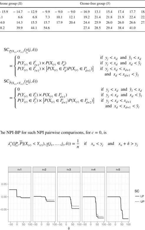
The NPI-SC of the lower and upper probabilities for the event that X(r) <Y(r) , if we replace yj by yj+ 𝛿 , which we denote by ỹl , are
P(X(r)<Y(r)) = n∑x+1 jx=1 ny+1 ∑ jy=1 𝟏{xj x <yjy−1 } P(X(r)∈Ix jx ) P(Y(r)∈Iyj y ) P(X(r)<Y(r)) = n∑x+1 jx=1 n∑y+1 jy=1 𝟏{xj x−1<yjy } P(X(r)∈Ijx x ) P(Y(r)∈Iyj y ) Table 5 SCI(x(2,𝛿)) for m=3 𝜇3≥1 M3≥1 𝜇3∈ (1, 9) M3∈ (1, 9) 𝛿 SCP SCP SCP SCP SCP SCP SCP SCP − 9 − 0.0545 − 0.0667 0 0 − 0.0485 − 0.0667 0 0 − 7.41 − 0.0485 − 0.0545 0 0 − 0.0424 − 0.0545 0 0 − 5.82 − 0.0364 − 0.0424 0 0 − 0.0303 − 0.0424 0 0 − 4.23 − 0.0303 − 0.0364 0 0 − 0.0242 − 0.0364 0 0 − 2.64 − 0.0242 − 0.0303 0 0 − 0.0182 − 0.0303 0 0 − 1.05 − 0.0121 − 0.0182 0 0 − 0.0121 − 0.0182 0 0 0.54 0.0061 0.0061 0 0 0.0000 0.0061 0 0 2.13 0.0121 0.0182 0 0 0.0000 0.0121 0 0 3.72 0.0364 0.0424 0 0 0.0242 0.0364 0 0 5.31 0.0485 0.0545 0 0 0.0364 0.0485 0 0 6.9 0.0606 0.0667 0 0 0.0424 0.0606 0 0 8.49 0.0788 0.0848 0.1455 0.1273 0.0545 0.0727 0.1455 0.1273 10.08 0.0970 0.1030 0.1455 0.1273 0.0667 0.0909 0.1455 0.1273 11.67 0.1030 0.1030 0.1455 0.1273 0.0545 0.0848 0.1455 0.1273 12.9 0.1091 0.1091 0.1455 0.1273 0.0545 0.0848 0.1455 0.1273 13.26 0.1152 0.1152 0.1455 0.1273 0.0545 0.0848 0.1455 0.1273 14.85 0.1212 0.1212 0.1455 0.1273 0.0485 0.0848 0.1455 0.1273 15.3 0.1212 0.1212 0.1455 0.1273 0.0485 0.0848 0.1455 0.1273 16.44 0.1212 0.1212 0.1455 0.1273 0.0242 0.0667 0.0000 − 0.0000 18.03 0.1394 0.1273 0.1455 0.1273 0.0182 0.0485 0.0000 − 0.0000 19.62 0.1455 0.1333 0.1455 0.1273 0.0121 0.0424 0.0000 − 0.0000 21.21 0.1515 0.1333 0.1455 0.1273 0.0061 0.0303 0.0000 − 0.0000 22.8 0.1576 0.1333 0.1455 0.1273 0.0000 0.0182 0.0000 − 0.0000 24.39 0.1576 0.1333 0.1455 0.1273 − 0.0121 0.0061 0.0000 − 0.0000