A comparison of cancer classification methods based on microarray data.

(1)

A Comparison of Cancer

Classification Methods Based

on Microarray Data

Mohanad Mohammed April, 2018

(2)

A Comparison of Cancer Classification Methods

Based on Microarray Data

by

Mohanad Mohammed

A thesis submitted to the University of KwaZulu-Natal

in fulfilment of the requirements for the degree of

MASTER OF SCIENCE in

STATISTICS

Thesis Supervisor: Henry Mwambi Thesis Co-supervisor: Bernard Omolo

UNIVERSITY OF KWAZULU-NATAL

SCHOOL OFMATHEMATICS, STATISTICS ANDCOMPUTERSCIENCE

(3)

Declaration - Plagiarism

I, Mohanad Mohammed, declare that

1. The research reported in this thesis, except where otherwise indicated, is my original research.

2. This thesis has not been submitted for any degree or examination at any other university.

3. This thesis does not contain other persons’ data, pictures, graphs or other in-formation, unless specifically acknowlegded as being sourced from other per-sons.

4. This thesis does not contain other persons’ writing, unless specifically acknowl-edged as being sourced from other researchers. Where other written sources have been quoted, then

(a) their words have been re-written but the general information attributed to them has been referenced, or

(b) where their exact words have been used, then their writing has been placed in italics and referenced.

5. This thesis does not contain text, graphics or tables copied and pasted from the internet, unless specifically acknowledged, and the source being detailed in the thesis and in the reference sections.

Mohanad Mohammed (Student) Date

Henry Mwambi (Supervisor) Date

(4)

Disclaimer

This document describes work undertaken as a Masters programme of study at the University of KwaZulu-Natal (UKZN). All views and opinions expressed therein remain the sole responsibility of the author, and do not necessarily represent those of the institution.

(5)

Abstract

Cancer is among the leading causes of death in both developed and developing countries. Through gene expression profiling of tumors, the accuracy of cancer clas-sification has been enhanced, leading to correct diagnoses and the application of effective therapies. Here, we discuss a comparative review of the binary class pre-dictive ability of seven classification methods (support vector machines, with the radial basis kernel (SVM(RK)), linear kernel (SVM(LK)) and the polynomial kernel (SVM(PK)), artificial neural networks (ANN), random forests (RF),k-nearest neigh-bor (KNN), and naive Bayes (NB)), using publicly-available gene expression data from cancer research. Results indicate that NB outperformed the other methods in terms of the accuracy, sensitivity, specificity, kappa coefficient, area under the curve (AUC), and balanced error rate (BER) of the binary classifier. Thus, overall the Naive Bayes (NB) approach turned out to be the best classifier with our datasets.

(6)

Dedication

This dissertation is dedicated to my supervisors, my parents, my brothers, my sisters, teachers, and friends

who have always taught me how to see the vitality in myself, conquer fears and overcome challenges.

(7)

Acknowledgements

In the name of the Almighty God, most Gracious, most Merciful. Praise be to God, the Cherisher and Sustainer of the world.

I am highly grateful to the Almighty God for His unmeasurable Mercies that saw me through my studies. It is such a great honour for me and humbling at the same time because it has been a long journey characterized by long hours of hard work and sacrifice. It is with pleasure and gratitude to acknowledge those who rendered assistance through the lengthy process of my study. I sincerely appreciate all the big and small contributions from everybody who either directly or indirectly helped make my studies less stressful and a success.

I am specifically grateful to my supervisors,Prof. Henry MwambiandProf. Bernard Omolofor their presence, inspiration, patience, dedication and their powerful guid-ance and help. I again thank them for their availability and readiness to read and correct all the many errors in my work, as well as the financial support. Much thanks for their quick responses whenever I consulted. Their help in and outside the re-search has been immense. I am deeply grateful for their willingness to work with me. Thank you both for sharing your enormous statistical knowledge with me. I would also like to thankMiss Christel Bernardfor ensuring I have a comfortable working place environment and for her patience on my many questions.

Special thanks to all my colleagues and friends inside and outside South Africa, es-pecially I would like thankDr. Murtada Khalafallahfor his moral and enthusiastic support, who encouraged me when I first started working on this project.

Many thanks go toMs Justine Nasejje for her help, encouragement and assisting on some methods relevant to my research.

(8)

the important things in life and have supported all my endeavours, for their uncon-ditional love, encouragement, patience for being away when they needed me the most.

I am grateful and thankful to my brothers and sisters,Modather,Mogtba,Zahrra, andTanzeelfor their caring of my parents. Many thanks to the rest of my extended family for your moral support.

Last, but not least, thanks to everyone who his or her names may not appear here, but I won’t forget their help. May the Almighty bless them all.

I would like to express my profound gratitude to the School of Mathematics, Statis-tics, and Computer Science, College of Agriculture, Engineering, and Science, Uni-versity of KwaZulu-Natal, South Africa and the Ministry of Higher Education & Scientific Research represented in Faculty of Mathematical and Computer Sciences, University of Gezira, Sudan for their support and financial help to complete this Masters project successfully.

Funding

This work was supported through the DELTAS Africa Initiative. The DELTAS Africa Initiative is an independent funding scheme of the African Academy of Sciences (AAS) Alliance for Accelerating Excellence in Science in Africa (AESA) and sup-ported by the New Partnership for Africa’s Development Planning and Coordi-nating Agency (NEPAD Agency) with funding from the Wellcome Trust [ grant 107754/Z/15 /Z- DELTAS Africa Sub-Saharan Africa Consortium for Advanced Biostatistics (SSA CAB) programme ] and the UK government. The views expressed in this publication are those of the author(s) and not necessarily those of AAS, NEPAD Agency, Wellcome Trust or the UK government.

(9)

Chapter 2: Data description 10 2.1 Dataset 1: GSE5851 . . . 11 2.2 Dataset 2: GSE7670 . . . 11 2.3 Dataset 3: GSE8401 . . . 11 2.4 Dataset 4: GSE10072 . . . 11 2.5 Dataset 5: GSE10245 . . . 11 2.6 Dataset 6: GSE23988 . . . 12 2.7 Dataset 7: GSE25136 . . . 12 2.8 Dataset 8: GSE32962 . . . 12 2.9 Dataset 9: GSE35896 . . . 12 2.10 Dataset 10: GSE103091 . . . 13 Chapter 3: Methodology 14

(10)

CONTENTS

3.1 Support Vector Machines (SVM) . . . 14

3.1.1 Kernel Function . . . 16

3.2 Artificial Neural Networks (ANN) . . . 17

3.3 Naive Bayes (NB) . . . 19

3.4 Random Forests (RF) . . . 20

3.5 k-Nearest Neighbor (KNN) . . . 21

3.6 Performance Measures . . . 22

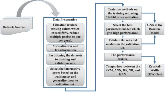
Chapter 4: Application and Results 24 4.1 Data Source . . . 25

4.2 Data Preparation . . . 25

4.2.1 Filtration . . . 25

4.2.2 Normalization and Transformation . . . 25

4.2.3 Datasets Partitioning . . . 25

4.2.4 Features (Genes) Selection . . . 26

4.3 Model Training . . . 26

4.4 Model Validation . . . 26

4.5 Baseline Model . . . 27

4.6 Kruskal-Wallis (KW) Test . . . 27

4.7 Results . . . 28

4.7.1 Training Results of the Methods on the GSE8401 . . . 28

4.7.2 GSE8401: . . . 34 4.7.3 GSE23988: . . . 35 4.7.4 GSE7670: . . . 36 4.7.5 GSE10072: . . . 38 4.7.6 GSE10245: . . . 39 4.7.7 GSE25136: . . . 41 4.7.8 GSE35896: . . . 42 4.7.9 GSE103091: . . . 44 4.7.10 GSE5851: . . . 45 4.7.11 GSE32962: . . . 47

Chapter 5: Discussion and Conclusion 50

References 58

Appendix A 59

(11)

CONTENTS

(12)

List of Figures

Figure1.1 Work flow of the Affymetrix microarray experiment. . . 4 Figure3.1 (a) Original data in the input space. (b) Mapped data in the feature space.16 Figure3.2 Multi-layer neural networks architecture. . . 19 Figure3.3 k-nearest neighbor approach. . . 22 Figure4.1 Flow diagram of the data processing stages until final model comparison

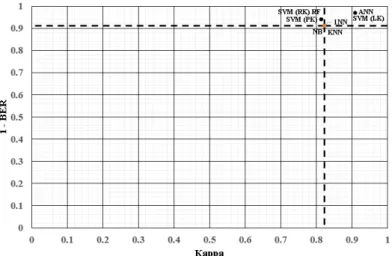
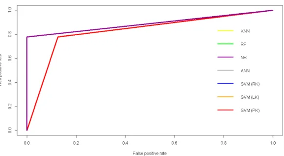
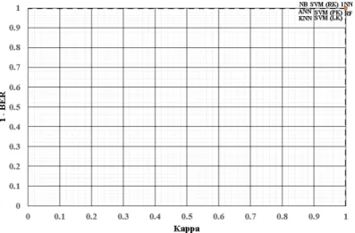
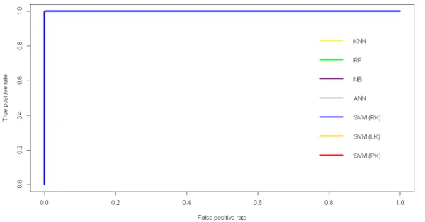
and performance. . . 24 Figure4.2 ROC curves for all the methods applied to the GSE8401 dataset. . . 34 Figure4.3 Plot of 1 - BER against kappa for the GSE8401 dataset. The dashed lines

represent the values of the baseline model. The best performing models are to the top-right. . . 35 Figure4.4 ROC curves for all the methods applied to the GSE23988 dataset. . . 36 Figure4.5 Plot of 1 - BER against kappa for the GSE23988 dataset. The dashed lines

represent the values of the baseline model. . . 38 Figure4.8 ROC curves for all the methods applied to the GSE10072 dataset. . . 39 Figure4.9 Plot of 1 - BER against kappa for the GSE10072 dataset. The dashed lines

represent the values of the baseline model. . . 39 Figure4.10 ROC curves for all the methods applied to the GSE10245 dataset. . . 40 Figure4.11 Plot of 1 - BER against kappa for the GSE10245 dataset. The dashed lines

(13)

LIST OF FIGURES

Figure4.12 ROC curves for all the methods applied to the GSE25136 dataset. . . 42 Figure4.13 Plot of 1 - BER against kappa for the GSE25136 dataset. The dashed lines

represent the values of the baseline model. The best performing models are to the top-right. . . 48

(14)

List of Tables

Table2.1 Summary of the gene expression datasets used in the study. Here Pos and Neg represents positive and negative, respectivlely. GSE(GEO Sample), GPL(GEO

Platform). . . 10

Table3.1 Kernel Functions.. . . 16

Table3.2 Structure of the confusion matrix. . . 22

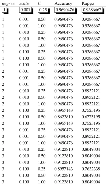
Table4.1 Tuning Parameter Results of KNN for GSE8401 . . . 29

Table4.2 Confusion Matrix of KNN on GSE8401 Validation Set. . . 29

Table4.3 Tuning Parameter Results of NB for GSE8401 . . . 29

Table4.4 Confusion Matrix of NB on GSE8401 Validation Set . . . 29

Table4.5 Tuning Parameter Results of RF for GSE8401 . . . 30

Table4.6 Confusion Matrix of RF on GSE8401 Validation Set . . . 30

Table4.7 Tuning Parameter Results of SVM(RK) for GSE8401 . . . 30

Table4.8 Confusion Matrix of SVM(RK) on GSE8401 Validation Set . . . 31

Table4.9 Tuning Parameter Results of SVM(LK) for GSE8401 . . . 31

Table4.10 Confusion Matrix of SVM(LK) on GSE8401 Validation Set . . . 31

Table4.11 Tuning Parameter Results of SVM(PK) for GSE8401 . . . 32

Table4.12 Confusion Matrix of SVM(PK) on GSE8401 Validation Set . . . 33

Table4.13 Tuning Parameter Results of ANN for GSE8401 . . . 33

Table4.14 Confusion Matrix of ANN on GSE8401 Validation Set. . . 33

Table4.15 Summary accuracy measures for all the candidate methods using the GSE8401 data set. Accuracy and Kappa values were obtained for both the validation and training (in bracket) sets. . . 34

(15)

LIST OF TABLES

Table4.18 Summary accuracy measures for all the candidate methods using the GSE10072 data set. Accuracy and Kappa values were obtained for both the validation and

training (in bracket) sets. . . 38

Table4.25 Average accuracies of the seven classification methods based on the ten val-idation datasets. . . 49

TableB.1 Tuning Parameter Results of KNN for GSE23988 . . . 66

TableB.2 Confusion Matrix of KNN on GSE23988 Validation Set . . . 67

TableB.3 Tuning Parameter Results of NB for GSE23988 . . . 67

TableB.4 Confusion Matrix of NB on GSE23988 Validation Set . . . 67

TableB.5 Tuning Parameter Results of RF for GSE23988 . . . 67

TableB.6 Confusion Matrix of RF on GSE23988 Validation Set . . . 68

TableB.7 Tuning Parameter Results of SVM(RK) for GSE23988 . . . 68

TableB.8 Confusion Matrix of SVM(RK) on GSE23988 Validation Set . . . 68

TableB.9 Tuning Parameter Results of SVM(LK) for GSE23988 . . . 68

TableB.10 Confusion Matrix of SVM(LK) on GSE23988 Validation Set. . . 68

TableB.11 Tuning Parameter Results of SVM(PK) for GSE23988 . . . 69

TableB.12 Confusion Matrix of SVM(PK) on GSE23988 Validation Set. . . 70

TableB.13 Tuning Parameter Results of ANN for GSE23988 . . . 70

TableB.14 Confusion Matrix of ANN on GSE23988 Validation Set . . . 70

(16)

LIST OF TABLES

TableB.16 Confusion Matrix of KNN on GSE7670 Validation Set. . . 71

TableB.24 Confusion Matrix of SVM(LK) on GSE7670 Validation Set . . . 73

TableB.26 Confusion Matrix of SVM(PK) on GSE7670 Validation Set . . . 75

TableB.28 Confusion Matrix of ANN on GSE7670 Validation Set. . . 75

TableB.34 Confusion Matrix of on GSE10072 Validation Set . . . 77

TableB.36 Confusion Matrix SVM(RK) on GSE10072 Validation Set . . . 77

(17)

LIST OF TABLES

TableB.64 Confusion Matrix of SVM(RK) . . . 87

TableB.88 Confusion Matrix of NB on GSE103091 Validation Set. . . 96

(18)

LIST OF TABLES

TableB.116 Confusion Matrix of NB on GSE32962 Validation Set. . . 106

(19)

(20)

LIST OF TABLES

Abbreviations

SVM Support Vector Machines ANN Artificial Neural Networks

SVM(RK) Support Vector Machines (Radial basis Kernel) SVM(LK) Support Vector Machines (Linear Kernel) SVM(PK) Support Vector Machines (Polynomial Kernel)

RF Random Forests

KNN k-Nearest Neighbor

NB Naive Bayes

AUC Area Under the Curve BER Balanced Error Rate ROC Receiver Operating Curve DNA Deoxyribonucleic Acid RNA Ribonucleic Acid

LDA Linear Discriminant Analysis DT Decision Trees

MLP Multi-Layer Perceptrons

DLBCL Diffuse Large B-cell Lymphoma GCB-like Germinal Centre B-like DLBCL AB-like Activated B-like DLBCL

QDA Quadratic Discriminant Analysis KPCA Kernel Principal Component Analysis LR Logistic Regression

NC nearest centroid

ALL Acute Lymphoblastic Leukemia AML Acute Myleloid Leukemia GEO Gene Expression Omnibus GPL GEO Platform accession number GSE GEO Sample accession number

Prim primary

Met metastatic

NSCLC Non-Small Cell Lung Cancer

AC Adenocarcinoma

SCC Squamous Cell Carcinoma

Rec Recurrence NonRec Non-Recurence MetFree metastatis-free Sens sensitive Resist resistant TP True Positive FP False Positive TN True Negative FN False Negative xvi

(21)

Chapter 1

Introduction

1.1 Background

Classification plays an essential role in understanding diseases. It is a form of data analysis that uses statistical and mathematical methods or models to classify observations or samples into different distinct categories. To classify the data, two steps are followed; the learning step and the classification step. The learning step is where the classification model is constructed based on training data. The classi-fication step is where the constructed model is used to predict classes for a given data. Predictive modeling is a statistical method used to build predictive models to separate and classify new data points. There are two types of learning approaches, namely, the supervised and unsupervised learning. Supervised learning is where the class labels of each training observation or sample is provided. In contrast, un-supervised learning (or clustering) is where the class label of each training data is unknown, and the number of classes to be learned may not be known in advance (Han et al.,2011). Disease classification is very important for early detection, treat-ment, containment and other etiological and intervention applications. This ulti-mately helps to improve health and reduce negative outcomes such as death.

Recent global public health research shows an epidemiological transition from infectious to non-communicable diseases, the latter including different types of can-cers. The incidence and prevalence of cancer is on the increase worldwide, both in the developing and developed countries (Olsen,2015;Morhason-Bello et al.,2013).

Cancer is a disease in which cells in particular tissues in the body undergo uncon-trolled division. This situation results in a malignant growth or tumor. Cancerous cells very often invade and destroy surrounding healthy tissues and organs. When there is no intervention, the body cells continue to divide and spread into adjacent tissues. The tumor can occur at any part of the human cells. Normally, the human cells grow and separate to make new cells as needed by the body to replace the old

(22)

1.1. Background

cells. When cancer occurs, this process does not go as it is supposed to be, rather the cells abnormally split without constraint and form outgrowths in the body called tumors. The tumors can spread or attack the surrounding tissues, which in this case, these are calledmalignant tumors. Furthermore, some growth cells can move to a dis-tant part of the body, either through blood or lymph nodes and produce new tumors far from the original tumor location. This process is calledmetastasisin oncology re-search. There is another type of tumor growth calledbenigntumors which are not like the malignant tumors. They do not spread or attack the surrounding tissues. They are slow in growth and non-metastatic which when it is removed either by surgery or other treatment do not grow again. In contrast, the malignant tumors are fast in growing than metastatic ones, which sometimes recur after removal (Ganti,

2015;WHO,2002).

There are many risk factors for cancer such as tobacco, alcohol, overweight and obesity, etc. In the United States alone, cancer has been identified as the second leading cause of death. The American Cancer Society, in a report published in 2017, indicated that more than15.5million Americans with a history of cancer existed by January 1, 2016 (ACS,2017). Moreover, about1.7million new cases were expected, and close to0.7million expected to die of cancer in 2017 (Siegel,2017).

Cancer remains the leading killer in the developed world and is emerging to be the second or third leading cause of mortality (after malaria) in developing coun-tries, including Sub-Saharan Africa (Jemal et al.,2011;Moten et al.,2014), where HIV has also had a devastating effect. A high proportion of cancers that are relatively curable in developed countries are detected only at advanced stages in developing countries, due to late or inaccurate diagnoses (WHO,2002). This motivates the eval-uation of methods for the classification of different cancer-types and stages of the disease, in order to improve early detection and the design of targeted treatment strategies that may reduce mortality.

Microarray data have had a profound impact in disease diagnoses and prog-noses, through accurate disease classification. This has helped clinicians to choose the appropriate treatment plans for patients (Abusamra,2013). However, using gene expression data for cancer classification has been challenging because the data type is different in structure from other commonly used structures. Microarray data con-sists of small sample sizes, where each sample has a large number of the genes. As a way to mitigate this problem, it has been suggested to first perform filtration and gene selection through methods such as the two-samplet-test at a given stringent significance threshold such as0.001(Haury et al.,2011). This procedure ensures that only informative and sufficiently differentially expressed genes between the out-come classes are used in building the classifiers.

(23)

biolo-1.2. Microarray Technology

gists worked hard to produce sufficient amounts of biological data for a given re-search problem (Seidel, 2008). Recently, DNA microarrays have provided a pow-erful tool to study thousands of genes simultaneously, leading to the production of massive amounts of data that have made research in microarrays so attractive. How-ever it is important to note that there are many types of microarrays depending on the type of specimen placed on the microscope slides (e.g DNA, RNA, protein, and tissue). DNA microarrays are commonly utilized, and used to determine the expres-sion levels and sequence of genes in a sample (Tuimala & Laine,2003). Generally, microarrays experiments can be prepared from a variety of sources such as human, mouse, rat, and yeast.

Different methods for cancer classification using gene expression data have been proposed, including SVM, ANN, RF, linear discriminant analysis (LDA), and Bayesian network analysis (Dudoit et al.,2002;Chu & Wang,2003;Hu et al.,2006;Musa,2014;

Vanitha et al., 2015; Mahmoud et al., 2014;Stephens & Diesing, 2014; Khan et al.,

2001). These classification methods have been applied and their predictive perfor-mance compared in many studies (Furey et al.,2000;Hu et al.,2006;Abusamra,2013;

Vanitha et al.,2015).

1.2 Microarray Technology

There are several microarray technologies available in the market (e.g. the spotted two-color arrays, oligonucleotide (single-channel) arrays, etc.). The most commonly used technology is the single-color microarray (Affymetrix), hence its choice in this thesis. At the most general level, a microarray is a flat surface (slide) on which one molecule interacts with another. What differentiates the dual-channel from the single-channel microarray is the way probes are placed on the slide.

1.2.1 Affymetrix Gene Expression Array Technology

The Affymetrix system hybridizes only one sample per chip. This requires more slides per experiment and does not enjoy the advantage of using competitive hy-bridization. However, it simplifies experimental design and is based on a much more sensitive technology.

Affymetrix arrays, also commonly known as GeneChips, are microscopic slides that contain an ordered series of samples (DNA, RNA, protein, or tissue). The experi-ment starts with constructing the microarray, where single extracted RNA sample are fixed to a glass slide at known positions in the array. RNA is obtained from the cells, under different experimental conditions. Consequentially, these samples un-dergo labeling and hybridization, and the comparisons are then made

(24)

computation-1.3. Literature Review

ally, and then purification of the labeled products. Then thereafter the Affymetrix are hybridized with labeled sample. This is then eventually followed by scanning the sample to measures the ratio of each sample using laser scanners.

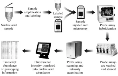
In the Affymetrix arrays each gene is represented as a probe set of 10 to 25 oligonu-cleotide pairs instead of one full length or partial cDNA clone. The oligonuoligonu-cleotide pair (probe pair) comprises of one oligonucleotide perfectly matching to the gene sequence (Perfect Match, PM) and a second oligonucleotide having one nucleotide mismatch in the middle of it (Mismatch, MM). Probes are designed within 500 base pairs of the 3’ end of each gene to hybridize uniquely in the same, predetermined hybridization conditions (Dalma-Weiszhausz et al.,2006;Brown et al.,1999;Tuimala & Laine,2003;Robinson & Speed,2007). See Figure1.1.

Figure 1.1 – Work flow of the Affymetrix microarray experiment.

Generally, the data is frommseries of experiments (samples) andngenes (gene expression matrix). Thus the gene expression matrix is represented as follows

G=       g11 g12 . . . g1m g21 g22 . . . g2m .. . ... . .. ... gn1 gn2 . . . gnm      

1.3 Literature Review

Recent literature has reported an increased spread of non-communicable dis-eases such as cancer (of all types). This has made cancer classification in early stages necessary to enhance disease diagnoses and prognoses. Such improvements in clas-sification will help physicians to choose the suitable treatment (Abusamra,2013) in

(25)

1.3. Literature Review

order to avoid negative outcomes such as death. The last decade has seen a grow-ing trend towards non-communicable disease classification usgrow-ing microarray gene expression data.

Over the past decades, biologists had to work hard to produce a small amount of data for use to explore a hypothesis with one observation at a time (Seidel,2008). When microarray gene expression was invented, one experiment can now generate thousands of observations. Hence, this has led to decrease in the amount of time needed to generate data.

Since the discovery of microarray technology, cancer classification research has rapidly gained attention. During the past few years contribution have been made in the literature regarding the classification of various type of cancers or cancer subtypes. Also, various classification methods have been applied to cancer. These methods include support vector machines (SVM), artificial neural networks (ANN), K-nearest neighbor (KNN), Naive Bayes (NB), and decision trees (DT). In addition ensemble methods such as Bootstrap aggregating (bagging) and Boosting are also among methods of interest.

Valentini(2002) applied the SVM with linear, polynomial, and radial basis ker-nel functions and multi-layer perceptrons (MLP) with one hidden layer on a lym-phoma, using gene expression data named Lymphochip (DNA microarray devel-oped at stanford university school of medicine). The data consisted of96tissue sam-ples from normal and malignant population of human lymphocytes, and4026 dif-ferent genes expressed in lymphoid cells with known roles in processes importance in immunology or cancer. The samples contained missing gene expression levels of about6%of all the data whose values were replaced with zeros. They considered two problems, which are the classification of cancerous and non cancerous lymphoid tissues, and the identification of Diffuse Large B-cell Lymphoma (DLBCL). The sec-ond problem above includes the Germinal Centre B-like DLBCL (GCB-like), and Activated B-like DLBCL (AB-like). The analysis showed that the SVM with a linear kernel had the best performance. For classifying malignant and normal tissues the author estimated the generalization error using 10 fold cross validation and found that SVM with linear kernel achieved the best results with1.04error and100% sensi-tivity. In identifying DLBCL subgroups, they performed5classification tasks using SVM and leave one out cross validation to estimate the generalization. For each clas-sification task performed using different expression signatures (proliferation, T cell, lymphnode, and genes that distinguish germinal centre B-cells from other stages in B-cell ontogeny (GCB expression signature)) and all signatures together, the results showed that SVM with RBF had good results on GCB expression signatures with 4%of an estimated generalization error and 91%sensitivity. That means GCB ex-pression signatures are specifically related to the separation of GCB-like and AB-like

(26)

subgroup of lymphoma inside the DLBCL group.

Wu et al.(2003) compared the performance of SVM, RF, KNN, LDA, quadratic discriminant analysis (QDA), and bagging and boosting classification trees, using an ovarian cancer mass spectrometry data. The dataset was obtained from the National Ovarian Cancer Early Detection Program at Northwestern University Hospital. This data set consists of MS spectra that extend from800to3500Da that were obtained on serum samples from 47 patients with ovarian cancer and 44 normal patients. Pre-processing were done using approaches such as taking the log of the intensities, background subtraction, and peak identification, etc. Thereafter, the feature selec-tion were done using two methods to select subset features. First they ranked the features based on thet-statistic, and used the RF to select the subset feature based on the a variable importance measure. Then they applied the classifiers on the data with 15and25selected markers (features) and compared their performance based on the prediction error rate using 10-fold cross validation and 0.632+ bootstrap methods. The results showed that the 0.632+ rule provides more stable estimates of the er-ror rate than 10 fold cross validation for some methods. Comparatively the results showed that RF and LDA performed well among other approaches. Using15 mark-ers selected using thet-statistic, SVM achieved the lowest error rate followed by the LDA method and the RF approach was among the top three. When the number of selected markers increases from15to25, SVM had the lowest error rate and RF fol-lowed closely in performance. While RF outperformed all the methods when the selected variable are derived from the importance measures based on RF. In gen-eral RF had lower prediction error rate than the minimum error rate obtained using variables selected throught-statistics.

Liu et al. (2005) proposed a novel analysis procedure, which involved reduc-ing the dimension usreduc-ing kernel principal component analysis (KPCA) and classi-fication using logistic regression (LR) for discrimination. Gene (features) selection was done based on the likelihood ratio, to obtain the most informative genes based on the highest likelihood ratio score. The proposed method was applied to five gene expression datasets involving human tumor samples such as leukemia, colon, lung cancer, lymphoma, and NCI. The procedure was then compared with SVM and ANN. Thereafter, the classification performance were assessed using the leave one out cross validation for all the datasets except for the leukemia data set which was based on one training and test data only. They showed that the new procedure was able to distinguish between different classes with high accuracy.

Delen et al.(2005) compared three methods, namely, ANN, decision trees (DT), and LR prediction models using a large dataset from breast cancer. The authors used data contained in the SEER cancer Incidence Public-Use Database for the years 1973 and 2000. This dataset contained of433,272records/cases and 72variables which

(27)

provided social demographic and cancer specific information. In an exploratory analysis of the data it was found40%of the records contained missing data. In the subsequent analysis the missing data were dealt with by removing the records with missing information leading to the so called complete case analysis. Furthermore, they examined the impact of removing these records on other variables and the anal-ysis showed there was no significant effect on the distribution of the variables. After the preliminary data cleaning and preparation for analysis step, the final analysis dataset consisted of16predictor variables with one dependent variable in a total of 202,932records. Their results indicated that the DT model was the best predictive model with93.6%accuracy on the holdout sample, while the ANN model had an accuracy of91.2%and the LR model an accuracy of89.2%.

Hu et al.(2006) conducted a comparison of five classification methods (LibSVMs, C4.5, BaggingC4.5, AdaBoostingC4.5, and RF) on seven distinct microarray cancer datasets, namely breast, lung, lymphoma, ALL-AML leukemia, colon, ovarian, and prostate. Preprocessing of the microarray data was done via information gain ratio for gene selection and used (Fayyad and Irani’s MDL) attribute discretization meth-ods. Ten fold cross validation was used for performance estimation. Two statistical methods, namely, the Wilcoxon signed rank test and sign test were used to vali-date the average accuracies of ten-fold cross validation on all the data sets. They showed that all the ensemble methods (BaggingC4.5, AdaBoostingC4.5, and RF) performed better than single-classification methods (LibSVMs, C4.5) and that the Wilcoxon signed rank test was better than the sign test.

In order to determine the best feature selection method,Haury et al.(2011) com-pared32 feature selections methods using five classification methods, namely, the nearest centroid (NC), KNN withk= 9, linear SVM withC= 1, linear discriminant analysis (LDA), and NB, to evaluate their performance. They showed that the simple t-test feature selection method provided the best results out of32feature selection methods among the classification methods used.

A more general comparative study on classification methods was performed byAbusamra(2013), who applied SVM, KNN, and RF, and eight different feature selection methods, namely, information gain, twoing rule, sum minority, max mi-nority, Gini’s index, sum of variances,t-statistics, and one-dimension SVM, on two publicly-available glioma datasets. Five-fold cross-validation was used to evaluate the classification performance. In terms of accuracy, the SVM approach was the best in comparison to all other models even before feature selection, due to its suitability for high dimensional data. These results suggest that by performing feature selec-tion, the accuracy of classification can be significantly improved by using a smaller number of genes.

(28)

1.4. Problem Statement

samples in which there were32acute lymphoblastic leukemia (ALL) samples and14 acute myleloid leukemia (AML) samples), using ANN but also compared the ANN approach to five other methods (SVM, NB, LR, KNN, and classification trees). This study applied the leave-one-out and ten-fold cross-validation methods to assess the performance of the methods using eight measures. ANN had a significant classi-fication accuracy of 98%on ten-fold cross-validation and leave-one-out approach. While, SVM had the second best classification accuracy of91%. Furthermore, ANN, KNN and NB simultaneously had the highest sensitivity. However ANN had both the highest sensitivity and specificity of100%and93%respectively.

Huang et al. (2018) concluded that SVM are a very powerful method in vari-ous fields, including cancer genomics, compared to the other methods. To date SVM have been applied in many application such as classification/ subtyping, biomarker/ signature discovery, drug discovery, driver gene discovery, and gene interaction. The success of SVM is partly related to the flexibility of any kernel approach and partly related to the robustness of SVM in the presence of bias in the training data.

A review of the literature suggests that SVM, KNN and RF are the three top most commonly used classification methods in microarray studies. In most of the previ-ous comparative studies, the methods have been evaluated based on a single cancer-type data (Abusamra,2013;Valentini,2002;Wu et al.,2003;Dwivedi,2016), without replication across the cancer spectrum, to ensure robustness. In studies that have employed different cancer-types, the comparisons have been between ensemble and single-classification methods (seeHu et al.(2006)). Generally, factors that influence performance of the classification methods such as microarray platform, disease un-der study and the gene selection method, have not been addressed (Novianti et al.,

2014). Consequently, none of the methods have been unanimously agreed upon as the best method in microarray based cancer classification.

In this study, we performed a comparative review of the SVM (with the linear, polynomial and radial basis kernels), KNN, RF, NB and ANN, in an attempt to iden-tify the best method for microarray-based cancer classification. The methods were evaluated based on classification accuracy, sensitivity, specificity, kappa coefficient, AUC, receiver operating curve (ROC), and BER (Stephens & Diesing,2014), using ten publicly-available microarray datasets from the same platform.

1.4 Problem Statement

Cancer tumor classification based on morphological characteristics alone has been shown to have serious limitations in some studies (Golub et al.,1999). The use of gene expression data from microarrays has improved the classification. However, numerous classification algorithms have been developed in this regard but none has

(29)

1.5. Objectives of the Study

been unanimously accepted as the best method for microarray data. Here, we seek to review these methods with the goal of identifying a superior method, based on publicly-available microarray data.

1.5 Objectives of the Study

The general objective of the thesis is to review cancer classification techniques, and apply these methods on publicly available microarray gene expression data. The specific objectives of this study are:

• To obtain and analyze microarray data from a public repository (GEO). • To perform gene selection, i.e. obtain a small panel of genes to employ as input

variables/predictors in the classification algorithms.

• To identify a classification method that can be regarded as the best method for cancer classification, based on certain statistical measures of performance.

1.6 The Structure of the Dissertation

This study is concerned with classification methods for disease applied to cancer datasets. There are five chapters in the dissertation, which are structured as follows: Chapter 1: This chapter introduces the study, by giving the background, a litera-ture survey, and the aims and objectives of the study.

Chapter 2: This chapter presents the background information on the data in gen-eral, a description of the each dataset used in the study, and a summary table for the datasets.

Chapter 3: In this chapter, we discuss the methods support vector machines, arti-ficial neural networks, naive Bayes, random forests, andk-nearest neighbor models as used in cancer classification. The write up explains the methodology and steps that will be used to compute the classification performance of each method.

Chapter 4: Here, we present results for each methods on the ten datasets. The results compares the performance of the different methods based on seven different measures of performance namely accuracy, sensitivity, specificity, kappa coefficient, ROC, area under the curve (AUC), and balanced error rate (BER).

Chapter 5: This chapter gives the discussion, conclusion and future research ar-eas emanating from the current research.

(30)

Chapter 2

Data description

In this study, we used ten gene expression datasets on the most common cancer-types among men and women, which were downloaded from Gene Expression Om-nibus (https://www.ncbi.nlm.nih.gov/geo/), with accession numbers

GSE23988, GSE7670, GSE8401, GSE10072, GSE10245, GSE25136, GSE35896,

GSE103091,GSE5851andGSE32962. The description for each dataset is as given below. Clinical information would have been useful. But not all datasets in GEO contain clinical information for the samples, which is a limitation in clinical studies. Table2.1below provides a concise summary of the gene expression datasets used in the study.

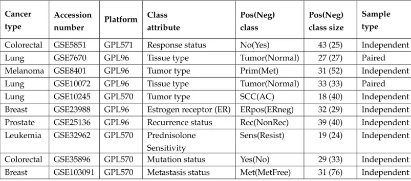
Table 2.1:Summary of the gene expression datasets used in the study. Here Pos and Neg represents positive and negative, respectivlely. GSE(GEO Sample), GPL(GEO Platform). Cancer type Accession number Platform Class attribute Pos(Neg) class Pos(Neg) class size Sample type

Colorectal GSE5851 GPL571 Response status No(Yes) 43 (25) Independent

Lung GSE7670 GPL96 Tissue type Tumor(Normal) 27 (27) Paired

Melanoma GSE8401 GPL96 Tumor type Prim(Met) 31 (52) Independent

Lung GSE10072 GPL96 Tissue type Tumor(Normal) 33 (33) Paired

Lung GSE10245 GPL570 Tumor type SCC(AC) 18 (40) Independent

Breast GSE23988 GPL96 Estrogen receptor (ER) ERpos(ERneg) 32 (29) Independent Prostate GSE25136 GPL96 Recurrence status Rec(NonRec) 39 (40) Independent Leukemia GSE32962 GPL570 Prednisolone

Sensitivity

Sens(Resist) 19 (24) Independent Colorectal GSE35896 GPL570 Mutation status Yes(No) 29 (33) Independent Breast GSE103091 GPL570 Metastasis status Met(MetFree) 31 (76) Independent

(31)

2.1. Dataset 1: GSE5851

2.1 Dataset 1: GSE5851

The dataset contains22,277probes from68metastatic colorectal cancer tumors, subjected to cetuximab monotherapy. Samples were classified by response status as either a non-responder (No) with43or a responder (Yes) with25cases ( Khambata-Ford et al., 2007). After filtration and normalization, 12,084genes were retained. Fourteen (14) differentially expressed genes between the two classes were employed in model training and validation downstream.

2.2 Dataset 2: GSE7670

The dataset consists of22,283probes from66lung adenocarcinoma tissues,27of which were matched normal-tumor samples (Su et al.,2007). Filtration and probe re-duction to one per gene resulted in12,084genes. Analysis of differentially expressed genes 19 paired training samples yielded 1,450genes for classification. Here, we used the tumor status (Tumor/Normal) as classification variable for model training and validation.

2.3 Dataset 3: GSE8401

The dataset consists of 22,283 probes from 83 samples. There are 31 primary (Prim) and52metastatic (Met) melanoma tumors from patients undergoing surgery, collected from 1992 to 2001 as a part of the diagnostic work-up or therapeutic strat-egy (Xu et al.,2008). Probe filtration and reduction to one per gene yielded12,084 genes, of which1,483were differentially expressed between the59training primary and metastatic samples. Model training and validation were based on1,483genes.

2.4 Dataset 4: GSE10072

There was a total of22,283probes from each of the33paired (tumor and normal) samples used in this analysis (Landi et al.,2008). Filtration reduced the initial22,283 probes to 12,084 genes, of which 3002 were differentially expressed genes hence were selected for model training and validation.

2.5 Dataset 5: GSE10245

The dataset contains54,675probes from58non-small cell lung cancer (NSCLC) tumor samples, classified as either adenocarcinoma (AC) with40or squamous cell carcinoma (SCC) with18cases (Kuner et al.,2009). Filtration reduced the probes to

(32)

2.6. Dataset 6: GSE23988

18,978genes, and differential expression analysis selected819genes from41training samples, for model training and validation.

2.6 Dataset 6: GSE23988

The dataset consists of22,283probes taken from61patients with HER2-normal stage I-III breast cancer who received preoperative chemotherapy to identify gene sets associated with pathological complete response to therapy (Iwamoto et al.,2010). Estrogen receptor (ER) status (32 ERpos) and (29 ERneg) was used as the class at-tribute. After filtration and normalization,12,084genes were retained, out of which 579were selected for model building and validation.

2.7 Dataset 7: GSE25136

The dataset consists of22,283probes from79prostate cancer tumors, classified as either having disease recurrence (Rec) with39or non-recurence (NonRec) with40 cases. Recurrent status was used as the positive class in the model building and val-idation processes (Sun & Goodison, 2009). Filtration reduced the probes to12,084 genes, and differential expression analysis selected52 genes from56 training sam-ples, for model training and validation.

2.8 Dataset 8: GSE32962

The dataset contains 54,517 probes from blood samples from 43 infants with Acute Lymphoblastic Leukemia (ALL), subjected to prednisolone treatment. The samples were classified by prednisolone sensitivity as either sensitive (Sens) with19 or resistant (Resist) with24cases (Spijkers-Hagelstein et al.,2012). Filtration reduced the probes to 18,956genes, of which 117genes were differentially expressed and used for model training and validation.

2.9 Dataset 9: GSE35896

The dataset contains54,675probes from62 colorectal cancer tumors, classified by KRAS mutation status as either a KRAS-mutant (Yes) with29or KRAS wild-type (No) with33cases sub-type (Schlicker et al.,2012). Filtration reduced the probes to 18,978genes. Differential gene expression analysis yielded43 genes, based on 45 training samples, for subsequent model training and validation.

(33)

2.10. Dataset 10: GSE103091

2.10 Dataset 10: GSE103091

The dataset also contains54,675probes from107primary breast tumours (J´ez´equel et al., 2015). The tumors were classified by metastasis status as either metastatic (Met) with31or metastatis-free (MetFree) with76cases, with metastasis-free as the positive class attribute. Probe filtration and reduction to one per gene yielded18,978 genes. Differential gene expression analysis resulted in a54gene list, which was em-ployed in model training and validation.

(34)

Chapter 3

Methodology

Several methods have been developed for classification using microarray gene expression data, each with its advantages and disadvantages. In this study, we present a comparative analysis of seven classification methods using ten cancer datasets described in Chapter 2. Below we present an overview of each method.

3.1 Support Vector Machines (SVM)

The SVM method was first presented byBoser et al.(1992) at the Computational Learning Theory (COLT92) ACM Conference in 1992. SVM are based on the idea of the plane that lies furthermost from both classes. This plane is known as theoptimal (maximum) margin hyperplane. The hyperplane is completely determined by a sub-set of the samples known as thesupport vectors(Moguerza & Mu ˜noz, 2006). SVM have the ability to handle problems where the data are not linearly separable by transforming the data using mapping kernel functions such as the radial basis func-tion (RBF) kernel, polynomial funcfunc-tion, and the linear funcfunc-tion (Stephens & Diesing,

2014). Moreover, SVM have strong capability in handling high dimensional data, which is clearly an add advantage. Accordingly, this strength makes SVM widely ap-pealing and have been successfully applied to real-life data analysis problems such as handwritten character recognition, human face recognition, radar target identifi-cation, speech identifiidentifi-cation, and gene expression data analysis (Brown et al.,1999;

Chu & Wang,2003).

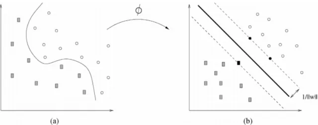
Suppose we have msamples and ngenes. Further, assume samples belong to two distinct outcome classes represented by+1or −1and a feature vectorg_i such that (g_i, yi) ∈ G×Y i = 1,2, . . . m, whereg_i = (gi1, gi2, . . . , gin)0 is the sample profile (vector) and yi ∈ {+1,−1} is the outcome class dichotomy. The goal is to classify the samples into the two classes by training the SVM to map the input data (using a suitable kernel function) onto a high-dimensional space (feature space)

(35)

3.1. Support Vector Machines (SVM)

(Φ(g_i), yi) m

i=1. This is achieved by constructing an optimal separating hyperplane that lies furthest from both classes (see Fig3.1).

The general form of a separating hyperplane in the space of the mapped data is defined by

wTΦ(g) +b= 0. (3.1)

Here,w= (w1, w2, . . . , wn)0, is the weight vector. We can rescale thewandbsuch that the following equation determines the point in each class that is nearest to the hyperplane

|wTΦ(g) +b|= 1. (3.2) Therefore, it should follow that for each samplei,i∈ {1,2, . . . , m},

wTΦ(g_i) +b=    ≥1 if yi = +1 ≤ −1 if yi=−1 (3.3)

After the rescaling, the distance from the nearest point in each class to the hy-perplane is _k_w1_k. Thus, the distance between the two classes is _k_w2_k, which is called themargin. To maximize the margin, the following optimization problem has to be solved min w,b kwk 2 _(3.4) subject to yi(wTΦ(g_i) +b)≥1, i= 1,2, . . . , m. (3.5) The square in the norm ofwis introduced to make the problem quadratic. Sup-posew∗ andb∗ are the solutions to Eq (3.4). Then this solution determines the hy-perplane in the feature space where (w∗)TΦ(g) +b∗ = 0. The points Φ(g_i) that satisfy the qualitiesyi((w∗)TΦ(g_i) +b∗) = 1 are calledsupport vectors as shown in Fig3.1(b) (Moguerza & Mu ˜noz,2006). There are many packages inRfor SVM im-plementation (e.g. e1071 package), but we have chosen thekernlabpackage because it contains various kernelized learning algorithms and all the features that we need as well, Moreover,kernlabis customized for kernel methods inR(Karatzoglou et al.,

(36)

3.1. Support Vector Machines (SVM)

Figure 3.1 – (a) Original data in the input space. (b) Mapped data in the feature space.

3.1.1 Kernel Function

The real world problems are not usually linearly separable. Therefore, there is need for a function which maps the original space to some higher dimensional fea-ture space where the training set is separable. Thus, we need to find a non-linear transformation functionΦ(g), to achieve this task hence a class of functions called kernels is used.

A kernelK(g,y) is a real valued functionK : GXG → _Rfor which there exist a functionΦ : G→ Z, whereZ is a real vector space, with the propertyK(g,y) = Φ(g)TΦ(y).

The kernelK(g,y)acts as a dot product in the space ofZ. In the literatureGand

Zare called input space and feature space, respectively. As well as, theK(g,y)must satisfy Mercer’s condition, hence it is known as a Mercers kernel.

There are many kernel functions, and in Table 3.1 below we present the ones used in the current study.

Table 3.1:Kernel Functions.

Name Kernel Function

Linear K(g,y) =gT_y

P olynomial K(g,y) = (c+gTy)d

RadialBasisF unction(RBF) K(g,y) = exp(−γ||g−y||2₎

Wherecis the constant value,dis the polynomial degree, andγis a parameter that sets the spread of the kernel, it defines how far the influence of a single training example reaches. Intuitively, a small gamma value define a Gaussian function with a large variance.

(37)

3.2. Artificial Neural Networks (ANN)

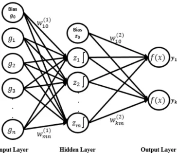
3.2 Artificial Neural Networks (ANN)

Artificial neural networks (ANN) are multi-layered models that are constructed from three layers, each layer consisting of nodes calledneurons(Dwivedi,2016). The input layer contains nodes whose number is based on the input features. The output layer contains nodes equal to the number of classes, and finally the hidden layer con-tains nodes determined by the level of tuning required. The inputs are weighted by multiplying each input by a weight as a measure of its contribution. The layers are connected together via connection weights. These weights are determined through stages of model fitting. The hidden nodes receive the sum weighted from the input layer plus some bias. This summation is passed onto the transform function (activa-tion func(activa-tion) to generate the results. These results are calledoutputsand interpreted as class probability in our case.

There are many types of architectures of ANN. The choice of the number of hid-den layers is an important part of deciding the overall neural network architecture and can affect the results. Here, we used the default setting for thennet package, which is the single hidden layer and is sufficient for our purposes. Neural networks are used widely in different fields such as prediction in time series models, economic modeling and medical applications among others (Stephens & Diesing, 2014). In addition, ANN can be applied to the classification problem using microarray gene expression data (Dwivedi,2016).

Consider the simplest multi-layered network, with one hidden layer, as in Fig3.2 below. Assume we have gene expression data wherendenotes the number of genes. Then the input layer receives thengene expression levels for a sample, each multi-plied by the corresponding weight,w_ij(1)gj, as shown in Eq3.6, below:

bi = n

X

j=0

w_ij(1)gj i= 1,2, . . . , m, (3.6)

whereg = (g0, g1, g2, . . . , gn)0 is a vector of input features andg0 = 1is a constant input feature with weightwi0. The quantities, bi, are calledactivations, and the pa-rametersw_ij(1)are the weights. Note that alternativelybican be viewed as a summary of thengenes from samplei. The superscript“(1)”indicates that this is the first layer of the network. Each of the activations is then transformed by a nonlinear activation functionf, typically a sigmoid, as in Eq3.7below:

zi =f(bi) =

1 1 + exp(−bi)

(38)

3.2. Artificial Neural Networks (ANN)

The quantitiesziare interpreted as the output of hidden units, so called because they do not have values specified by the problem (as is the case for input units) or target values used in the training (as is the case for output units).

In the second layer, the outputs of the hidden units are linearly combined to give the activations of theKoutput units:

ak= m

X

i=0

w(2)_ik zi k= 1,2, . . . , K. (3.8) Again,z0 = 1corresponds to the bias. The transformations in the second layer of the neural networks are parameterized by weightsw(2)_ik . The output units are transformed using an activation function. Again, a sigmoid function may be used as shown below:

yk =f(ak) =

1 1 + exp(−ak)

. (3.9)

These equations may be combined to give the overall equation that describes the forward propagation through the network, and describes how an output vector is computed from an input vector, given the weight matrices as

yk =f   m X i=0 w(2)_ik  f   n X j=0 w_ij(1)gi      . (3.10)

ANN are implemented using theRpackagennet, because it is the simplest one and restricted to a single layer (Ripley et al.,2016).

(39)

3.3. Naive Bayes (NB)

Figure 3.2 –Multi-layer neural networks architecture.

3.3 Naive Bayes (NB)

The Naive Bayes classifier uses probability theory to find the most likely of the possible classes in a classification problem. The NB classifier relies on two assump-tions, namely, that each attribute is conditionally independent from the other at-tributes given the class and that all the atat-tributes have influence on the class (De Cam-pos et al., 2011). The popularity of this classifier is mainly due to its simplicity, yet exhibiting a surprisingly competitive predictive accuracy. The NB classifier has previously been applied in many fields, including microarray gene expression data (Stephens & Diesing,2014;Dwivedi,2016).

Consider anmbyngene expression data matrix, wheremis the number of the samples andnis the number of the genes (features). Letgkj, j = 1,2, . . . , n, denote thej-th gene on thek-th sample. LetCibe thei-th class,i= 1,2, . . . , L. The Naive Bayes classifier uses the maximum a posteriori (MAP) classification rule to classify these samples. The probability of thek-th sample vector,Gk = (gk1, gk2, . . . , gkn)0, is calculated and then the sample is assigned the class with largest probability from

Lconditional probabilities. That is, let P(C1|Gk), P(C2|Gk), . . . , P(CL|Gk) denote the set ofLconditional probabilities. The NB classification depends on the Bayes rule, which states that a posterior probability

P(Ci|Gk) =

P(Gk|Ci)P(Ci)

P(Gk)

(40)

3.4. Random Forests (RF)

whereP(Gk)is considered a common factor for all theLprobabilities.

The NB classification assumes all input features are conditionally independent, that is,

P(gk1, gk2, . . . , gkn|Ci) =P(gk1|gk2, . . . , gkn, Ci)P(gk2, . . . , gkn|Ci)

=P(gk1|Ci)P(gk2, . . . , gkn|Ci)

=P(gk1|Ci)P(gk2|Ci). . . P(gkn|Ci)

(3.12)

Ultimately, NB classifies a new sample, G∗, according to the model with MAP probability given the sample, as

Class(G∗)M AP =argmax(P(Ci|G∗)). (3.13) NB are implemented using theRpackagenaivebayes.

3.4 Random Forests (RF)

Random forests were first introduced in 2001 (Friedman et al., 2001; Breiman,

2001). They are an extension of classification and regression trees, and also an im-provement over bagged trees by the way of a random small tweak to de-correlate the trees. Growing random forests leads to an improvement in prediction accuracy com-pared to single or bagged trees (Qi,2012). We build a number of forests of decision trees on bootstrapped training samples from the original data. A tree is obtained by recursively splitting the genes set of sizep. At each node of the tree, a candidate gene for splitting is obtained from a random sample of sizev. A typical choice forv

is such thatv ≈√p. We then grow the trees to maximum depth. Therefore, the two step randomization help to decorrelate the trees (Chen & Ishwaran,2012). To deter-mine the prediction for an unknown sample, an average over all the trees is taken for a regression problem and a majority vote for a classification problem (Friedman et al.,2001;Pappu & Pardalos,2014;Do et al.,2009).

Random Forests Algorithm for Regression or Classification (Friedman et al.,2001)

1. Forb= 1toB(#random-forest trees):

• Draw a bootstrap sample of sizeN from the training data.

• Grow a random-forest tree, Tb to the bootstrapped data, by recursively repeating the following steps for each terminal node of the tree, until the minimum node size,nmin, is reached.

(41)

3.5. k-Nearest Neighbor (KNN)

(b) Pick the best gene to split on among thevbased on an impurity mea-sure.

(c) Using the selected gene, split the node into two daughter nodes. 2. To make a prediction for a new sample,x:

LetCˆb(x)be the class prediction of theb-th random-forest tree. Then

ˆ

C_rfB(x) =majority votenCˆb(x)

oB

b=1

Random forests comprise a number of decision trees, and each node in the decision tree is a condition on a single feature, which divides the data into two. Ginis index was used for the impurity measure in this work because it is the best for classification problems (Pal,2005;Breiman et al.,2011). Ginis index is a measure of how often a randomly chosen element from a set would be incorrectly labeled if it was randomly labeled according to the distribution of labels in the subset. It is computed as

Gini(D)= 1− m

X

i=1

p2_i

WhereDis a set of training samples and their associated class labels belongs to class

i,piis the probability that a sample inD, the sum is computed overmclasses. RF are implemented using theRpackagerandomForest(Breiman et al.,2011).

3.5 k-Nearest Neighbor (KNN)

Thek-nearest neighbor classifiers (KNN) are known to be most useful instance-based learners. KNN is a non-parametric model (Yao & Ruzzo,2006). If the classifi-cation is based on Euclidean distance in feature space, thenkdetermines the number of neighbors to be used. In the testing set assign the new sample the class that is most likely among thekneighbors. The number of neighbors can be tuned to choose the optimal value ofk(Stephens & Diesing,2014;Dwivedi,2016).

There are many types of similarity measure, such as Euclidean distance, cosine similarity, and Mahalanobis distance. Theknnfunction uses the Euclidean distance as the default to find thek-th neighbors. Moreover, the Euclidean distance is sim-ple and works well with continuous data (Wilson & Martinez,1997;Ding & Peng,

2005). Since the gene expression data is continuous, the Euclidean distance was the preferred similarity measure.

The KNN uses the Euclidean distance measure to find the closest samples for the new sample. Suppose we have two samples, each one containingngenes. Specifi-cally denote the two samples asS1 = (g11, g12, . . . , g1n)0andS2 = (g21, g22, . . . , g2n)0.

(42)

3.6. Performance Measures

Then the Euclidean distance is calculated as squared root of the sum of the squared differences in their corresponding values. Using the Euclidean distance definition, the distance between two points, dist(S1, S2), is given as

dist(S1, S2) = v u u t n X j=1 (g1j−g2j)2. (3.14) Figure3.3below present the idea of thek-nearest neighbor.

Figure 3.3 –k-nearest neighbor approach.

3.6 Performance Measures

In this paper, the comparison was based on seven performance measures, as de-fined below. These measures were calculated from the generic confusion matrix below.

Table 3.2:Structure of the confusion matrix True Condition

Predicted Condition Positive Negative Positive True Positive (TP) False Positive (FP) Negative False Negative (FN) True Negative (TN)

1. Accuracyis the percentage of correctly classified samples:

Accuracy= T P +T N

A comparison of cancer classification methods based on microarray data.

A Comparison of Cancer

Classification Methods Based

on Microarray Data

A Comparison of Cancer Classification Methods

Based on Microarray Data

Declaration - Plagiarism

Disclaimer

Abstract

Dedication

Acknowledgements

Contents

List of Figures

List of Tables

Abbreviations

Chapter 1

Introduction

1.1

Background

1.2

Microarray Technology

1.3

Literature Review

1.4

Problem Statement

1.5

Objectives of the Study

1.6

The Structure of the Dissertation

Chapter 2

Data description

2.1

Dataset 1: GSE5851

2.2

Dataset 2: GSE7670

2.3

Dataset 3: GSE8401

2.4

Dataset 4: GSE10072

2.5

Dataset 5: GSE10245

2.6

Dataset 6: GSE23988

2.7

Dataset 7: GSE25136

2.8

Dataset 8: GSE32962

2.9

Dataset 9: GSE35896

2.10

Dataset 10: GSE103091

Chapter 3

Methodology

3.1

Support Vector Machines (SVM)

3.2

Artificial Neural Networks (ANN)

3.3

Naive Bayes (NB)

3.4

Random Forests (RF)

3.5

k-Nearest Neighbor (KNN)

3.6

Performance Measures