Systemic Risk from Global Financial
Derivatives: A Network Analysis of Contagion
and Its Mitigation with Super-Spreader Tax
© 2012 International Monetary Fund WP/
Monetary and Capital Markets Department
Systemic Risk from Global Financial Derivatives: A Network Analysis of Contagion and Its Mitigation with Super-Spreader Tax
Prepared by Sheri M. Markose1
Authorized for distribution by Aditya Narain
Abstract
JEL Classification Numbers: JEL: G01, G21, G17, G32, G15
Keywords: Systemic Risk; Financial Network; Too-Interconnected-to-Fail; Eigenvector Centrality; Super Spreader Tax.
1 Sheri Markose, ([email protected]) is a professor in the Economics Department at the University of Essex,
United Kingdom and was a consultant to the IMF when this paper was written. This draft of the paper reflects the reviews from Emanuel Kopp, Manmohan Singh, Mohammed Norat and André Santos. I would like to thank participants for their comments at the presentation of the paper at the IMF on December 7, 2011, the Financial Stability Group of the Bank of England on February 13, 2012 and the Kiel Institute for the World Economy Summer School on 26-27 June 2012. I also thank the following for their helpful inputs: Aditya Narain, David Bholat, Thomas Lux, Daniel Fricke, Jorge Chan-Lau, Karl Habermeier, Laura Kodres, Jodi Scarlata and Anna Ilyina. Research assistance from Edna Solomon was vital in the collection of data. The software for computational and visual outputs in this project was jointly developed by me with Simone Giansante and Ali Rais Shaghaghi. All errors and omissions are my sole responsibility.
This Working Paper should not be reported as representing the views of the IMF.
The views expressed in this Working Paper are those of the author(s) and do not necessarily represent those of the IMF or IMF policy. Working Papers describe research in progress by the author(s) and are published to elicit comments and to further debate.
Financial network analysis is used to provide firm level bottom-up holistic visualizations of interconnections of financial obligations in global OTC derivatives markets. This helps to identify
Systemically Important Financial Intermediaries (SIFIs), analyse the nature of contagion propagation, and also monitor and design ways of increasing robustness in the network. Based on 2009 FDIC and
individually collected firm level data covering gross notional, gross positive (negative) fair value and the netted derivatives assets and liabilities for 202 financial firms which includes 20 SIFIs, the bilateral flows are empirically calibrated to reflect data-based constraints. This produces a tiered network with a distinct highly clustered central core of 12 SIFIs that account for 78 percent of all bilateral exposures and a large number of financial intermediaries (FIs) on the periphery. The topology of the network results in the “Too- Interconnected-To-Fail” (TITF) phenomenon in that the failure of any member of the central tier will bring down other members with the contagion coming to an abrupt end when the ‘super-spreaders’ have demised. As these SIFIs account for the bulk of capital in the system, ipso facto no bank among the top tier can be allowed to fail, highlighting the untenable implicit socialized guarantees needed for these markets to operate at their current levels. Systemic risk costs ofhighly connected SIFIs nodes are not priced into their holding of capital or collateral. An eigenvector centrality based ‘super-spreader’ tax has been designed and tested for its capacity to reduce the potential socialized losses from failure of SIFIs.
Contents Page
Abstract ...1
I. Introduction ...4
II. Systemic Risk in OTC Derivatives: Modeling Challenges ...8
A. SIFIs in Derivatives Markets and Market Concentration ...8
B. Market Data Based Systemic Risk Measures and Financial Network Perspective .12 III. Financial Network Analysis ...16
A. Adjacency Matrix and Gross Flow Matrix for Derivatives ...16
B. Bilaterally Netted Matrix of Payables and Receivables ...17
C. Topology of Financial Networks Complete, Random, Core-periphery, Clustered, and Small World ...18
D. Economics Literature on Financial Networks ...23
E. Eigenvalue Perspective of Network Stability ...25
IV. Contagion and Stability Analysis ...26
A. Furfine (2003) Methodology: Cascades from Failure of a Trigger Bank ...27
B. Financial Network Stability Analysis ...28
C. Mitigation and Management of Financial Contagion: Super-spreader Tax ...33
V. Empirical Results: Network Analysis of the Calibrated Aggregated Global Derivatives Market ...35
A. Empirical (Small World) Core-Periphery Network Algorithm ...36
B. Global Derivatives Network Statistics (2009:Q4) ...38
C. Eigenvector Centrality and Furfine Stress Test Results ...40
D. Quantification and Evaluation of the Super-spreader Tax (2009 Q4) ...44
VI. Conclusion ...47
References ...52
Tables 1. Value and Market Share of Financial Derivatives for 202 FIs ...11
2. Networks Statistics: Diagonal Elements Characterize Small World ...20
3. Network Statistics for Degree Distribution for Derivatives Network 2009 Q4 ...39
4. Rich Club Statistics ...40
5. 2009:Q4 Derivatives Network Eigenvector Centrality and Furfine First Round Contagion Results for Top 20 FIs ...41
6. Super-Spreader Tax Raised from Top 20 SIFIs ...47
Figures 1. Gross Notional of Financial Derivatives...5
2. Gross Market Values OTC Derivatives ...6
3. Affiliation Graph of Global SIFIs and United States (U.S.) FDIC FIs as Participants in the Five Financial Derivatives Markets ...10
4. Empirically Constructed Global Derivatives Network (Bilaterally) Aggregated over all Derivatives Products for FIs and Outside Entities: Empirical Small World Network in Tiered Layout ...37 5. Furfine Contagion Stress test on Empirical Calibrated Derivatives ...43 6. Maximum Eigenvalue (#
max ,Y-Axis) Using Different Values of > 0(Equation ...45 7. Individual FI Tax Rates Obtained by Multiplying Right Eigenvector Centrality by or Different Values of Alpha >0 ...46
Appendix Tables
I. INTRODUCTION
Systemic risk from financial derivatives markets came to the forefront with the accelerated growth in credit derivatives to about US$60 trillion at its peak in 2007.
Excessive liabilities from a small segment of credit default swaps (CDS) on residential mortgage-backed securities for key institutions such as American Insurance Group (AIG) threatened to destabilize the financial system. The collapse of the United States (U.S.) house prices triggered widespread weakness in this class of credit derivatives that had initially helped in the proliferation of U.S. mortgage backed securities globally, leading to the unprecedented taxpayer bailouts of financial institutions estimated at over US$14 trillion over the course of the 2007̶8 financial crisis (Alessandri and Haldane (2009)). The bailouts premised a moral hazard problem identified asarising from some financial institutions being “Too- Interconnected-To-Fail” (TITF), with threats to the financial system as a whole following from domino effects of the failed entity on others. The AIG bailout aimed to stem the negative externalities of its failure to deliver on its CDS guarantees to major
counterparties.2 The correlated jump to default spikes in CDS premia for contracts for which
Lehman Brothers was the protection seller and the triggering of CDS on Lehman Brothers as the reference entity is estimated to have magnified liquidity demands during the conditions, which led to a ‘run’ on the wholesale money markets in 2008 (Gorton and Metrich (2009)).3 The objective of this paper is to quantitatively model the contagion-like threats posed by the activities of large financial intermediaries in the over-the-counter (OTC) derivatives markets using network analysis. The size of gross notional amounts
outstanding of OTC derivatives globally is estimated by Bank for International Settlements (BIS) Statistics at over US$614 trillion in December 2009.4 Of this, in 2009:Q4 the gross
2 Of the US$170 billion U.S. tax payer bailout of the American International Group (AIG), the initial
US$85 billion payment to AIG was geared toward honoring its CDS obligations totaling over US$66.2 billion. These include payouts to Goldman Sachs (US$12.9 billion), Merrill Lynch (US$6.8 billion), Bank of America (US$5.2 billion), Citigroup (US$2.3 billion), and Wachovia (US$1.5 billion). Foreign banks were also beneficiaries, including Société Générale and Deutsche Bank, which each received nearly US$12 billion; Barclays (US$8.5 billion), and UBS (US$5 billion). (Source: March 15, 2009 press release “AIG Discloses Counterparties to CDS, GIA, and Securities Lending Transactions”). Likewise, the Standard and Poor Report of August 2008, attributes the take-over of Merrill Lynch by Bank of America in 2008 to the failure of a little known Monoline called ACA Financial Guaranty Corporation (ACA) to deliver CDS cover for US$5 billion of Merrill’s balance sheet mortgage backed securities, which had a total of US$18.8 billion of CDS guarantees.
3 The gross notional value of the CDS obligations of Lehman Brothers, ranked the 10th largest counterparty, is
placed at between US$5trillion and US$3.65trillion (Financial Times, September 15 2008). The novation losses of CDS contracts for which Lehman was a counterparty are given at between UK£30 billion–US$50 billion. Of the US$400 billion, CDS with Lehman Brothers itself as the reference entity on a face value of its bonds of US$158 billion had recovery rate of as little as 8.625 cents per dollar, the net CDS settlement on this was about US$6 billion. Given the very small percentage of CDS positions being hedges on Lehman bonds (Das, 2010), the direct losses on Lehman bonds were close to US$150 billion.
notional of derivatives traded by deposit-insured U.S. financial institutions is
US$212.8 trillion and closer to US$285 trillion when commercial banks and others are included as holding companies.5 The exchange traded derivatives, in contrast, are valued at
no more than about US$73.14 trillion for 2009:Q4 and these are mostly futures and options contracts.6 When compared to the size of world GDP at US$70 trillion and the size of the
global bond market (total debt outstanding) at about US$82 trillion, the implication is that the size of off-balance sheet activities of financial intermediaries (FIs) has grown to many
multiples of their assets. Derivatives obligations of FIs under conditions of market-wide adverse movements on the underlying (such as interest rates, house prices, exchange rates, corporate debt and equity, and sovereign debt) could overwhelm the equity and assets of FIs.
Figure 1. Gross Notional of Financial Derivatives (in billions of dollars)
Source: BIS, June 2010 Quarterly Review.
5 The Q4 2009 OCC Quarterly Report, in Table 3, also gives the split between exchange traded and OTC
derivatives activity for U.S. FDIC commercial banks and Trust companies, respectively, as 3.9 percent (US$8.23 trillion) and 96.1 percent (US$204.58 trillion). However, when the estimates are done for the top 25 U.S. Bank Holding Companies (Table 2 of Consolidated Financial Statements for Bank Holding Companies, FRY-9 Schedule HC-L) there is considerable increase in derivatives activities for Morgan Stanley
(US$41.505 trillion with US$1.822 trillion in exchange traded), Bank of America (US$28.213 trillion with US$2.26 trillion of this exchange traded) and non FDIC entities of Taunas Corporation, Barclays Group U.S., GMAC and MetLife totaling US$1.91 trillion of which US$478.348 million is exchange traded).
6 See,Table 23A BIS Quarterly Review Statistical Annex, June 2010. Centrally cleared credit derivatives (not to
be confused with exchange traded derivatives which furnish pre trade price transparency) which include indices, sovereigns, and single name corporate reference entities are mostly being cleared by ICE Clear Credit in the U.S. and ICE Clear in Europe. Since their respective launches in March 2009 and July 2009, to date, a total of US$23.73 trillion gross notional CDS has been centrally cleared. For June end 2010, the BIS Quarterly Review (December 2010) shows that the CCP is the counterparty to US$3.3 trillion gross notional CDS contracts.
0 100000 200000 300000 400000 500000 600000 700000 800000 0 10000 20000 30000 40000 50000 60000 70000 Jun. 1998 Dec. 1998 Jun. 1999 Dec. 1999 Jun. 2000 Dec. 2000 Jun. 2001 Dec. 2001 Jun. 2002 Dec. 2002 Jun. 2003 Dec. 2003 Jun. 2004 Dec. 2004 Jun. 2005 Dec. 2005 Jun. 2006 Dec. 2006 Jun. 2007 Dec. 2007 Jun. 2008 Dec. 2008 Jun. 2009 Dec. 2009 Jun. 2010
Foreign exchange contracts Equity-linked contracts Commodity contracts Credit default swaps
Figure 2. Gross Market Values OTC Derivatives (in billions of dollars)
Source: BIS, June 2010 Quarterly Review.
Figures 1 and 2 give the gross notional and the gross market value of the global derivatives in the 5 different derivatives products. Since 2008, there has been a
considerable decline in both gross notional and gross market value due to compression and tear ups of bilateral positions. Gross notional is the best measure of the size of derivatives activity and the gross market value gives an estimate of the economic risk in derivatives arising from the volatility of underlying reference/asset prices, leverage and hedge ratios, duration, liquidity, and counterparty risk. Toward, the latter part of 2010, the increase in gross market value of derivatives can be attributed to growing volatility in financial markets.
At least since the NBER paper by Darby (1994), risk from financial derivatives has been considered a systemic threat due to the sheer size of the OTC markets and the high concentration of financial obligations. To this may be added the institutional weakness of OTC derivatives market (Duffie, (2010)) and correlated movements
(Brunnermeier et. al., (2009)) in the underlying assets of financial derivatives, interest rates, exchanges rates, bank assets, corporate and sovereign debt that can exacerbate the size of derivatives liabilities and also trigger multiple obligations across many sectors. In view of the growing structural concentration in the provision of risk guarantees through financial
derivatives, as will be reviewed next, the fragility of the modern risk sharing institutions are germane to issues on systemic risk. Existing statistical models for systemic risk may fail to identify the threats to stability from the topological structures of financial networks often referred to as TITF arising from the concentration of financial links between a few key players. The use of network analysis can help to identify systemically important players in terms of network connectivity, to assess the nature of contagion propagation, and also to monitor and design ways of increasing robustness of the network.
0 5000 10000 15000 20000 25000 30000 35000 40000 0 1000 2000 3000 4000 5000 6000
Foreign exchange contracts Equity-linked contracts Commodity contracts Credit default swaps Total contracts(right axis)
Systemic risk implications of a FI’s connectivity and concentration of obligations, by virtue of being a negative externality, have not been factored into the capital or collateral being held by FIs. Many have remonstrated (Acharya and Richardson (2009), Bernanke (2009)) against the socialization of losses from large complex FIs and have pointed out the need for highly connected FIs to internalize their systemic risk costs. In a ratings based system, as succinctly pointed out by Haldane (2009), leniency of capital and collateral requirements for a few large highly rated financial intermediaries has resulted in excessive expansion of credit and derivatives activities by them that is far beyond what can be
sustained in terms of system stability. Further, the expectation that FIs that are TITF will be bailed out also increases their ratings than if this were not to be the case (Moodys (2011), Haldane (2010)). Haldane (2009) calls such highly interconnected FIs ‘super-spreaders’ and this epithet will be retained in the financial network modeling that follows. Haldane (2009) recommends that super-spreaders should have larger buffers. To date, the financial networks literature have produced interesting qualitative analysis for contagion in networks, but have not operationalized a metric for systemic risk for the network system nor a measure of a FI’s contribution to systemic risk arising from the interconnectivity of its financial obligations. This paper is novel in proposing a systemic risk measure directly related to the stability of the financial network topology and a corresponding eigenvector centrality based ‘super-spreader’ tax to reduce the potential socialized losses from failure of highly interconnected FIs in the derivatives markets.
Section II will review the data on the derivatives markets to assess the modeling challenges posed by SIFIs (Systemically Important Financial Institutions) that dominate these markets. As the topological fragility arising from TIFT looms large, the extant market data-based methods for estimating systemic risk from FIs will be contrasted with the so called eigen-pair method for financial network stability analysis proposed in this paper. The market data-based methods for systemic risk modeling are found to run into the so called paradox of instability (Borio and Drehmann (2009), Minsky (1982)) that underscores the need to focus on a network model of direct financial exposures and obligations. Section III will review the technical aspects of network theory and economics literature on financial networks. The main drawbacks of the pre-2007 economics literature on financial networks have been that models that are based on empirical bilateral data between counterparties were few in number to establish ‘stylized’ facts on network structures for the different classes of financial products ranging from contingent claims and derivatives, credit related interbank exposures, and large value payment and settlement systems. Where bilateral data on financial exposures were not available, both empirical and theoretical models assumed network
structures to be either uncorrelated and random as in Nier et. al.(2007) or complete networks as in Upper and Worms (2004). As will be argued, these approaches crucially do not have the TITFcharacteristics that will be modelled using a highly sparse core-periphery network structure. Only Craig and von Peter (2010) and Fricke and Lux (2012) who use empirical bilateral interbank data have highlighted the core-periphery network structure that has also been found by the author to be most pronounced in the bilateral data for derivatives liabilities
in the Indian financial system.7 While the stability of financial networks has been usually investigated using the classic Furfine (2003) algorithm, sufficient emphasis has not been given to the way in which contagion propagates in highly tiered and clustered networks and stability of the system in terms of network characteristics has not been studied by
economists. Following May (1972, 1974) and the recent approach of Wang et. al. (2003) and Giakkoupis et. al.(2005), which is increasingly being adopted in epidemiology and for internet security, the maximum eigenvalue for the network of derivatives liabilities expressed as a ratio of Tier 1 capital will be used to determine the stability of the system.
Section IV discusses the necessary network stability results using maximum eigenvalue and the corresponding eigenvector centrality of the FIs. Systemic risk index for each FI is based on its right eigenvector centrality and the super-spreader tax fund that can mitigate potential socialized losses from the failure of highly connected banks is designed. In contrast, the left eigenvector centrality index for the financial network will be called the vulnerability or exposure index. In the empirical Section V, the empirical reconstruction of the derivatives network based on 2009:Q4 data is undertaken and the network analysis and a series of stress tests are conducted to investigate the consequences of the high concentration of activity of 12 or so SIFIs. The super-spreader tax is quantitatively derived and back tested to see if sufficient funds are escrowed from the super-spreader tax generated to stabilize the system. Section VI concludes the paper and outlines future work.
II. SYSTEMIC RISK INOTCDERIVATIVES:MODELING CHALLENGES
A. SIFIs in Derivatives Markets and Market Concentration Typically, risk sharing in advanced financial systems is accomplished by OTC
derivatives. At the level of the individual user, these schemes appear plausible as a means of risk shifting, but at the macro-level they may lead to systemically unsustainable outcomes as interconnectivity of FIs increases. The success of risk sharing at a system level is crucially related to the numbers of protection sellers or those who have a considerable position in derivatives liabilities and the structural interconnections involved in the provision of guarantees. Indeed, the key structural aspect of the networks underpinning financial
derivatives has been summarized in the 2009 Fitch survey: “dependence on a limited number of counterparties looks to be a permanent feature of the market; this is underscored by the fact that the top 12 counterparties comprised 78 percent of total exposure in terms of the number of times cited, up from the 67 percent reported last year. 8,9 The top five institutions
7 See Reserve Bank of India Financial Stability Report, December 2011.
8http://www.scribd.com/doc/37557210/Fitch-Market-Research-Global-Credit-Derivatives-Survey-09162010.
9The 12 counterparties are Goldman Sachs, JP Morgan Chase, Barclays, Bank of America, Deutsche Bank,
that provided volume figures accounted for 95 percent of total notional amount bought and sold. This concentration is a reflection of the dominant role of banks and dealers as
counterparties, particularly after the collapse of a limited number of financial institutions who were important intermediaries in this market.”
In an attempt to address systemic risk in the financial system, the notion of a Systemically Important Financial Institution (SIFI) has come to the forefront. Joint statements by the Financial Stability Board, IMF and BIS have identified these FIs in regard to large size, prominence in markets or functions (non-substitutability), complexity, global activity and interconnectedness. 10 It is important that some metric for systemic risk based
upon the impact of a firm’s failure on the financial system as a whole is found and that some figures for extra capital charges have already been stipulated to range from one percent to 2.5 percent depending on the assessment of the above factors for SIFIs, with an additional one-percent capital charge levied on institutions considered to be very risky. The question is: can SIFIs internalize their systemic risk costs arising from their activities in specific sectors and markets with a non-specific capital surcharge? In what way can the surcharge be
attributable to a SIFI’s strategies, for instance, in global derivatives markets that have been a cause for concern?
This study involves 202 participants of derivatives markets based in the U.S. and Europe, of which 20 institutions are global SIFIs while other 18 institutions are broker dealers in over four of the five derivatives markets. Using an affiliation graph in Figure 3 on the number of participants in each of the derivatives products, the dominance of 8 broker dealers can be seen in the centre of Figure 3. The majority of 126 institutions belong to only 1 product market, 23 to two products only, 8 to three, 10 to four, and 8 to all five markets. Affiliations to only one market are arranged at the outer corners of the graph in Figure 3, those in any 2 markets are arranged further in from the edges and the most central circle consists of the 8 broker dealers in all 5 markets surrounded by those that are present in 4 markets.
It is important to study the systemic risk from activities of SIFIs and other FIs in the different derivatives markets to fully understand the propagation of financial contagion that often emanates from specific markets and underlying assets (e.g., mortgage backed securities in the CDS market, Markose et. al. (2012)). With interest rates at a historic low, serious concerns are warranted about the systemic risk from interest rate swaps that account for over 80 percent of financial derivatives. However, the starting point of this study is the calibrated network of bilateral assets and liabilities that the 202 FIs face in respect to derivatives contracts aggregated over all derivatives products.
Figure 3. Affiliation Graph of Global SIFIs and United States (U.S.) FDIC FIs as Participants in the Five Financial Derivatives Markets
Note: Total number of participants is 202 based on gross notional data for Forex (Blue: 48), Interest Rate Swaps (Green: 189), Equities (Brown: 25), Commodities and others (Yellow: 22), CDS (Red: 23).
Source: Data on non U.S. FIs and global U.S SIFIs (see footnote 8) is from individual 2009 Annual Financial Statements; remaining U.S. FIs’ data from FDIC Call Reports Q4 2009.
The data are summarized in Table 1.11 As discussed in the OCC Quarterly Report (2009), the first step in measuring credit exposure in derivatives contracts is to identity the contracts that would lead a FI to lose value if the counterparty to the contract defaults. The contracts with gross positive fair value (GPFV) for a FI constitute the
derivatives receivables from its counterparties without taking into account netting. Where no legally binding bilateral netting exists between a FI and its counterparties and the FI receives no collateral from them, GPFV is the maximum credit exposure or losses a FI will face if its counterparties fail. In turn, a FI’s derivatives contracts with a negative fair value, with no netting and no collateral posted by the FI to its counterparties, represents gross negative fair value (GNFV) or the total derivatives payables to the FI’s counterparties. The fair values are obtained from the market price of the instrument if it is traded or model determined if it is not
traded. Derivatives liabilities and derivatives assets are respectively estimated once the gross payables and gross receivables for each FI are adjusted for collateral and bilaterally netted on a multi-product basis where master agreements exist and summed over all counterparties. The derivatives assets are the amounts that matter as the loss given default of a FI’s
counterparties and they attract a Basel II capital charge. Regulators such as the U.S. Office of Comptroller of the Currency (see OCC Quarterly Derivatives Trading Reports) have resorted to an aggregate metric called net current credit exposure (NCCE) to evaluate credit risk in banks’ derivatives activities that is based on derivatives assets. However, as first noted by Singh (2010) “a FI’s derivative payables is the risk imposed on the rest of counterparties when it fails” and this represents the causal factor for a FI’s systemic risk from its activities in the derivatives markets. Hence, in what follows, the focus will be on the network of derivatives liabilities and a systemic risk surcharge on FIs will be determined on the basis of their interconnectivity and centrality in the system from the direction of liabilities of FIs.12
Table 1. Value and Market Share of Financial Derivatives for 202 FIs (in trillions of dollars)
All FIs Top 16 FIs Top 26 FIs
Gross Notional 674.369 659.263 (97.76%)
673. 827 (99.92%) Gross Positive Fair Value (GPFV) 10.465 10.254
(97.98%)
10.453 (99.89%) Gross Negative Fair Value (GNFV) 10.144 9.934
(97.92%) 10.134 (99.89%) Derivatives Assets 1.168 1.068 (91.39%) 1.15 (98.52%) Derivatives Liabilities 0.889 0.816 (91.78%) 0.874 (98.33%) Total Assets 37.252 27.863 (74.80%) 32.837 (88.15%) Tier 1 capital 1.413 1.014 (71.60%) 1.207 (85.48%) Source: Data on non U.S FIs and global U.S SIFIs (see footnote 8) from individual 2009 Annual Financial Statements; remaining U.S FIs’ data from FDIC Call Reports Q4 2009.
Note: The market shares are in parenthesis.
Table 1 highlights two aspects of systemic risk characterizing derivatives market: the unique and dominant role played by SIFIs and the large size of derivatives assets and liabilities relative to Tier 1 capital of the sector. Further, as the underlying of financial derivatives is pro-cyclical to macro-economic factors and guarantors of credit risk are caught
12 The Dodd-Frank Act has included derivatives liabilities in excess of US$3.3 billion on the list of criteria
signalling systemic risk of a non-bank financial company,
up in a self-reflexive loop, this can promote an excessive growth of these derivatives that may appear rational at the level of the individual unit.13 However, far from mitigating
volatility, derivatives growth can bring about extreme tail events for which the financial system will be unable to provide protection in regard to settlement liquidity (Brock et. al. (2009), Rajan (2006)). Not present in Table 1 are the data that show smaller end-user hedge benefits are supported by larger offsetting activities done by broker dealers of derivatives in which a large proportion of payoffs at settlement goes to speculative ‘naked’ buyers of derivatives.14 The dislocation here is that financial derivatives trading provide greater profitability to broker-dealers in the short run than returns from real side investment.
B. Market Data Based Systemic Risk Measures and Financial Network Perspective In contrast to the approach taken in this paper, by and large, systemic risk models have relied on statistical market price based data to extrapolate from the micro-prudential risk measures of Basel II to obtain macro-prudential measures. To analyze so called interconnectedness risk between FIs, matrix of bilateral correlations or non-linear copula based co-movements purported to represent extreme market conditions is constructed. The main market-based systemic risk measures that have been proposed are Conditional VaR (CoVaR) by Adrian and Brunnermeier (2009), System Expected Shortfall (SES) by Acharya et al. (2010), Co-risk by Chau-Lan (2010), DIP (Distress Insurance Premium) by Huang et al. (2010), POD (Probability that at least one bank becomes distressed) by Segoviano and
Goodhart (2009), Shapley-Value by Tarashev et. al. (2010) and Macro-prudential capital by Gauthier et. al (2009).
The ingredients of most statistical systemic risk measures involve the following. Firstly, a system wide expectation is formed of joint extreme/tail losses on a debt/liability or equity portfolio of all FIs (joint portfolio) often using VaR or Expected Shortfall type measures. The systemic risk of a FI is then estimated in a number of ways: a simple beta statistic (ratio of covariance of tail loss of FI to the variance of the joint portfolio tail loss); the marginal contribution given as expected loss of the FI conditional on the joint portfolio loss (Huang et. al. (2010));as ‘incremental’ (-CoVaR) joint portfolio tail loss conditional on the default of the FI less the joint portfolio tail loss conditional of the FI being solvent; or using the Myerson-Shapley value that, in a network setting with a number (N) of FIs, requires the
13 Reflexivity refers to fixed point mappings that include wrong way risk—CDS protections providers
themselves get downgraded as conditions on the credit risk on underlying deteriorates— and can exacerbate tail risk that derivatives are meant to mitigate. Fitch Ratings’ Global Credit Derivatives Surveys and 2009
Depository Trust and Clearing Corporation (DTCC) data on outstanding contracts on reference entities show that seven broker-dealers in derivatives markets have moved up the ranks in the top 25 reference entities in CDS markets with many of them providing protection on others.
14 Graph 5B of OCC Quarterly Report on Bank Trading and Derivatives Q4 2009 shows that there has been an
increased growth of netting benefits relative to the growth in gross notional value of derivatives contracts. See also Das (2010).
incremental risk measure to be evaluated over all non-zero subgraphs of N.15 The principle is
that capital surcharge or macro-prudential capital requirement for each FI should reflect the FI’s contribution to the joint portfolio loss. Chan-Lau (2010), for instance, specifies the systemic risk surcharge for a FI as the product of an incremental social loss function and the probability of default of the FI.
In those systemic risk measures that aim to estimate the joint portfolio loss, the probability of default (PoD) of a FI and a matrix of pairwise conditional PoDs are needed. There are many methods to determine the PoD of an FI. Popular among them is to use CDS spreads directly to proxy PoDs, back them out from CDS spreads or use default estimates from data providers such as Moody’s KMV. The conditional pairwise PoD is obtained by (high at 95) quantile regressions of one FI’s PoD on that for another FI and common risk factors (Chan-Lau (2010)). The Segoviano and Goodhart (2009) banking stability index is based on a similarly constructed distress dependence matrix. They then use the probability of one or more FIs being in distress conditional on a particular FI being the trigger to determine the systemic risk impact of the FI.
The major drawback of market price data based measures of systemic risk is that they can suffer from the paradox of financial instability (Borio and Drehmann (2009)) or the paradox of volatility, issues first addressed by Minsky (1982).16 These market price-based
statistical proxies for market risk (volatility index) and credit risk (CDS spreads) are at their lowest just before the point of great financial collapse and hence, while there may be
information in the cross-sectional data of FI’s contributions to systemic risk, the aggregated market price-based systemic risk statistics are at best contemporaneous with the crisis in markets.17 In fact, Castren and Kovonius (2009) show that their distance to distress (DD)
systemic risk measure with a high DD signaling low distress “dropped sharply only after
15 See Kirman et. al. (2007) for a discussion on the dimensionality (NP-hard) problem that the use of
Myerson-Shapley principle entails when sub-networks are selected instead of sub-groups.
16On the paradox of financial instability, Borio and Drehmann (2009) state that "the financial system looks
strongest when it is most fragile." As this also corresponds to the relationship between a publicly available volatility index, such as the VIX, and the underlying stock price index, it has led to the notion of the paradox of volatility. The volatility index, often taken as a proxy for market risk, is typically low during bull market conditions. The paradox is that it experiences its lowest point when the market index is at its highest point prior to an extreme fall. As credit growth boosts asset prices, CDS spreads are also inversely related to asset prices and are at their lowest precisely before the crash when asset prices peak. Hence, market data paradoxically signals least risk just before a major market collapse! The Minsky (1982) thesis is a more general one in that it holds that the seeds of financial collapse are sown during the boom asset market conditions that mask the excessive growth of leverage and financial fragility.
17 At the 2010 IMF Workshop on Operationalizing Systemic Risk, Markose showed that the
Segoviano-Goodhart (2009) Banking Stability Index and the volatility indexes VIX or VFTSE spiked contemporaneously with the 2007 crisis. These indexes all also subsided far too soon after the Lehman Brother crisis, blunting their efficacy as an early warning signal for impending and prolonged financial market crisis. Rama Cont expressed similar concerns.
(italics added) the crisis had started.” They claim that the high DDs “in the years 2005–2006 were mainly driven by historically low volatility … even though from the market leverage Chart 6, it is clear that vulnerabilities were gradually accumulating in the form of rising indebtedness in most sectors.” Adrian and Brunnermeir (2009) have directly incorporated information on banks’ balance sheet and financial liabilities/leverage to overcome pro-cyclicality of market price data in systemic risk indexes that lead them to obscure the growing risk from leverage. Thus, while Adrian and Brunnermeir (2009) do address the paradox of financial instability problem by proposing a countercyclical forward Co-Var measure, this is not the case with most market price based systemic risk measures. 18 Note that, after the regime has changed to the high volatility state, the market-based systemic risk measures are good at capturing the direction of the contagion from increased statistical cross correlation in the falling asset returns.
To date there has been no comprehensive study of TITF and systemic risk measures based on the network topology of bilateral exposures and obligations specifically for derivatives markets. Financial network models based on financial exposures are models that aim to depict causal chains of exposures and obligations of counterparties rather than rely solely on statistical correlations on market price-based data for FIs. The only quantitative assessment to date of FIs’ overall derivatives liabilities and systemic risk impact is that of Segoviano and Singh (2008). The paper is based on the FDIC/OCC data on fair value of derivatives liabilities for FIs and the CDS spreads for these FIs as reference entities. The latter determines the conditional default probabilities and the so called distress dependence between FIs determines which FIs will fail conditional on failure of others. Under post crisis bear market conditions, market price data show increased correlations and co-movements in the adversely affected financial market sector. Segoviano and Singh (2008) find that the expected cumulative derivatives losses when cascaded in a series of insolvencies of top broker dealers exceed the capabilities of the Fed Reserve to provide backstops. This adds urgency for the need to conduct an in-depth structural analysis of the financial derivatives and the role of large FIs.
In contrast to the Segoviano-Singh framework where cascade effects are governed by the distress matrix based on the CDS spreads on the FIs, in the financial network model the direction and magnitude of derivatives payables and receivables between FIs govern connectivity, concentration, network structure and system instability. The Markose et. al. (2012) network algorithm based on market shares of FIs and others in the gross negative (positive) fair value of the derivatives contracts determines the ranking in the market for network links from (to) each FI and hence also the bilateral links between agents.
18 To reverse the procyclicality of market price-based systemic risk measures, Adrian and Brunnermeir (2009)
in the forward Co-VAR include panel data on lagged FI specific characteristics such as size, leverage, maturity mismatch, etc. This supplemented quantile regressions for forward Co-Var was found to be inversely related to the systemic risk measure based on market price data alone.
Based on 2009:Q4 FDIC and individually collected firm level data covering gross notional, gross positive (negative) fair value and the netted derivatives assets and liabilities for 202 financial firms which includes 20 SIFIs, the bilateral flows are empirically calibrated to reflect data based on constraints on bilateral netting to best estimate counterparty risk (Segoviano and Singh (2008)). This produces a tiered network with a distinct highly
clustered central core of 12 SIFIs that account for 78 percent of all bilateral exposures and a large number of FIs on the periphery. A benchmark network model is established based on the aggregated data over all derivatives products for each FI. It is then stress tested in the classic Furfine (2003) way by an exogenous FI failure as the trigger and only direct losses from failure of counterparties is accounted for. Total losses from cascade effects can be estimated to see what proportion of total capital is wiped out. The topology of the network manifests the TITF phenomenon in that the failure of any member of the central tier will bring down other members with the contagion coming to an abrupt end when the ‘super-spreaders’ have demised. As these SIFIs account for the bulk of capital in the system ipso facto no bank among the top tier can be allowed to fail highlighting the untenable implicit socialized guarantees needed for these markets to operate at their current levels.
This paper is novel in adopting the maximum eigenvalue of the weighted bilateral matrix of financial liabilities (given as a ratio of Tier 1 capital of the FI) as the metric for systemic risk for the given system as a whole. A super-spreader tax scheme is designed on the basis of the weighted eigenvector centrality vector associated with the maximum eigenvalue and a stability condition derived for the untaxed financial network. Significantly, the eigenvector centrality (EVC) of a FI can be large if its total liabilities and/or its capital is low and also if it is connected to counterparties with high eigenvector centrality. The super-spreader tax is back tested for its efficacy to reduce potential socialized losses from an idiosyncratic failure of a major FI. The EVC tax can be viewed as a Pigovian tax and it entails a linear parameter that can be scaled upwards so that the desired value for the maximum eigenvalue that increases stability of the financial network is achieved. Thus, the EVC tax is consistent with the desired reduction in network instability and also to each FI’s contribution to it given the topology of the financial network. Note that the power iteration algorithm that solves for the maximum eigenvalue of the weighted network simultaneously and recursively solves for the eigenvector centrality of all participants in the financial
network. Successful systemic risk stabilization requires that funds from the EVC tax are held in an escrow account to engineer bailouts of counterparties of a failed FI. Clearly, reparation for costs imposed on others by the failure of a FI is less likely to be held voluntarily by the FI than the capital needed to save itself from its own actions. As will be seen, the proposal that FIs are to be taxed in proportion to their right eigenvector centrality in the financial network for derivatives liabilities vitiates the need for any market price data. Furthermore, only contagion risk from counterparty failure due to the interconnectedness of FI’s derivatives liabilities is considered rather than other indirect costs of failure. While it is important to compare and contrast the market price data based systemic risk approaches with that based directly on on/off balance sheet data in both the pre and post crisis periods, it is beyond the
scope of this paper to do so.
III. FINANCIAL NETWORK ANALYSIS
Networks are defined by a pair of sets (N, E) that stand for the finite set of nodes N={1,2,3,…..,n}, and E is a set of edges. In financial networks nodes stand for financial entities such as banks, other financial intermediaries, and their non-financial customers. The edges or connective links represent contractual flows of liquidity and/or obligations to make payments and receive payments. Let i and j be two members of the set N. When a direct link originates with i and ends with j, viz. an out degree for i, it represents payments for which i is the guarantor. Note that an agent’s out degrees correspond to the number of its immediate neighbours or counterparties and is denoted by ki. A link from j to i yields an in degree for i and represents cash inflows or financial receivables for i from j.
A. Adjacency Matrix and Gross Flow Matrix for Derivatives
Key to the network topology is the bilateral relations between agents and is given by the adjacency matrix. Denote the (N +1) x (N +1) adjacency matrix A =(aij)I , here I is the indicator function with aij= 1 if there is a link between i and j and aij= 0, if not. The Nth agent will be represented by the non-bank FIs such as Monolines, hedge funds and insurance companies. The N+1th agent represents participants not including the 202 U.S. and European FIs. This is also used to balance the system. The set of agent i’s ki direct neighbours i = {
j, ji, such that aij= 1} gives the list of i’s counterparties to whom which i has to make payments or fulfil other financial obligations. The adjacency matrix becomes the gross flow matrix X such that xijrepresents the flow of gross financial obligations, GNFV, from the derivatives seller (the row FI) to the derivatives buyer j (the column FI). Note that GNFV and GPFV are a fraction (typically 10 percent) of the gross notional for which the firm is a
derivatives seller or buyer, respectively. The total gross payables in terms of GNFV for FI i is the sum over j columns or counterparties, Gi= ∑ while the total gross receivables or total GPFV for each j is the sum taken across the i rows Bi= ∑ . This is shown below:
X = N B B B B G G G G G x x x x x x x x x x x N j j j N i i i j N N iN i N N ij 1 1 1 2 1 1 11 1 1 1 2 23 21 1 1 13 12 .... . . . . 0 ... . . 0 . . . 0 . . . .... .... 0 . . .... .... 0 .... . .. 0
(1)The zeros along the diagonal imply that FIs do not lend to themselves (see, Upper, 2007) or and in case of contagion, FIs do not ‘infect’ themselves. There can be asymmetry of entries such that for instance G1 need not equal B1. However, aggregate GNFV including that of the
N+1 entity
ii
G will be made to balance with the
. jj
B
B. Bilaterally Netted Matrix of Payables and Receivables
Consider a matrix M with entries (xij - xji) that give the netted position between banks i
and j. For each FI i the positive (negative) entries, mij > 0 ( mij < 0), in row i give the net payables vis-à-vis FI j and the sum of positive (negative) entries for FI i is its total bilaterally netted payables (receivables) across counterparties.Note that FDIC Call Reports and
individual Financial Reports for SIFIs give the firm level derivatives assets and liabilities data. Each of these is the appropriately signed (negative for derivatives assets and positive for derivatives liabilities) sum of bilaterally netted market value of derivatives payables and receivables by counterparty and product and also adjusted for collateral for each bank. This is reported in aggregate for all derivatives products rather than product by product. Hence, in the algorithm that constructs the bilaterally netted matrix M for derivatives aggregated over all products, the condition that, mij > 0 ,
j
ji ij x
x )
( will equal the data determined derivatives liabilities for the FI up to some margin of error will be imposed. Likewise, the sum of the negative entries, mij < 0,
j ij ji
x
x )
( for each FI i in the ith row gives its total bilaterally netted receivables, which as explained above will be calibrated to satisfy the data determined derivatives assets for that FI. Note that the matrix M is a skew symmetric one with entries mij = - mji. To analyse the dynamics of the cascade of failures following the failure of the ith bank, the matrix that is relevant, denoted as the M+matrix, will only contain the positive elements of the M matrix and also the zero elements denoting no links exist or that there are exactly netted positions between (i,j). The causal direction of the contagion and hence systemic risk of a FI, follows from the failed FI, i, owing its counterparty j more than what j owes i. Further, as will be discussed in Section III.B, the matrix transpose of Θ in (2) denoted as ´ will be used, as it is customary for the net exposures of bank i to bank j
relative to i’s initial capital, Ci0, to be greater than a threshold (signifying a proportion of i’s capital) before i is said to have failed. Hence, the matrix Θ that is crucial for the contagion analysis will have elements given as follows:
) 2 ( 0 ... ) ( ... . ) ( . 0 ... ... . . ) ( ... 0 ... . ) ( . . 0 .... .... . ) ( .... .... ) ( 0 0 0 .... 0 ) ( ) ( 0 0 10 1 1 0 10 1 1 0 3 3 30 32 23 30 31 13 20 21 12 j jN Nj N N N Ni iN i i N N N C x x C x x C x x C x x C x x C x x C x x C x x
The matrix Θ is a non-negative real matrix as no element is negative and all elements are either zero or strictly positive real numbers, . . , 0. In general, a matrix or vector will be said to be positive (non-negative) if all elements in it are positive (non-negative).
C. Topology of Financial Networks Complete, Random, Core-periphery, Clustered, and Small World
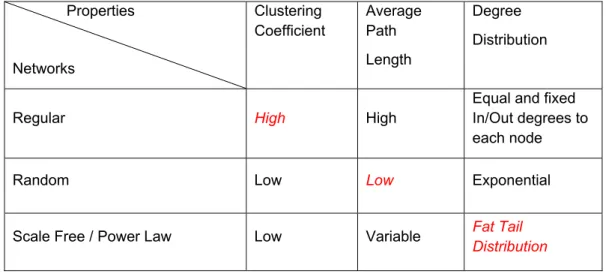
Like many real world socio-economic, communication, and information networks such as the www, financial networks are far from random and uncorrelated. In order to construct and characterize financial networks that have high concentration or localization of exposures with dense network interconnectivity between a few FIs, it is useful to briefly survey the well known classification of networks (see Table 2) and highlight the properties of small world networks that are a good fit for the financial network of exposures found in derivatives markets.19
The aim is to incorporate the highly skewed connectivity of 26 broker-dealers representing high concentration of derivatives liabilities in Table 1. This implies that other participants who are in the majority have little or no links to one another and instead are linked to the central core. Thus, a core-periphery structure (Borgatti and Everett, 1999) with small world network properties manifests itself in the derivatives network. This has also been regarded to be a statistical signature of complex social systems (Watts(1998) and Watts and Strogatz (1999)) namely, a top tier multi-hub of few agents who are highly connected among themselves (often called rich club dynamics) and to some other nodes in the periphery who show few if any connections amongst themselves. The properties of small world
networks and how contagion propagates through them will be briefly contrasted with that for
19 Small world networks are named after the work of Stanley Milgram (1967) on the six degrees of separation in
social networks. It has been found that globally, on average, everybody is linked to everybody else by no more than six indirect links.
the Erdös-Renyi random graph and also the Barabási and Albert (1999) scale free networks. In order to construct a network for financial derivatives that shows dominance of few players with a 92 percent and upwards of concentration of derivatives exposures to one another, use will be made of network statistics and dynamics described below regarding high clustering, preferential attachment in link formation, and identification of members with high ‘rich club’ statistics.
Networks are mainly characterized by a set of network statistics. These are: (i) the
probability of any two randomly selected nodes in a network being connected is denoted by p with there being total of N(N-1) possible links for directed graphs and N(N-1)/2 for
undirected graphs; (ii) measure of local interconnectivity between nodes called clustering coefficient (i denotes the clustering coefficient for node i and is the clustering coefficient for the network); (iii) the shortest path length of the network estimates the average shortest path between all pairs of randomly selected nodes; and (iv) degree distribution that gives the probability distribution P(k) as a function of the degrees k of each of the nodes, and p(k) gives the probability that a randomly selected node as exactly k links. The average number links per node is given by <k> = kk p(k) and the variance of links <k2> = kk2p(k). Where empirical sample data is used, p(k) = Nk/N-1 where Nkis the number of nodes with k links. Textbook prototypes of regular, random, and scale-free networks have properties in respect to the network statistics given in Table 2. As will be explained, small world networks
described by elements along the diagonal of Table 2 have one property in common with each of the other network types.
In Erdös-Renyi random networks in which connectivity between any two nodes is uncorrelated, the probability distribution of degrees is given by:
P(k) = 1 1 ! . (3)
The exact solution to the last term above is achieved in the limit when N→∞. The Erdös-Renyi random networks show little local interconnectivity or clustering. They have short path lengths due to the random link formation. The average shortest path between any two
arbitrarily chosen nodes is found to be “small” and bounded by the logarithm of the total number of nodes in the system.
Clustering in networks measures how interconnected each agent’s neighbours are and is considered to be the hallmark of social and species-oriented networks. Specifically, there should be an increased probability that two of an agent’s neighbours are also
neighbours of one another. For each agent with ki neighbours the total number of all possible directed links between them is given by ki(ki-1). Let Ei denote the actual number of links between agent i’s ki neighbors, viz. those of i’s ki neighbours who are also neighbours.
Table 2. Networks Statistics: Diagonal Elements Characterize Small World Networks
Source: Developed by author.
The clustering coefficient i for agent i is given by:20
i = ) 1 ( i i i k k E and = N N i i
1 . (4)The second term which gives the clustering coefficient of the network as a whole is the average of all i’s. Note that the clustering coefficient for an Erdös-Renyi random graph is
random = p. This is because in a random graph the probability of node pairs being connected by edges are by definition independent, so there is no increase in the probability for two agents to be connected if they were neighbours of another agent than if they were not. A high clustering coefficient for the network corresponds to high local interconnectedness and of a number of agents who operate as hubs in the core. In regular networks (see Table 2), all nodes have the same number of links to and from them, and they show high and local clustering but do not have short path lengths. Scale-free networks have highly skewed distribution of links that follows a power law in the tails of the degree distribution, i.e., the probability of a node possessing k degrees is given by
p(k) = , (5)
where >0 is called the power law exponent. Hence, there are some nodes which are very highly connected and many that are not. To generate power law statistics for nodes either in
20 Numerically, E
i, the connected edges is calculated as follows. Using the NxN adjacency matrix X = (aij)N with aij=1 (aij1 ,
for short) if there is a link between i and j and aij=0, if not. Agent i’s ki neighbors i = { j , ji, aij = 1} , Ei for a directed
graph is calculated as E =
i i j m jm a 1 , jm. Properties Networks Clustering Coefficient Average Path Length Degree DistributionRegular High High
Equal and fixed In/Out degrees to each node
Random Low Low Exponential
Scale Free / Power Law Low Variable Fat Tail
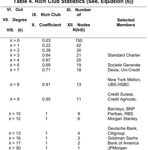
terms of their size or the numbers of links to/from them, Barabási and Albert (B-A,1999) proposed a process called preferential attachment, whereby nodes acquire size or numbers of links in proportion to their existing size or connectivity. 21 However, as noted by Zhou and Mondragon (2003) the growth dynamic of the B-A algorithm means that, while highly connected ‘rich’ nodes get richer, it does not follow that they could themselves preferentially connect to one another. An important discovery that was made by Watts (1998) and Watts and Strogatz (1999) with regard to social networks is that while, small world networks like scale-free networks have in-egalitarian degree distribution with some very highly connected nodes, the central tiering of highly clustered nodes that work as hubs for the peripheral nodes (who have few direct connections to others in the periphery) is a signature feature only of small worlds. The hubs also facilitate short path lengths between two peripheral nodes. Therefore, unless there is a modification of the B-A algorithm as suggested by Zhou and Mondragon (2003) to allow for preferential attachment or assortative mixing among the nodes with large number of out degreesand not just a preference for high degree nodes (disassortative mixing) by low degree nodes, the combined core-periphery structure with the high clustering of small world networks with the characteristics given in Table 2 will not occur. Hence, the premise behind the modified B–A algorithm will be adopted to get the extreme concentration of bilateral exposures between SIFIs in the derivatives markets. Apart from the clustering coefficient, two further statistics will be used to characterize networks that show high concentration of activity. The first is the rich club coefficient. The rich club coefficient, k) is used to identify highly connected nodes that form the club characterized by a fully connected network (Colizza et. al.(2006)). The latter yields a coefficient of 1 and k# will denote the critical number of out-degrees the nodes need to have to be part of the largest sized richclub with k) = 1. The rich club coefficient is estimated as:
k) = . (6)
Here N>k refers to the number of nodes with degrees higher than a given value of k and E>k denotes the number of connected edges among the N>k nodes. The denominator divided by two gives the maximum number of possible edges in any direction as in an undirected graph.
21 In the B–A preferential attachment algorithm, a node i receives a new link with probability p
i = ∑ . In
contrast, the Watts and Strogatz algorithm for the construction of small world networks, starts with a regular graph and then has random reconnections for a subset of out degrees of each node. This obtains the short path length and retains high clustering of the regular graph, but fails to obtain the scale free degree distribution with a few very highly connected nodes. Hence, following Zhou and Mondragon (2003), in this paper it is the B-A algorithm that is modified to achieve the core-periphery network with small world properties.
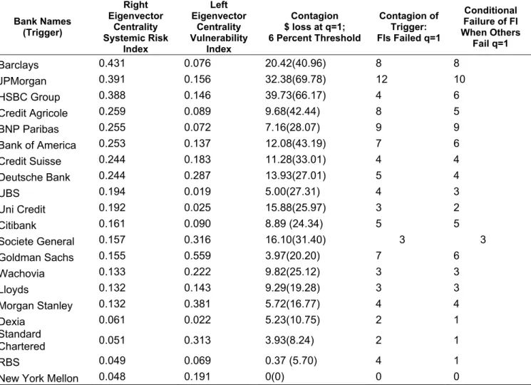
The network centrality measure that has been found by the author to correlate best with the capacity of a FI to cause the largest contagion losses on others in the Furfine (2003) type stress test is its eigenvector centrality statistic obtained for matrix in equation (2). The algorithm that determines it assigns relative centrality scores to all nodes in the network based on the principle that connections to high-scoring nodes contribute more to the score of the node in question than equal connections to low-scoring nodes. Denoting as the right eigenvector centrality for the ith node for matrix , the centrality score is proportional to the sum of the centrality scores of all nodes to which it is connected (i.e., ki neighbours). Hence, = ∑ . (7)
For the centrality measure in (7), the largest eigenvalue, λmax , and its associated eigenvector are taken. The ith component of this eigenvector then gives the centrality score of the ith node in the network. Using vector notation, the eigenvalue equation for the matrix in (2) for the eigen-pair (λmax, ) is given as:
= λmax . (8.a) Note that for a non-negative matrix in (2) with real entries, λmax is a real positive number and the eigenvector associated with the largest eigenvalue has non-negative components by the Perron-Frobenius theorem (see Meyer (2000), Chapter 8). Positive values for the centralities of all nodes of matrix in (2) are guaranteed by Perron-Frobenius theorem only if in (2) is irreducible.22 For matrix clearly, given equation (7), those nodes in the periphery with no out-degrees will have zero eigenvector centrality.
Finally, from the perspective of the measure of systemic risk, the so called right eigenvector of matrix given above in (8.a), as will be discussed, is what matters. A FI’s systemic risk index will be based on this. It measures the impact of FIs’ total liabilities relative to the respective capital of each of its counterparties given by the row sums of matrix in (2) on the stability of the system characterized by the maximum eigenvalue. The so-called dual left eigenvector, on the other hand, gives the impact of the exposures of each FI to others and hence can be seen to yield vulnerability indices. The left eigenvector of denoted by v1 is defined as
v1 = ´v1 = λmax v1. (8.b)
22 The condition of the Perron-Frobenius theorem that guarantees a positive eigenvector corresponding to the
maximum eigenvalue for the non-negative matrix is that the directed graph it represents should be irreducible. That is, for any randomly selected pairs of nodes (i,j) there is a path between them, viz. is strongly connected, Meyer (2000).
Note both the left and right eigenvectors yield the same maximum eigenvalue for the matrix
in (2).23
D. Economics Literature on Financial Networks
Pre-2007 financial network models in the economics literature have yielded mixed results. An influential and early work on connectivity in a financial network and that of financial contagion is that of Allen and Gale (2001). They gave rise to a mistaken view that follows only in the case of homogenous graphs, i.e., increasing connectivity
monotonically increases system stability in the context of diversification of counterparty risk.24 Battiston et al. (2010) have correctly shown that connectivity and stability of a network
is not a simple monotonic relationship but that beyond a point, connectivity in a network could increase instability. However, Battiston et al. (2010) do not offer insights into what sort of network topologies give rise to concerns about financial intermediaries being TITF either.
Indeed, the derivatives-based risk sharing networks, as discussed above, need to be
characterized by highly interconnected central tier composed of high degree hub nodes that have been called rich clubs. In contrast, the bulk of numerically based studies in financial contagion work (Nier et al. (2007) and Gai and Kapadia (2010)) has been confined to Erdös-Renyi random graphs and while they can be regarded as first steps, as financial networks are far from random, they have some way to go.
As little empirical work has been done to date on network structures of the specific markets underpinning off-balance sheet bank activity such as CDS responsible for triggering and propagating the 2007 crisis, it must be noted that the bulk of the empirical financial network approach has been confined to interbank credit markets for their role in the spread of financial contagion (see Furfine (2003) and Upper (2007)). However, the use of the entropy method (Upper and Worms (2004) and Boss et al. (2004)) for the construction of the matrix of bilateral obligations of banks that results in a complete and as homogenized
network structure as possible, greatly vitiates the potential for network instability or contagion.25
Recent work by Craig and von Peter (2010) using bilateral interbank data from
German banks and also by Fricke and Lux (2012) for the Italian interbank market has
23 Fujiwara et. al.(2009) have also noted the significance of the right and left eigenvectors to provide centrality
indices for banks and firms in a birpartite graph of lending relationships between banks and firms in Japan.
24 In a complete graph, if bank i’s total exposure is equally divided among its N-1 counterparties, then risk is
shared equally at the rate of 1/N-1. The demise of a single counterparty has a very small impact on i. In contrast, in the Allen and Gale (2001) incomplete circle network where each bank is exposed to only one other for the full 100 percent of its receivables, then the failure of any bank in the circle will bring the others down.
25 For a recent criticism of the entropy method in the construction of networks, see the 2010 ECB Report on Recent Advances in Modeling Systemic Risk Using Network Analysis.
identified thefollowing tiered core–periphery structure. They find that bilateral flow matrix (X), unlike in a complete network or as in a Erdös-Renyi random network, is sparse in the following way:
X =
. (9)
Here, CC stands for the financial flows among the core banks in the centre of the
network, CP stands for those between core and periphery banks, PC between periphery and core banks and PP stand for flows between periphery banks. The sparseness of the matrix relates to the fact that PP flows are zero and banks in the periphery of the network do not interact with one another. The localized clustering in the central core resembles the small world network property of being too interconnected and corresponds to the data-based CDS market network where this property was first identified in Markose et al. (2012). Hence, the criticism Craig and von Peter level at extant financial networks literature is worth stating here. They claim that many interbank models proposed in the economics literature (e.g., Allen and Gale (2000), Freixas et. al. (2000), and Leitner (2005)) ignore the tiered structure and do not analyze it in any rigorous way: “the notion that banks build yet another layer of intermediation between themselves goes largely unnoticed in the banking literature.” Craig and von Peter (2010) find that the tiered character of this market is highly persistent. This is similar to an outcome of competitive co-evolution ( Markose (2005)) in that to retain status quo in market shares, the core banks are hugely geared to the arms race involved there (see also Galbiati and Giansante (2010) and Giansante (2009)). Craig and von Peter (2010) go on to note that “the persistence of this tiered structure poses a challenge to interbank theories that build on Diamond and Dybvig (1983). If unexpected liquidity shocks were the basis for interbank activity, should the observed linkages not be as random as the shocks? Should the observed network not change unpredictably every period? If this were the case, it would make little sense for central banks and regulatory authorities to run interbank simulations gauging future contagion risks. The stability of the observed interbank structure suggests otherwise.” Fricke and Lux (2012) also report on the persistence of the central core structure in the overnight Italian interbank network of bilateral obligations that had about28 percent of all banks before the 2007 global financial crisis and 23 percent surviving afterwards.26 From the author’s experience of mapping the financial networks based on actual bilateral data of financial institutions for the Indian financial system, there appears to be a distinct variation in the core-periphery hierarchical structure noted by Craig and von Peter (2011) in the different types of financial activities. In their derivatives or contingent claims exposures and obligations, FIs show a far more marked concentration in the core both in terms of financial obligations and connectivity, with few FIs in the core and a large number of them in the periphery. In non-contingent claims-based borrowing and lending, the interbank market shows more diffusion in the core with a larger number of FIs in