NBER WORKING PAPER SERIES
CHANGING MONETARY POLICY RULES, LEARNING, AND REAL EXCHANGE RATE DYNAMICS
Nelson C. Mark Working Paper11061
http://www.nber.org/papers/w11061
NATIONAL BUREAU OF ECONOMIC RESEARCH 1050 Massachusetts Avenue
Cambridge, MA 02138 January 2005
An earlier version of this paper was presented at Mussafest, a conference in honor of Michael Mussa’s 60th birthday. I thank Mohan Kumar, Young-Kyu Moh, and seminar participants at the University of Auckland for useful comments. The views expressed herein are those of the author(s) and do not necessarily reflect the views of the National Bureau of Economic Research.
Changing Monetary Policy Rules, Learning, and Real Exchange Rate Dynamics Nelson C. Mark
NBER Working Paper No. 11061 January 2005
JEL No. F4
ABSTRACT
When central banks set nominal interest rates according to an interest rate reaction function, such as the Taylor rule, and the exchange rate is priced by uncovered interest parity, the real exchange rate is determined by expected inflation differentials and output gap differentials. In this paper I examine the implications of these Taylor-rule fundamentals for real exchange rate determination in an environment where market participants are ignorant of the numerical values of the model's coefficients but attempt to acquire that information using least-squares learning rules. I find evidence that this simple learning environment provides a plausible framework for understanding real dollar--DM exchange rate dynamics from 1976 to 2003. The least-squares learning path for the real exchange rate implied by inflation and output gap data exhibits the real depreciation of the 70s, the great appreciation (1979.4-1985.1) and the subsequent great depreciation (1985.2-1991.1) observed in the data. An emphasis on Taylor-rule fundamentals may provide a resolution to the exchange rate disconnect puzzle.
Nelson C. Mark
Department of Economics and Econometrics University of Notre Dame
Notre Dame, IN 46556 and NBER
Introduction
Understanding the macroeconomic determinants of the exchange rate has posed a chal-lenge to research ever since Meese and Rogo¤ (1983) reported the seemingly nonexistent relationship between macroeconomic fundamentals and the exchange rate. Although some progress has been made at econometrically modeling long-horizon exchange rate movements, the general failure of open economy macroeconomic theory— ranging from disequilibrium Keynesian models of Dornbusch (1976), Mussa (1982) and Obstfeld (1985) to the new open-economy macroeconomics of Obstfeld and Rogo¤ (1995)— to explain the exchange rate in terms of macro fundamentals has come to be known as theexchange rate disconnect puzzle [Obstfeld and Rogo¤ (2000)].1
In this paper, I provide evidence to suggest that the disconnect puzzle has resulted from focusing on the wrong set of fundamentals. Standard models predict that levels of variables such as domestic and foreign prices, money supplies, and income determine the exchange rate. While one strand of the literature attempts to model the disconnect between these fundamentals and the exchange rate[e.g., Devereux and Engel (2002), Kollman (2001), and Duarte and Stockman (2001)], I investigate the linkage of the exchange rate to an alternative set of fundamentals that arise when monetary policy is guided by a nominal interest rate reaction function commonly referred to as the ‘Taylor (1993) rule.’ The Taylor-rule approach predicts that the exchange rate is determined by relative expected in‡ation gaps and relative output gaps.
In the environment that I study, market participants do not know the exact Taylor-rule coe¢ cient values but attempt to acquire that information by least squares learn-ing.2 The learning model provides a plausible and useful framework for understanding observed real exchange rate dynamics over the post Bretton Woods ‡oat for the dollar-Deutschemark (DM) rate. The implied least-squares learning path displays many of the sizable and lengthy swings exhibited in the data–the depreciation of the late 1970s, the great appreciation of 1979.4–1985.1 and the subsequent great depreciation of 1985.2-1991.1.3 The choice of the dollar-deutschemark (DM) exchange rate is guided in part 1See Mark (1995), Mark and Sul (2001), Groen (2000,2002), and Rapach and Wohar (2002) who report econometric evidence on the long-horizon predictability of exchange rate returns from standard monetary model pricing errors.
2Lewis (1989a, b) conducts an analysis of Bayesian learning in the foreign exchange market to ex-amine the 1979 changes in the Fed’s operating procedures. She focused on shifts in the stochastic process governing monetary aggregates. In the monetary policy literature, Bullard and Mitra (2002) study conditions under which the rational expectations equilibrium is learnable while Orphanides (2003) examines whether the Fed’s imperfect knowledge of and attempts to learn the natural rate of unem-ployment responsible for the in‡ationary buildup of the 1970s.
3I adopt this terminology from Papell (2002). Engel and Hamilton (1990) referred to these ‡uc-tuations as ‘long-swings,’ while Frankel (1985) referred to dollar strength exhibited in the 80s as the
because the Bundesbank is one of the non-US central banks identi…ed by Clarida et. al. (1998) as having conducted monetary policy by following a variant of the Taylor rule.
This paper is part of a growing literature that recognizes the central role of interest rate reaction functions in exchange rate determination. Engel and West (2002) estimate the rational expectations time path of the real exchange rate implied by reaction function fundamentals and report a correlation of 0.4 between the implied rational expectations real dollar-DM rate and the historically observed real exchange rate from 1979 to 1998. In related work, Groen and Matsumoto (2004) calibrate a dynamic general equilibrium to the UK economy where monetary policy operates through interest rate reaction func-tions. The role of interest rate di¤erentials in the determination of the real exchange rate is not new and many strategies for modeling their dynamics have been employed to explain exchange rate dynamics with varying degrees of success. However, modeling the interest rate with the Taylor rule introduces a multivariate structure that produces a richer set of dynamics and interest rate forecasts that may be more accurate than those obtained from univariate time-series speci…cations.4
Modeling the learning process in exchange rate determination can be motivated by both general and speci…c considerations. From a general perspective, we not that in light of the poor track record of the macroeconomic rational expectations framework, it seems worthwhile to relax the strong informational assumptions that market participants already know the very structure that econometricians are struggling to learn. Both direct evidence of structural instability and indirect evidence through the inability of econometric exchange rate models to …t out of sample point to an important feature of the environment that should be explicitly accounted for.5 Adaptive learning schemes provide a plausible and straightforward strategy for modeling a public that must deal with a changing environment.
More speci…cally, a signi…cant change in the economic environment that is important to take into account is the change in central bank interest rate response to expected in‡ation that occurred with the appointment of Paul Volker to the Federal Reserve 4e.g., Frankel (1979), Meese and Rogo¤ (1988), Edison and Pauls (1993), Campbell and Clarida (1987), and Baxter (1994). Mark and Moh (2004) consider nonlinear (threshold) models for real interest rate di¤erentials and …nd that the implied rational expectations path for the real exchange rate has very little power to explain historical movements in the real exchange rate. For evidence on the importance of a multivariate approach, see Clarida and Taylor (1997) who show that information in the term structure of the forward premium provides signi…cant out-of-sample predictive power for the exchange rate.
5That is the Meese and Rogo¤ (1983) problem. See Cheung, Chinn and Pascual (2003) for a recent and nearly as discouraging assessment of the ability of econometric models to generate out-of-sample exchange rate predictions. My analysis does not suggest an out-of-sample forecasting experiment as a way to evaluate the model. Least squares learning, which itself is estimation with a recursively updated sample, is the standard method of generating out-of-sample forecasts. Since dozens of articles have shown this technique to be unable to signi…cantly improve over the random walk forecast, it is unlikely that we will be able to do so here, especially if the underlying coe¢ cient values are changing over time.
chairmanship in 1979. Clarida et. al. (2000) found that in the pre-1979 data, an increase in expected in‡ation led to a reduction in the real interest rate because the Fed typically reacted by raising the nominal interest rate by less than the increase in expected in‡ation. Following the appointment of Paul Volker as Chairman of the Federal Reserve System, they found the real interest rate to be increasing in expected in‡ation because the Fed now reacts by raising the nominal interest rate by more than the increase in expected in‡ation. When I estimate the central bank reaction functions in di¤erential form my estimates exhibit instability similar to that found in the Fed’s reaction function by Clarida et. al. The implied shift in the interest di¤erential reaction function is signi…cant in the pricing of the exchange rate because the shift fundamentally changes the relationship between the real exchange rate and national in‡ation di¤erentials.
The remainder of the paper is as follows. The next section describes the data. The least-squares learning exchange rate that I study is the outcome of agent’s attempts to learn the rational expectations real exchange rate priced by uncovered interest parity with interest rates determined by the Taylor rule. To set the stage for constructing the learning exchange rate paths, Section 2 reports estimates of the di¤erential in central bank’s interest rate reaction function under cross-country homogeneity of the response coe¢ cients. The empirical analysis of the real exchange rate is contained in Section 3. There, I begin with an examination of the estimated rational expectations real exchange rate. The model with learning is presented in subsection 3.2. Section 4 concludes.
1
The Data
The observations are quarterly and span from 1960.1 to 2003.3. The nominal exchange rate, German short-term nominal interest rates, GDP and potential GDP are from the OECD’s Economic Outlook. The imputed DM rate is used from 1998 to the end of the sample. Goods prices are measured by the real GDP de‡ator from the International Financial Statistics (series code 13499BIRZF). The U.S. Federal funds rate, GDP and potential GDP were obtained from FRED, the St. Louis Fed’s economic data web site. The output gap is de…ned as the percentage deviation of actual GDP from potential GDP. The availability of German potential GDP from source begins in 1966.1. These data are spliced together with the deviation from the Hodrick-Prescott (1997) (HP) trend to create a series that begins 1960.1. Quarterly in‡ation, the output gap and the nominal exchange rate return are stated in percent per annum. An increase in the real exchange rate signi…es a real depreciation of the dollar.
Figure 1 plots standardized values of the log real dollar-DM rate and the German– U.S. in‡ation di¤erential. The in‡ation di¤erential appears to be characterized by several distinct trends. From 1960 to 1979, rising relative US in‡ation generates a downward
Figure 1: German–U.S. in‡ation di¤erential and log real dollar–DM exchange rate
Figure 2: U.S.–German in‡ation di¤erential from 1960.2–1979.2, German–U.S. in‡ation di¤erential from 1979.3–2003.4, and log real dollar–DM exchange rate.
trend in the in‡ation di¤erential. The in‡ation di¤erential then increases from 1979 to 1992, declines from 1992 to 2000 and increases from 2000 through the end of the sample. The trends in the log real exchange rate coincides with that of the German-U.S. in-‡ation di¤erential in the post 1979 sample but the two series move in opposite directions in the pre 1979 sample, suggesting that a change in the relationship between the two series may have occurred at that time. Figure 2 allows for a regime change by plotting the US-German in‡ation di¤erential from 1960 to 1979 and the German-US di¤erential over the post 1979 sample. Allowing for this one-time regime change produces coincident trends in the real exchange rate and the in‡ation di¤erential.
Two preliminary conclusions can be drawn from this informal examination of the data. First, the …gures suggest shifting the emphasis on exchange rate determinants away from relative levels of macroeconomic fundamentals towards variables such as the di¤erences in di¤erences of national price levels may be a sensible thing to do. Second, impression one gets from the …gures is that the relationship between the real exchange rate trend and the in‡ation di¤erential changed around 1979. An obvious candidate for such a regime shift, is the change in the conduct of monetary policy. We now turn to an examination of the regime shift in the context of real exchange rate determination.
2
Di¤erentials in interest rate reaction functions
This section presents evidence to support modeling the interest di¤erential as a di¤eren-tial in monetary policy reaction functions under cross-country homogeneity restrictions on coe¢ cients for expected in‡ation and the output gap.Let German variables be denoted with a ‘star’ and let German-U.S. di¤erentials be denoted with a tilde. Then et = ( t t),eit = (it it), and xet = (xt xt) are German-U.S. di¤erentials in in‡ation, short-term nominal interest rates and output gaps, respectively.6 The log real exchange rate isq
t.
My speci…cation of the interest rate reaction functions draws on Clarida et. al. (1998, 2002). They estimated the Fed’s in‡ation response coe¢ cient to be less than 1 in the pre-Volker sample and to be greater than 1 in the post-Volker sample. The weak nominal interest rate response exhibited during the pre-1979 sample, meant that an increase in expected in‡ation caused the real interest rate to decline whereas in the post-1979 sample an aggressive interest rate response meant that an increase in expected in‡ation would cause an increase in the real interest rate. Clarida et. al. (1998) estimate monetary policy reaction functions for the Bundesbank and several other countries using data spanning from 1979 to 1993. They …nd that over this period, Bundesbank reactions
6Actual GDP lies above potential GDP whenx
to changes in in‡ation were similar to those of the post-1979 Fed.7
For my analysis, the Fed is assumed to set the deviation of its target for the Federal funds rateiT
t;from the desired leveliin response to the deviation of the public’s expected in‡ation from the target in‡ation rate (Et t+1 ); and the output gap xt; according to
iTt =i+ (Et t+1 ) + xxt; (1) where the central bank and the public employ the same model to forecast future in‡ation. The actual interest rate is subject to an exogenous and i.i.d. policy shock t;and is set according to a partial adjustment mechanism to re‡ect the central bank’s desire to limit interest rate volatility,
it= (1 )iTt + it 1+ t: (2) The Bundesbank is assumed to act in an analogous fashion. In addition, it may also react to nominal exchange rate deviations from its ‘natural level,’ which is given by purchasing-power parity. Clarida et. al. (1998) found that the feedback from the exchange rate to the German interest rate was statistically signi…cant but quantitatively very small. The German interest rate target is set by the rule,
itT =i + Et t+1 + xxt + sqt: (3) Imposing homogeneity on ( ; x) across countries gives the empirical speci…cation of the interest di¤erential,
eit = (1 )eiTt + eit 1+et; (4) eiTt = e+ Etet+1+ xxet+ sqt; (5) e i i ( ); (6) et iid (0; e2): (7)
To estimate the di¤erential in interest rate reaction functions, add and subtract
(1 ) et+1 on the right side of (4) and rearrange to obtain the regression
eit= + (1 ) [ et+1+ xext+ sqt] + eit 1+e0t; (8)
where = (1 ) ande0t=et (1 ) [et+1 Etet+1]. Under rational expectations,
the composite error terme0t is uncorrelated with date t information so(8) can be esti-mated by generalized method of moments (GMM ).8 The instrumental variables that I 7See also, Gerlach and Schnabel (1999) who estimate monetary policy reaction functions for an average of the EMU countries over a sample spanning from 1990 to 1998.
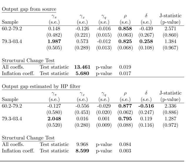
Table 1: Bundesbank–Fed Relative Interest-Rate Reaction Function Estimates by GMM
Output gap from source
x q J-statistic
Sample (s.e.) (s.e.) (s.e.) (s.e.) (s.e.) (p-value)
60.2-79.2 0.148 -0.126 -0.016 0.858 -0.439 2.571
(0.482) (0.221) (0.015) (0.063) (0.267) (0.860)
79.3-03.4 1.987 0.573 -0.012 0.825 0.258 1.384
(0.505) (0.289) (0.013) (0.068) (0.108) (0.967) Structural Change Test
All coe¤s. Test statistic 13.461 p-value 0.019 In‡ation coe¤. Test statistic 5.680 p-value 0.017 Output gap estimated by HP …lter
x q J-statistic
Sample (s.e.) (s.e.) (s.e.) (s.e.) (s.e.) (p-value)
60.2-79.2 -0.127 -0.556 -0.029 0.877 -0.516 2.336
(0.580) (0.453) (0.020) (0.062) (0.247) (0.886)
79.3-03.4 2.048 0.016 0.001 0.795 0.119 1.287
(0.520) (0.280) (0.009) (0.088) (0.116) (0.972) Structural Change Test
All coe¤s. Test statistic 9.968 p-value 0.084 In‡ation coe¤. Test statistic 8.599 p-value 0.003
employ are a constant, three lags of the in‡ation di¤erential, three lags of the output gap di¤erential, three lags of the nominal interest di¤erential, and one lag of the real exchange rate.
I estimate eq. (8) over pre- and post-1979 sub-samples with the split occurring on 1979.3 to conform to evidence reported by Clarida et. al. (2002). The results are reported in Table 1. The in‡ation response coe¢ cient is estimated to be less than 1 over the pre-1979 period and is estimated to be greater than 1 in the post-1979 period. The estimated output gap coe¢ cient has the wrong sign in the pre-1979 sample but is not statistically signi…cant. The estimated exchange rate response coe¢ cient is also not signi…cant. Hansen’s GMM test of the over identifying restrictions does not reject the speci…cation. The results are qualitatively similar for both constructions of the output gap.
The structural shift of the Fed’s interest rate reaction function reported in the lit-erature also appears to describe the reaction function di¤erential. To formally examine the evidence for a structural shift, I run Hodrick and Srivastava’s (1984) GMM-test for structural change.9 The hypothesis of no structural change in any of the coe¢ cients is strongly rejected when the output gap is constructed by the source agency and is marginally rejected when the output gap is estimated by the HP …lter. The hypothesis of no structural change in the in‡ation response coe¢ cient is strongly rejected for both constructions of the output gap.
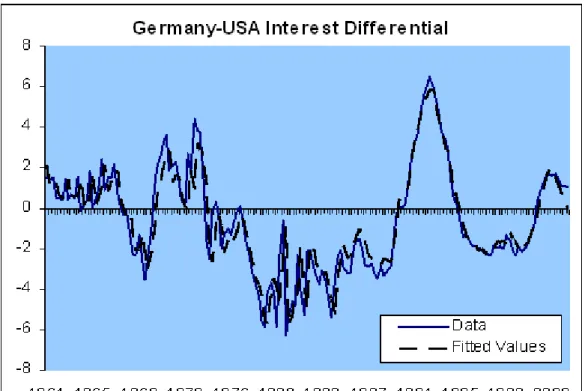
A visual account of the …t is provided in Figure 3 which plots the actual interest di¤erential and …tted values. In generating these …tted values, I employ forecasts of the in‡ation di¤erential generated by a fourth order bivariate autoregression in the in‡ation di¤erential and the output gap (from source agency) di¤erential. It can be seen that this simple speci…cation appears to work reasonably well in describing the dynamics of the interest di¤erential. Tractability in the ensuing analysis is facilitated by imposing coe¢ cient homogeneity in the interest rate rule across countries, and the estimation results suggest that imposing these restrictions is not unreasonable. Since the empirical analysis does not …nd that s is signi…cant, I set it to zero in the remainder of the analysis.
than 1 indicate that an increase in expected in‡ation elicits a weak response from the central bank that results in a reduction of the real interest rate which stimulates the economy, leading to a further increase in in‡ation. Values greater than 1 imply that the central bank responds aggressively to an increase in in‡ation by raising the nominal interest rate su¢ ciently to raise the real interest rate.
9The k dimensional coe¢ cient vector estimated from subsample j = 1;2 be b
j is has
asymp-totic distribution pTj bj j N(0; j): If the observations from the two subsamples are
in-dependent, then under null hypothesis of no structural change H0 : 1 = 1 the test statistic
HS = b1 b1 0 1 Tt +
2 T2
1
b1 b1 is asymptotically distributed as a chi-square variate with
Figure 3: Fitted values employ one-period ahead forecast of in‡ation di¤erential gener-ated from a fourth-order bi-variate autoregression for the in‡ation di¤erential and the output gap di¤erential.
3
An empirical model of the real exchange rate
Since the goal of the learning public is to discover the (minimum state variable) rational expectations equilibrium, I begin with a discussion of this case in subsection 3.1. In subsection 3.2, the model is extended to incorporate the public’s implementation of least-squares learning.3.1
Rational Expectations Real Exchange Rate
My primary aim is to study Taylor-rule fundamentals as determinants of real exchange rate movements. It is not to test a particular dynamic general equilibrium model. Thus, to model expectations formation, I adopting a relatively unstructured approach in the sense that the dynamics of the in‡ation di¤erential and the output gap di¤erential are taken to be exogenously generated from a bivariate vector autoregression (VAR). Market participants view this unrestricted VAR as the data generating process for in‡ation and the output gap which they use to construct forecasts of future in‡ation.
LetYe0
t = (et; : : : ;et p+1;ext; : : : ;xet p+1);andZevt0 = 1;Yet0 : The two-equationp th order VAR in regression form is,
et = b0 Zevt0 1+ev1t;
e
xt = b0xZevt0 1+ev2t;
which is convenient for estimation. For forecast generation, it is convenient to rewrite the VAR in companion form,
e
Yt = +AYet 1+evt:
To obtain the one-step ahead forecast of the in‡ation di¤erential, let e1 be the row
selection vector that has 1 as the (1;1) th element and zeros elsewhere such thatet=
e1Yet: SinceEtYet+1 = +AYet;we have
Etet+1 =e1 +AYet : (9) The output gap di¤erential can be recovered from the companion form of the VAR by de…ning the selection vectore2 that has 1 as the(1; p) th element and zeros elsewhere
such that
e
The log nominal exchange rate st; is priced by uncovered interest parity,
st =Etst+1+eit: (11) To price the real exchange rate, add and subtract Etet+1 from the right hand side of
(11) and rearrange to get
qt =Etqt+1+eit Etet+1: (12)
Substituting (4),(5), (9), and (10) into (12) gives
qt = Etqt+1+ [ + (1 ) ( 1)e1 ] (13)
+f(1 ) ( xe2+ e1A) e1AgYet+ eit 1+et:
Notice that the relationship between the expected real depreciation and the expected in‡ation di¤erential depends on the central bank’s in‡ation response coe¢ cient . The observed shift in the estimated response coe¢ cient suggests an explanation for the di-vergence between the trends in the real exchange rate and in‡ation di¤erentials in the pre-Volker sample and subsequent trend convergence. Because <1in the pre-Volker sample, a decline in the expected German-US in‡ation di¤erential led the public to ex-pect an increase in the German-US real interest di¤erential and a real depreciation of the dollar whereas with >1 in the post-1979 sample, a decline in the expected in‡ation di¤erential led the public to expect a decline in the German-US interest di¤erential and a real appreciation of the dollar.
With s= 0;forward iteration of real interest parity gives the real exchange rate as the undiscounted present value of expected future real interest di¤erentials.10 A rational expectations real exchange rate is the MSV solution
qt = 0+ 10Yt+ 2eit 1+ 3et; (14) where 2 = 1 ; (15) 3 = 1 1 ; (16) 0 1 = ([ xe2+ e1A] e1A) (I A) 1; (17) 0 = ( 01+ 2e1) (I A) 1 : (18)
10A solution exists provided that the real interest di¤erential has unconditional mean 0 which requires
The restriction on 0 ensures that the log real exchange rate has zero unconditional mean but because the price data are index numbers, the constant cannot be identi…ed in the empirical work and this restriction cannot be imposed.
3.1.1 Estimated Rational Expectations Real Exchange Rate Path
Here, I present the estimated rational expectations (RE) real exchange rate path using coe¢ cients ( ; ; x; ; A) estimated on the full sample with a known breakpoint at 1979.3. Market participants are thus assumed to have known about the regime change, the Taylor rule coe¢ cient values and the VAR coe¢ cient values under each regime. From these estimated coe¢ cients I obtain values for the exchange rate coe¢ cients in eqs. (15)-(17):11 It is worth pointing out that the implied real exchange rate path is generated entirely by the fundamentals data and does not directly depend on actual exchange rate observations.
It is well known that the real exchange rate behaves much di¤erently under a ‡exible exchange rate regime than it does under a …xed regime [e.g., Mussa (1986), Baxter and Stockman (1989)] and because exchange controls were in place in the 1960’s through the 1970s, the uncovered interest parity pricing model would not be expected to work well prior to the ‡oat. Since my primary objective is to understand the determination of the real exchange rate during the ‡oating rate period, I generate the implied rational expectations real exchange rate beginning in 1976.2. This particular date draws upon a suggestion by Hansen and Hodrick (1982). They argued that after the 1973 breakdown of the Bretton Woods system, the public had expected a return to some form of pegged exchange rates and that the ‡exible exchange rate regime only became fully credible after the IMF’s Articles on Exchange Rate arrangements were amended.
The estimated time path of the RE real dollar-DM rate are displayed in Figure 3.1.1. The observations are scaled to express exchange rate returns in percent per annum. Using the HP-…ltered output gap, the RE real exchange rate path shows only a very loose connection with the real exchange rate data. The implied RE real exchange rate generated with the source constructed output gaps fares better. This implied RE path misses the real dollar depreciation of the late 1970s but captures the real appreciation through the mid 1980s and the subsequent depreciation. The implied turning point occurs in 1984.2 whereas in the data it occurs in 1985.1. The implied exchange rate then depreciates from 1984.3 to 1992.2 whereas in the data, the depreciation more or less continues until 1995.3.
The implied RE depreciation from 1984 to 1992 is much larger than that observed in the data. This occurs in part because there was a one-time upward spike in relative Ger-11I employ a 4th order VAR for the in‡ation and output gap di¤erentials, which the BIC rule suggested was appropriate.
man in‡ation in 1991.1 that coincided with a negative value of the relative German-US output gap. Because the VAR coe¢ cients are estimated over the full sample, informa-tion about the spike is contained in these estimates. As time approaches 1991.1, agents are thus partially able to anticipate the spike. A large expected in‡ation di¤erential combined with a low output gap di¤erential leads people to expect, through the interest rate reaction function, an increase in the German interest di¤erential and a real dollar depreciation.
From 1994.1 to 1997.3, both the implied RE real exchange rate and the data show a gradual real dollar appreciation. The …nal turning point for the implied RE real exchange rate leads the data somewhat. The turning point for the RE path is at 1997.3 and for the data is at 2000.4.
The implied RE real exchange rates are substantially more volatile than the data. The sample standard deviation of the 1-quarter real exchange rate return in the data is 20.06 percent whereas the implied return volatility is 76.83 percent using the source constructed output gap and is 36.81 percent when using the HP …lter constructed output gap.
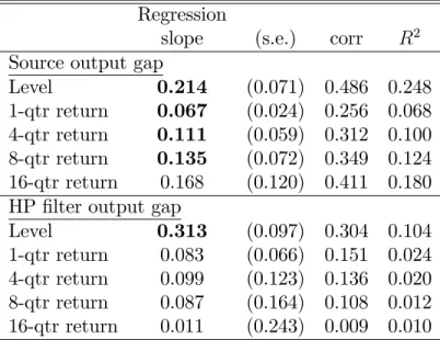
Table 2 quanti…es the co-movements between the implied RE real exchange rate path and the data. The table reports results from regressing the data on the estimated RE real exchange rate. I run the regressions both in log levels and in percent changes at 1, 4, 8, and 16 quarter horizons. The estimated slope coe¢ cients, regressionR2sand both the
short-and-long horizon return correlations exhibit systematic co-movements both in the level as well as in the changes between the estimated rational expectations fundamental
Table 2: Regressions of Real Exchange Rate Data on RE Rate
Regression
slope (s.e.) corr R2
Source output gap
Level 0.214 (0.071) 0.486 0.248
1-qtr return 0.067 (0.024) 0.256 0.068 4-qtr return 0.111 (0.059) 0.312 0.100 8-qtr return 0.135 (0.072) 0.349 0.124 16-qtr return 0.168 (0.120) 0.411 0.180 HP …lter output gap
Level 0.313 (0.097) 0.304 0.104
1-qtr return 0.083 (0.066) 0.151 0.024 4-qtr return 0.099 (0.123) 0.136 0.020 8-qtr return 0.087 (0.164) 0.108 0.012 16-qtr return 0.011 (0.243) 0.009 0.010
Notes: Bold face indicates signi…cance at the 5 percent level in a one-sided test. Newey and West (1987) standard errors. Correlation is denoted by corr.
real exchange rate and the actual exchange rate.12
3.2
Learning Dynamics
Unless strong assumptions are made about the knowledge held by market participants regarding the underlying economic environment, the analysis of the RE real exchange rate path begs the question as to whether the observed real exchange rate data over the ‡oat could have been generated by the model. I now relax some of these informational assumptions by setting market participants in a learning environment. Agents know the relevant functions so there is no model misspeci…cation but they do not know the parameter values in the policy rule or the coe¢ cient values in the VAR that governs 12My results are qualitatively similar to those reported in Engel and West (2002) who undertake a related analysis. There are several di¤erences between our analyses of the implied RE real dollar-DM rate. First, Engel and West work with a discounting model( s>0):Second, they equate the actual interest di¤erential to the target interest di¤erential eit=eiTt , whereas my analysis takes account
of central bank’s desire to smooth interest rate changes. Third, they impose parameter values for the interest rate reaction functions drawn from estimates reported in the literature whereas mine are estimated from the sample being studied. Fourth, they employ monthly data. They measure goods prices by the CPI and output with industrial production. Also, they construct their output gap as the residual from an output regression on a quadratic trend. Finally, they do not consider the implications of the Volker regime shift and begin their analysis in 1979 under assumption of a single …xed regime.
actual in‡ation di¤erentials and the output gap. In ‘real time,’ the public proceeds as a would-be econometrician who acquires knowledge of the relevant coe¢ cients using least-squares learning rules [Evans and Honkapojian (2001)].
The observations generated by the learning model are obtained as follows. At timet, using observations throught 1to obtain coe¢ cient values of the bivariate VAR on the in‡ation di¤erential and output gap di¤erential ( t 1; At 1); and the interest rate
re-action functions t 1; t 1; ;t 1; x;t 1 , beliefs about the nominal interest di¤erential
and expected in‡ation are formed as13
eit = t 1+ 1 t 1 ;t 1e1 t 1 (19)
+ 1 t 1 x;t 1e2+ ;t 1e1At 1 Yet+ t 1eit 1+et;
Etet+1 = e1 t 1+At 1Yet : (20)
Given coe¢ cient values 0t 1 = 0t 1; 01t 1; 2t 1; 3t 1 ; agent’s perceived law of mo-tion for the real exchange rate draws on the conjectured form of the ramo-tional expectamo-tions solution,
qt= 0t 1+ 01t 1Yet+ 2t 1eit 1+ 3t 1et: (21) The expected future real exchange rate is then obtained from the perceived law of motion,
Etqt+1 = 0t 1+ 01t 1 t 1+At 1Yet + 2t 1eit: (22)
The actual law of motion for the real exchange rate is obtained by substituting(20) (22)
into the real interest parity condition (12) which gives
qt= 0t+ 01tYet+ 2teit 1+ 3tet; (23) where 0t = 0;t 1+ 1;t 1 e1+ ;t 1 2;t 1+ 1 t 1+ 1 + 2;t 1 t 1; 0 1t = x;t 1e2+ 2;t 1 x;t 1e2+ ;t 1e1At 1 + ;t 1 1 e1+ 01;t 1 At 1; 2t = t 1 1 + 2;t 1 ; 3t = 1 + 2;t 1:
13Central banks know the monetary policy reaction functions. That is how they setei
t. The public
does not know the coe¢ cient values and must estimate them. The recursive least squares estimates of the policy reaction functions are used in the actual law of motion to account for the possibility that the policy rule itself has evolved over time. The analysis accounts for this possibility.
The coe¢ cients are then updated as follows: 1. For the VAR coe¢ cients,
Rv;t = Rv;t 1+gt Zevt 1Zevt0 1 Rv;t 1 ; (24) (b ;t; bx;t) = (b ;t 1; bx;t 1) +gtRvt1Zevt 1 h (et;xet) Zevt0 1(b ;t 1; bx;t 1) i ;(25) where gt is the gain. In standard recursive least-squares estimation, the gain is decreasing with gt = 1=t. Letting ( ; A) = C(b ; bx) be the mapping from the regression to companion form coe¢ cients, the VAR coe¢ cients are updated according to the rule, ( t; At) = C(b ;t; bx;t):
2. The monetary policy reaction function coe¢ cients are updated by letting 0 = ( ;(1 ) ;(1 ) x; )andZeit0 = 1;eet;ext;eit 1 ;whereeet =e1( t 1 +At 1Yt): Compactly restating the relative reaction function aseit= 0Zeit+et allows the up-dating to proceed according to,
Ri;t = Ri;t 1+gt Zei;t 1Zei;t0 1 Ri;t 1 ; (26)
t = t 1 +gtRi;t1 1Zei;t 1 eit 0t 1Zei;t 1 : (27)
3. The real exchange rate coe¢ cients are updated by letting Ze0
qt = 1;Yet0;eit 1;et and
Rq;t = Rq;t 1+gt Zeq;tZeq;t0 Rq;t 1 ; (28)
t = t 1+gtRq;t1 1Zeq;t qt 0t 1Zeq;t : (29) Notice that the implied learning path employs observations only on the Taylor-rule fundamentals and does not directly employ observations on the real exchange rate.
The following considerations were taken into account in parameterizing the gain func-tion. The standard declining gain (gt= 1=t) is appropriate if the public believes that there is a single time-invariant structure. In this case, the learning model converges to the rational expectations equilibrium under standard regularity conditions. On the other hand, if the public believes that a regime change occurred at datet0, then it make sense
to reset the gain at the time of the known break point(gt = 1=(t t0+ 1) for t t0). A third possibility is that the public understands that they are operating in a continually changing environment but they may not know when or if the regime changes have oc-curred. In this case, it makes sense to employ recursive least squares with a constant
gain speci…cation as in Orphanides and Williams (2003). Under a constant gain, the least squares coe¢ cients do not converge to …xed values.
The international …nance environment has been subject to several potential sources of parameter instability over the past three decades. In addition to the shift in monetary policy reaction functions discussed above, I allow for two additional sources of structural instability. These include the German reuni…cation (1990.3) and the breakdown of the European Monetary System following the 1992 crisis. To allow for the potential impor-tance of these events, I consider the following alternative speci…cations of the gain. Gain type 1: Constant gain with g = 0:02: This is the value assumed by Orphanides
and Williams (2003), who calibrated the gain to the expectations of professional forecasters.
Gain type 2: Decreasing gain gt = 1=t throughout the entire sample.
Gain type 3: Decreasing gain that is reset at 1979.3 to coincide with the change in monetary policy.
Gain type 4: Decreasing gain that is reset both at 1979.3 and at 1990.3, the time of German reuni…cation.
Gain type 5: Decreasing gain that is reset at 1992.3 to coincide with the European Monetary System crisis.
As in the analysis of the rational expectations path, I generate the implied learning real exchange rate beginning in 1976.2. Pre-sample observations during the ‡oat (begin-ning in 1973) are employed to estimate initial values of the least-squares coe¢ cients and associated moment matrices. The learning paths associated with the alternative gain speci…cations are qualitatively very similar. To avoid excessive clutter, Figure 4 plots the implied learning paths only for gain speci…cations 1,4, and 5 generated with the output gap de…ned by the source statistical agencies along with the exchange rate data.14 Each of the learning paths exhibit, in varying degrees, the real dollar depreciation in the late 1970s, the great appreciation observed in the …rst half of the 1980s and the subsequent great depreciation.
The learning paths exhibit real dollar depreciation from 1976 through 1981.1 whereas the turning point in the data is 1980.1. The learning path for gain type 5 shows the real 14The learning paths associated with gain speci…cations 2 and 3 are suppressed to reduce clutter on the graph. Learning paths with the output gap as the deviation from the HP trend are not presented. While the HP trend may be a reasonable retrospective detrending device, due to the truncation of the HP …lter at the endpoints of the sample, it is not appropriate to assume that the retrospectively constructed gap is what the public believed the output gap to have been at the time. To employ the
Figure 4: Implied learning paths and the data for the real dollar-DM rate for alternative gain speci…cations. Output gap constructed at source.
dollar appreciating through 1984.3, marking a turning point two quarters prior to that observed in the data (1985.1). From this point, the real value of the dollar in the data falls until 1988.1, gains for a year then more or less trends downward until 1995.2. The implied learning path trends with the data from 1985 but unlike the implied RE path does not exaggerate the depreciation of 1992.1.
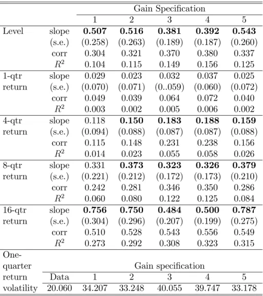
Table 3 reports regressions of the real exchange rate data on the alternative learning exchange rates. The correlation between the data in levels and the alternative implied learning exchange rates range from 0.304 (constant gain) to 0.380 (gain type 3). The correlations of quarterly rates of change range from 0.05 to 0.07 whereas the correlations of log changes at the 16 quarter horizon range from 0.51 to 0.56. In comparison to Table 2, it can be seen that the regressions on the implied RE real exchange rate exhibit higher R2 values but the slope coe¢ cients are smaller because the RE exchange rate is so much more volatile than the implied learning exchange rates. At short horizons, the RE depreciation exhibits higher correlation with the depreciation observed in the data, but the slope coe¢ cients are not signi…cant at longer horizons. This pattern is
reversed for the learning paths where the long-term trends are better explained by the learning model. Here, the slope coe¢ cients are not signi…cant at the 5 percent level in the 1-quarter depreciation regressions but are all signi…cant at the 16-quarter horizon.
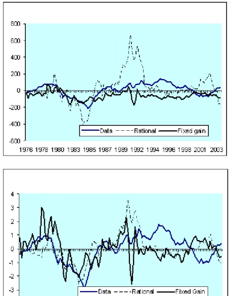
Figure 6 compares the estimated RE path, the constant gain learning path and the data. There are several di¤erences between the RE and the learning paths. First, the learning path produces real exchange rate volatility that is a much closer match to that in the data. Second, the learning path captures the 1976-1981 real dollar depreciation better than the estimated rational expectations path. Third, while both sets of estimates capture the great appreciation and the great depreciation of the 1980s, the estimated rational path predicts too much of a depreciation from 1985 to 1991 whereas the learning path predicts not enough of a depreciation. Both estimates exhibit the turning points in 1991.1 and 1991.3 found in the data. From about 1994 onwards, the qualitative dynamics of the estimated rational path and the learning path are not substantially di¤erent.
4
Conclusion
Standard open economy models predict that the exchange rate is determined by di¤er-ences in the levels of macroeconomic variables. The traditional focus on standard macro fundamentals in exchange rate determination has perhaps led to a rush of judgment about the irrelevance of macro-modeling of exchange rates. In contrast, the fundamen-tal determinants of the exchange rate are relative expected in‡ation gaps and relative output gaps when central banks conduct monetary policy by setting interest rates ac-cording to Taylor rules.
This paper has presented evidence that the real dollar-DM exchange rate is linked to Taylor rule fundamentals. I presented evidence that the interest di¤erential can be mod-eled as a di¤erential Taylor rule. Market participants were set in a learning environment where coe¢ cients of the Taylor rule changed over time. This simple framework provides a reasonably good macro-fundamentals driven explanation of the great appreciation and the subsequent great depreciation of the 1980s. While alternative approaches based on multiple equilibria (e.g., Flood and Rose (1999)) or micro market structure (Lyons and Evans (2003)) or are worthwhile avenues to pursue, the analysis in this paper suggests that additional work in the macroeconomic context is worthwhile.
Table 3: Regressions of the real dollar-DM rate on the implied learning real exchange rate in log levels and percent changes. Output gap constructed at source.
Gain Speci…cation 1 2 3 4 5 Level slope 0.507 0.516 0.381 0.392 0.543 (s.e.) (0.258) (0.263) (0.189) (0.187) (0.260) corr 0.304 0.321 0.370 0.380 0.337 R2 0.104 0.115 0.149 0.156 0.125 1-qtr slope 0.029 0.023 0.032 0.037 0.025 return (s.e.) (0.070) (0.071) (0..059) (0.060) (0.072) corr 0.049 0.039 0.064 0.072 0.040 R2 0.003 0.002 0.005 0.006 0.002 4-qtr slope 0.118 0.150 0.183 0.188 0.159 return (s.e.) (0.094) (0.088) (0.087) (0.087) (0.088) corr 0.115 0.148 0.231 0.238 0.156 R2 0.014 0.023 0.055 0.058 0.026 8-qtr slope 0.331 0.373 0.323 0.326 0.379 return (s.e.) (0.221) (0.212) (0.172) (0.173) (0.210) corr 0.242 0.281 0.346 0.350 0.286 R2 0.060 0.080 0.122 0.125 0.084 16-qtr slope 0.756 0.750 0.484 0.500 0.787 return (s.e.) (0.304) (0.296) (0.207) (0.199) (0.275) corr 0.510 0.528 0.543 0.556 0.549 R2 0.273 0.292 0.308 0.323 0.315
One-quarter Gain speci…cation
return Data 1 2 3 4 5
volatility 20.060 34.207 33.248 40.055 39.747 33.178
Notes: Bold face indicates signi…cance at the 5 percent level in a one-sided test. Newey and West (1987) standard errors. Correlation is denoted by corr.
Figure 5: Implied rational, learning, and actual real dollar-DM exchange rate.
Figure 6: Standardized values of implied rational, learning, and actual real dollar-DM exchange rate.
References
[1] Baxter, Marianne. “Real exchange rates and real interest di¤erentials: Have we missed the business-cycle relationship?”Journal of Monetary Economics33:1 (Feb-ruary 1994), 5-37.
[2] Baxter, Marianne and Alan Stockman, 1989. “Business cycles and the exchange-rate regime: Some international evidence,”Journal of Monetary Economics 23, (May 1989), 377-400.
[3] Bullard, James, and Kaushik Mitra. 2002. “Learning about Monetary Policy Rules,”
Journal of Monetary Economics, 49: 1105-1129.
[4] Campbell, John Y. and Richard Clarida. 1987. “The Dollar and Real Interest Rates,”Carnegie-Rochester Conference Series on Public Policy, 27, pp. 103-139. [5] Cheung, Yin-Wong, Menzie Chinn and Garcia Pascual. 2003. “Empirical Exchange
Rate Models of the Nineties: Are Any Fit to Survive?” Journal of International
Money and Finance, forthcoming.
[6] Clarida, Richard, Jordi Gali, and Mark Gertler. 2000. "Monetary Policy Rules and Macroeconomic Stability: Evidence and Some Theory." Quarterly Journal of
Economics, pp 147-180.
[7] Clarida, Richard, Jordi Gali, and Mark Gertler. 1998. "Monetary Policy Rules in Practice: Some International Evidence,"European Economic Review,42: pp. 1033-1067.
[8] Clarida, Richard and Mark P. Taylor. 1997. “The Term Structure of Forward Ex-change Premiums and the Forecastability of Spot ExEx-change Rates: Correcting the Errors,”Review of Economics and Statistics, 79(3):pp. 353-61.
[9] Devereux, Michael B. and Charles Engel. 2002. “Exchange Rate Pass-Through, Exchange Rate Volatility, and Exchange Rate Disconnect,”Journal of Monetary
Economics, pp. 913-940.
[10] Dornbusch, Rudiger. 1976. “Expectations and Exchange Rate Dynamics.”Journal
of Political Economy 84: pp. 1161–1176.
[11] Duarte, Margaride and Alan C. Stockman. 2001. “Rational Speculation and Ex-change Rates,”mimeo, Federal Reserve Bank of Richmond.
[12] Edison, Hallie and Dianne Pauls. “A Re-assessment of the Relationship between Real Exchange Rates and Real Interest Rates: 1974-1990,”Journal of Monetary Economics, 31(2), April 1993, 165-87.
[13] Engel, Charles and Kenneth D. West. 2002. “Taylor Rules and the Deutschemark-Dollar Real Exchange Rate,”mimeo, University of Wisconsin.
[14] Engel, Charles and James D. Hamilton. 1990. "Long Swings in the Dollar: Are They in the Data and Do Markets Know it?" American Economic Review, 80, pp. 689-713.
[15] Evans, George W. and Seppo Honkapohja. 2001. Learning and Expectations in
Macroeconomics, Princeton University Press, Princeton, NJ.
[16] Evans, Martin D.D. and Richard K. Lyons. 2003. "A New Micro Model of Exchange Rate Dynamics," NBER Working Paper 10379.
[17] Flood, Robert P. and Andrew K. Rose. 1999. "Understanding Exchange Rate Volatility without the Contrivance of Macroeconomics," Economic Journal.
[18] Frankel, Je¤rey. 1979. “On the Mark: A Theory of Floating Exchange Rates Based on Real Interest Di¤erentials,”American Economic Review, 69(4): 610-22
[19] Frankel, Je¤rey. 1985. "The Dazzling Dollar," Brookings Papers on Economic Ac-tivity 1, 199-217.
[20] Gerlach, Stefan and Gert Schnabel. 1999. "The Taylor Rule and Interest Rates in the EMU Area: A Note," BIS working paper No. 73.
[21] Groen, Jan J.J. 2002. “Cointegration and the Monetary Exchange Rate Model Revisited,”Oxford Bulletin of Economics and Statistics, 64, pp. 361-380.
[22] Groen, Jan J.J. 2000. “The Monetary Exchange Rate Model as a Long-Run Phe-nomenon,”Journal of International Economics, 52, 2.
[23] Groen, Jan J.J. and Akito Matsumoto. 2003. “Real Exchange Rate Persistence and Systematic Monetary Policy Behavior. mimeo Bank of England.
[24] Hansen, Lars P. and Robert J. Hodrick. 1983. “Risk Averse Speculation in the Foreign Exchange Market: An Econometric Analysis of Linear Models, in: J.A. Frenkel, ed., Exchange Rates and International Macroeconomics (University of Chicago Press, Chicago, IL).
[25] Hodrick, Robert J. and Edward C. Prescott. 1997. “Postwar U.S. Business Cycles: An Empirical Investigation ,”Journal of Money, Credit, and Banking.29: pp. 1–16. [26] Hodrick, Robert J. and Sanjay Srivastava. 1984. “An Investigation of Risk and Re-turn in Forward Foreign Exchange,”Journal of International Money and Finance, 3, pp. 5-29.
[27] Kollman, Robert. 2001. “Monetary Policy Rules in the Open Economy: E¤ects on Welfare and the Business Cycle.”mimeo University of Bonn
[28] Lewis, Karen K. 1989a. “Can Learning A¤ect Exchange-Rate Behavior? The Case of the Dollar in the Early 1980’s,”Journal of Monetary Economics, 23(1): 79-100 [29] Lewis, Karen K. 1989b. “Changing Beliefs and Systematic Rational Forecast Errors
with Evidence from Foreign Exchange,”American Economic Review, 79(4): 621-36 [30] Mark, Nelson C. 1995. “Exchange Rates and Fundamentals: Evidence on
Long-Horizon Predictability,”American Economic Review, 85,1, pp. 201-218.
[31] Mark, Nelson C. and Donggyu Sul. 2001. “Nominal Exchange Rates and Mone-tary Fundamentals: Evidence from a Small Post-Bretton Woods Panel,”Journal of International Economics, 53, pp. 29— 52.
[32] Mark, Nelson C. and Young-Kyu Moh. 2004. “What do Real Interest Di¤erentials Tell Us About the Real Exchange Rate? The Role of Nonlinearities,”mimeoTulane University.
[33] Meese, Richard and Kenneth Rogo¤. 1983. “Empirical Exchange Rate Models of the 1970’s: Do they Fit Out of Sample?”Journal of International Economics 14: pp. 3-24.
[34] Meese, Richard-A and Kenneth Rogo¤. 1988. “ Was It Real? The Exchange Rate-Interest Di¤erential Relation over the Modern Floating-Rate Period,”Journal of Finance, 43(4): 933-48
[35] Mussa, Michael. 1982. "A Model of Exchange Rate Dynamics,"Journal of Political Economy, 90(1): pp. 74-104.
[36] Mussa, Michael. 1986. “Nominal Exchange Rate Regimes and the Behavior of Real Exchange Rates: Evidence and Implications,”Carnegie Rochester Conference Se-ries on Public Policy, Autumn, 25, pp. 117-213.
[37] Newey, Whitney and Kenneth D. West. 1987. ‘A Simple, Positive Semi-de…nite, Heteroskedasticity and Autocorrelation Consistent Covariance Matrix,” Economet-rica, 55, pp. 703–708.
[38] Obstfeld, Maurice. 1985. “Floating Exchange Rates: Experience and Prospects.”
Brookings Papers on Economic Activity 2: pp. 369–450.
[39] Obstfeld, Maurice and Kenneth Rogo¤. 1995. “Exchange Rate Dynamics Redux.”
Journal of Political Economy 103: pp.624–660.
[40] Orphanides, Athanasios and John C. Williams. 2003. "The Decline of Activist Stabi-lization Policy: Natural Rate Misperceptions, Learning, and Expectations,"mimeo,
Federal Reserve Board.
[41] Papell, David. 2002. “The Great Appreciation, the Great Depreciation, and the Purchasing Power Parity Hypothesis,”Journal of International Economics, May, 51-82.
[42] Rapach, David and Mark Wohar. 2002. “Testing the Monetary Model of Exchange Rate Determination: New Evidence From A Century of data,”Journal of Interna-tional Economics, 58, pp. 359-385.
[43] Taylor, John. 1993. “Discretion versus Policy Rules in Practice,”Carnegie-Rochester Conference Series on Public Policy, 39, pp. 195-214.