Estimates and
Sample Sizes
7-1 Review and Preview7-2 Estimating a Population Proportion
7-3 Estimating a Population Mean: Known
7-4 Estimating a Population Mean: Not Known
7-5 Estimating a Population Variance
s s
Global warming is the increase in the mean temperature of air near the surface of the earth and the increase in the mean tempera-ture of the oceans. Scientists generally agree that global warming is caused by in-creased amounts of carbon dioxide, methane, ozone, and other gases that result from hu-man activity.
Global warming is believed to be respon-sible for the retreat of glaciers, the reduction in the Arctic region, and a rise in sea levels. It is feared that continued global warming will result in even higher sea levels, flooding, drought, and more severe weather.
Because global warming appears to have the potential for causing dramatic changes in our environment, it is critical that we recog-nize that potential. Just how much do we all recognize global warming? In a Pew Re-search Center poll, respondents were asked “From what you’ve read and heard, is there solid evidence that the average temperature on earth has been increasing over the past few decades, or not?” In response to that question, 70% of 1501 randomly selected adults in the United States answered “yes.” Therefore, among those polled, 70% believe in global warming. Although the subject mat-ter of this poll has great significance, we will focus on the interpretation and analysis of
the results. Some important issues that relate to this poll are as follows:
• How can the poll results be used to esti-mate the percentage of all adults in the United States who believe that the earth is getting warmer?
• How accurate is the result of 70% likely to be?
• Given that only 1501 225,139,000, or 0.0007% of the adult population in the United States were polled, is the sample size too small to be meaningful?
• Does the method of selecting the people to be polled have much of an effect on the results?
We can answer the last question based on the sound sampling methods discussed in Chapter 1. The method of selecting the peo-ple to be polled most definitely has an effect on the results. The results are likely to be poor if a convenience sample or some other nonrandom sampling method is used. If the sample is a simple random sample, the re-sults are likely to be good.
Our ability to understand polls and to in-terpret the results is crucial for our role as citizens. As we consider the topics of this chapter, we will learn more about polls and surveys and how to correctly interpret and present results.
> C H A P T E R P R O B L E M
How do we interpret a poll about global warming?
Review and Preview
In Chapters 2 and 3 we used “descriptive statistics” when we summarized data using tools such as graphs, and statistics such as the mean and standard deviation. We use “inferential statistics” when we use sample data to make inferences about population parameters. Two major activities of inferential statistics are (1) to use sample data to estimate values of population parameters (such as a population proportion or popula-tion mean), and (2) to test hypotheses or claims made about populapopula-tion parameters. In this chapter we begin working with the true core of inferential statistics as we use sample data to estimate values of population parameters. For example, the Chapter Problem refers to a poll of 1501 adults in the United States, and we see that 70% of them believe that the earth is getting warmer. Based on the sample statistic of 70%, we will estimate the percentage of alladults in the United States who believe that the earth is getting warmer. In so doing, we are using the sample results to make an infer-ence about the population.
This chapter focuses on the use of sample data to estimate a population parame-ter, and Chapter 8 will introduce the basic methods for testing claims (or hypotheses) that have been made about a population parameter.
Because Sections 7-2 and 7-3 use critical values,it is helpful to review this nota-tion introduced in Secnota-tion 6-2: denotes the zscore with an area of to its right. ( is the Greek letter alpha.) See Example 8 in Section 6-2, where it is shown that if
, the critical value is . That is, the critical value of has an area of 0.025 to its right.
z0.025 = 1.96 z0.025 = 1.96 a = 0.025 a a za 7-1
Estimating a Population Proportion
Key ConceptIn this section we present methods for using a sampleproportion to es-timate a population proportion. There are three main ideas that we should know and understand in this section.
•The sample proportion is the best point estimateof the population proportion. •We can use a sample proportion to construct a confidence intervalto estimate the
true value of a population proportion, and we should know how to interpret such confidence intervals.
•We should know how to find the sample size necessary to estimate a population proportion.
The concepts presented in this section are used in the following sections and chap-ters, so it is important to understand this section quite well.
Proportion, Probability, and Percent Although this section focuses on the population proportion p, we can also work with probabilities or percentages. In the Chapter Problem, for example, it was noted that 70% of those polled believe in global warming. The sample statistic of 70% can be expressed in decimal form as 0.70, so the sample proportion is . (Recall from Section 6-4 that p repre-sents the population proportion,and is used to denote the sample proportion.)
Point Estimate If we want to estimate a population proportion with a single value, the best estimate is the sample proportion Because consists of a single value, it is called a point estimate.
pN pN.
pN pN = 0.70 7-2
7-2 Estimating a Population Proportion 329
The sample proportion is the best point estimate of the population proportionp.
We use as the point estimate of pbecause it is unbiased and it is the most consistent of the estimators that could be used. It is unbiased in the sense that the distribution of sample proportions tends to center about the value of p; that is, sample propor-tions do not systematically tend to underestimate or overestimate p. (See Section 6-4.) The sample proportion is the most consistent estimator in the sense that the standard deviation of sample proportions tends to be smaller than the standard deviation of any other unbiased estimators.
pN pN
pN
pN
A point estimateis a single value (or point) used to approximate a popula-tion parameter.
Proportion of Adults Believing in Global Warming In the Chapter Problem we noted that in a Pew Research Center poll, 70% of 1501 randomly selected adults in the United States believe in global warming, so the sample proportion is . Find the best point estimate of the proportion of
all adults in the United States who believe in global warming.
Because the sample proportion is the best point estimate of the population proportion, we conclude that the best point estimate of pis 0.70. When using the sample results to estimate the percentage of all adults in the United States who believe in global warming, the best estimate is 70%.
Why Do We Need Confidence Intervals?
In Example 1 we saw that 0.70 was our bestpoint estimate of the population propor-tion p, but we have no indication of just how goodour best estimate is. Because a point estimate has the serious flaw of not revealing anything about how good it is, statisticians have cleverly developed another type of estimate. This estimate, called a
confidence intervalor interval estimate,consists of a range (or an interval) of values in-stead of just a single value.
pN = 0.70 1
A confidence interval(or interval estimate) is a range (or an interval) of values used to estimate the true value of a population parameter. A confi-dence interval is sometimes abbreviated as CI.
A confidence interval is associated with a confidence level, such as 0.95 (or 95%). The confidence level gives us the success rate of the procedure used to construct the confidence interval. The confidence level is often expressed as the probability or area (lowercase Greek alpha), where is the complement of the confidence level. For a 0.95 (or 95%) confidence level, For a 0.99 (or 99%) confidence level, a = 0.01.
a = 0.05. a
1 - a
The most common choices for the confidence level are 90% (with
95% (with and 99% (with The choice of 95% is most com-mon because it provides a good balance between precision (as reflected in the width of the confidence interval) and reliability (as expressed by the confidence level).
Here’s an example of a confidence interval found later (in Example 3), which is based on the sample data of 1501 adults polled, with 70% of them saying that they believe in global warming:
The 0.95 (or 95%) confidence interval estimate of the population propor-tion pis
It’s common for a media report to include a statement such as this: “Based on a Pew Research Center poll, the proportion of adults believing in global warming is esti-mated to be 70%, with a margin of error of 2 percentage points.” (We will discuss the margin of error later in this section.) Note that the confidence level is not mentioned. Although the confidence level should be given when reporting information about a poll, the media usually fail to include it.
Interpreting a Confidence Interval
We must be careful to interpret confidence intervals correctly. There is a correct inter-pretation and many different and creative incorrect interinter-pretations of the confidence interval
Correct: “We are 95% confident that the interval from 0.677 to 0.723 actu-ally does contain the true value of the population proportion p.” This means that if we were to select many different samples of size 1501 and construct the corresponding confidence intervals, 95% of them would actually contain the value of the population proportion p. (Note that in this correct interpretation, the level of 95% refers to the success rate of the processbeing used to estimate the proportion.)
Incorrect: “There is a 95% chance that the true value of p will fall between 0.677 and 0.723.” It would also be incorrect to say that “95% of sample proportions fall between 0.677 and 0.723.”
0.677 6 p 6 0.723.
0.677<p<0.723.
a = 0.01). a = 0.05),
a = 0.10),
The confidence levelis the probability (often expressed as the equiv-alent percentage value) that the confidence interval actually does contain the population parameter, assuming that the estimation process is repeated a large number of times. (The confidence level is also called the degree of confidence,or the confidence coefficient.)
1 - a
CAUTION
Know the correct interpretation of a confidence interval, as given above.
At any specific point in time, a population has a fixed and constant value p, and a confidence interval constructed from a sample either includes p or does not. Simi-larly, if a baby has just been born and the doctor is about to announce its gender, it’s incorrect to say that there is a probability of 0.5 that the baby is a girl; the baby is a girl or is not, and there’s no probability involved. A population proportion p is like the baby that has been born—the value of pis fixed, so the confidence interval limits ei-ther contain p or do not, and that is why it’s incorrect to say that there is a 95%
Curbstoning
The glossary for the Census defines curbstoning as“the practice by which a census enumerator fabricates a question-naire for a residence without actually visiting it.” Curbstoning occurs when a census enu-merator sits on a curbstone (or anywhere else) and fills out survey forms by making up responses. Because data from curbstoning are not real, they can affect the validity of the Census. The extent of curbstoning has been investigated in several studies, and one study showed that about 4% of Census enumerators prac-ticed curbstoning at least some of the time.The methods of Section 7-2 assume that the sample data have been collected in an appropriate way, so if much of the sample data have been obtained through curbstoning, then the re-sulting confidence interval estimates might be very flawed.
7-2 Estimating a Population Proportion 331
A confidence level of 95% tells us that the processwe are using will, in the long run, result in confidence interval limits that contain the true population proportion 95% of the time. Suppose that the true proportion of all adults who believe in global warming is . Then the confidence interval obtained from the Pew Research Center poll does not contain the population proportion, because the true population proportion 0.75 is not between 0.677 and 0.723. This is illustrated in Figure 7-1. Figure 7-1 shows typical confidence intervals resulting from 20 different samples. With 95% confidence, we expect that 19 out of 20 samples should result in confidence intervals that contain the true value of p, and Figure 7-1 illustrates this with 19 of the confi-dence intervals containing p, while one confidence interval does not contain p.
p = 0.75
0
.
65 This confidence interval does not contain p 0.75. 0.
70p 0
.
75 0.
800
.
85 Figure 7-1Confidence Intervals from 20 Different Samples
CAUTION
Confidence intervals can be used informally to compare different data sets, but the overlapping of confidence intervals should not be used for making formal and final conclu-sions about equality of proportions. (See “On Judging the Significance of Differences by Examining the Overlap Between Confidence Intervals,” by Schenker and Gentleman,
American Statistician,Vol. 55, No. 3.)
Critical Values
The methods of this section (and many of the other statistical methods found in the fol-lowing chapters) include reference to a standard zscore that can be used to distinguish between sample statistics that are likely to occur and those that are unlikely to occur. Such a zscore is called a critical value.(Critical values were first presented in Section 6-2, and they are formally defined below.) Critical values are based on the following observations:
1. Under certain conditions, the sampling distribution of sample proportions can be approximated by a normal distribution, as shown in Figure 7-2.
2. Azscore associated with a sample proportion has a probability of of falling in the right tail of Figure 7-2.
3. The zscore separating the right-tail region is commonly denoted by and is referred to as a critical valuebecause it is on the borderline separating zscores from sample proportions that are likely to occur from those that are unlikely to occur.
za>2, a>2 z⫽ 0 za/2 Found from Table A-2 (corresponds to area of 1 ⫺a/2) a/2 a/2 Figure 7-2 Critical Value in the Standard Normal Distribution zA/22
A critical valueis the number on the borderline separating sample statistics that are likely to occur from those that are unlikely to occur. The number is a critical value that is a zscore with the property that it separates an area of
in the right tail of the standard normal distribution (as in Figure 7-2). a>2
za>2 6308_Triola_ch07_p326-389.qxp 9/29/08 8:30 AM Page 331
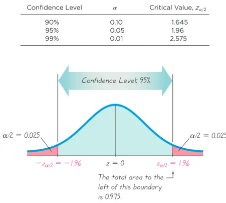
Confidence Level
:
95%The total area to the left of this boundary is 0.975.
Figure 7-3 Finding zA/22for a 95% Confidence Level
Margin of Error
When we collect sample data that result in a sample proportion, such as the Pew Research Center poll given in the Chapter Problem (with 70% of 1501 respondents believing in global warming), we can calculate the sample proportion . Because of random variation in samples, the sample proportion is typically different from the population proportion. The difference between the sample proportion and the popu-lation proportion can be thought of as an error. We now define the margin of error E
as follows.
pN
Confidence Level a Critical Value, za>2
90% 0.10 1.645
95% 0.05 1.96
99% 0.01 2.575
Finding a Critical ValueFind the critical value corre-sponding to a 95% confidence level.
A 95% confidence level corresponds to Figure 7-3 shows that the area in each of the red-shaded tails is We find by noting that the cumulative area to its left must be or 0.975. We can use technology or refer to Table A-2 to find that the area of 0.9750 (found in the bodyof the table) corresponds to z 1.96. For a 95% confidence level, the critical value is therefore To find the critical zscore for a 95% confidence level, look up 0.9750 (not0.95) in the body of Table A-2.
za>2 = 1.96. = 1 - 0.025, za>2 = 1.96 a>2 = 0.025. a = 0.05. za>2 2
Note:Many technologies can be used to find critical values. STATDISK, Excel, Minitab, and the TI-83 84 Plus calculator all provide critical values for the normal distribution.
Example 2 showed that a 95% confidence level results in a critical value of This is the most common critical value, and it is listed with two other common values in the table that follows.
za>2 = 1.96.
>
Nielsen Ratings
for College
Students
The Nielsen ratings are one of the most important mea-sures of television viewing,
and they affect bil-lions of dollars in televi-sion ad-vertising. In the past, the television viewing habits of college students were ig-nored, with the result that a large segment of the impor-tant young viewing audi-ence was ignored. Nielsen Media Research is now in-cluding college students who do not live at home. Some television shows have large appeal to view-ers in the 18–24 age bracket, and the ratings of such shows have increased sub-stantially with the inclusion of college students. For males, NBC’s Sunday Night Footballbroadcast had an increase of 20% after male college students were in-cluded. For females, the TV show Grey’s Anatomyhad an increase of 54% after fe-male college students were included. Those increased ratings ultimately translate into greater profits from charges to commercial sponsors. These ratings also give college students recognition that affects the programming they receive.
7-2 Estimating a Population Proportion 333
When data from a simple random sample are used to estimate a population proportion p, the margin of error,denoted by E,is the maximum likely difference (with probability , such as 0.95) between the observed sample proportion and the true value of the population proportion p. The margin of error Eis also called the maximum error of the estimateand can be found by multiplying the critical value and the standard deviation of sample proportions, as shown in Formula 7-1.
pN
1 - a
Formula 7-1 E = za>2 margin of error for proportions
A
pNqN
n
For a 95% confidence level, , so there is a probability of 0.05 that the sam-ple proportion will be in error by more than E. This property is generalized in the fol-lowing box.
a = 0.05
Objective
Construct a confidence interval used to estimate a population proportion.
3. There are at least 5 successes and at least 5 failures. (With the population proportions pand qunknown, we estimate their values using the sample proportion, so this requirement is a way of verifying that
and are both satisfied, so the normal distribu-tion is a suitable approximadistribu-tion to the binomial distri-bution. There are procedures for dealing with situa-tions in which the normal distribution is not a suitable approximation, as in Exercise 51.)
nq Ú 5
np Ú 5 Confidence Interval for Estimating a Population Proportion p
n = number of sample values pN = sample proportion p = population proportion
z score separating an area of in the right tail of the standard normal distribution
a>2
za>2 =
E = margin of error
Requirements
1.The sample is a simple random sample. (Caution:If the sample data have been obtained in a way that is not appropriate, the estimates of the population pro-portion may be very wrong.)
2.The conditions for the binomial distribution are satis-fied. That is, there is a fixed number of trials, the trials are independent, there are two categories of outcomes, and the probabilities remain constant for each trial. (See Section 5-3.)
Confidence Interval Notation
The confidence interval is often expressed in the following equivalent formats: or (pN - E, pN + E) pN ; E pN - E 6 p 6 pN + E where E = za>2 A pNqN n 6308_Triola_ch07_p326-389.qxp 9/29/08 8:30 AM Page 333
In Chapter 4, when probabilities were given in decimal form, we rounded to three significant digits. We use that same rounding rule here.
We now summarize the procedure for constructing a confidence interval estimate of a population proportion p:
Procedure for Constructing a Confidence Interval for p 1. Verify that the requirements are satisfied.
2. Refer to Table A-2 or use technology to find the critical value that corre-sponds to the desired confidence level.
3. Evaluate the margin of error
4.Using the value of the calculated margin of error Eand the value of the sample proportion find the values of the confidence interval limits and . Substitute those values in the general format for the confidence interval:
or
or
5. Round the resulting confidence interval limits to three significant digits. (Np - E, pN + E) pN ; E pN - E 6 p 6 pN + E pN + E pN - E pN, E = z a>22pNqN>n. za>2
Round-Off Rule for Confidence Interval Estimates of p
Round the confidence interval limits for pto three significant digits.
Constructing a Confidence Interval: Poll ResultsIn the Chapter Problem we noted that a Pew Research Center poll of 1501 randomly se-lected U.S. adults showed that 70% of the respondents believe in global warming. The sample results are , and .
a.Find the margin of error Ethat corresponds to a 95% confidence level. b.Find the 95% confidence interval estimate of the population proportion p. c.Based on the results, can we safely conclude that the majority of adults believe
in global warming?
d.Assuming that you are a newspaper reporter, write a brief statement that accu-rately describes the results and includes all of the relevant information.
REQUIREMENT CHECK We first verify that the necessary requirements are satisfied. (1) The polling methods used by the Pew Research Center result in samples that can be considered to be simple random samples. (2) The condi-tions for a binomial experiment are satisfied, because there is a fixed number of trials (1501), the trials are independent (because the response from one person doesn’t affect the probability of the response from another person), there are two categories of outcome (subject believes in global warming or does not), and the probability remains constant. Also, with 70% of the respondents believing in global warming,
pN = 0.70 n = 1501
7-2 Estimating a Population Proportion 335
the number who believe is 1051 (or 70% of 1501) and the number who do not be-lieve is 450, so the number of successes (1051) and the number of failures (450) are both at least 5. The check of requirements has been successfully completed.
a.The margin of error is found by using Formula 7-1 with (as found
in Example 2), and .
b.Constructing the confidence interval is quite easy now that we know the values of and E. We simply substitute those values to obtain this result:
This same result could be expressed in the format of or (0.677, 0.723). If we want the 95% confidence interval for the true population percentage,we
could express the result as .
c.Based on the confidence interval obtained in part (b), it does appear that the pro-portion of adults who believe in global warming is greater than 0.5 (or 50%), so we can safely conclude that the majority of adults believe in global warming. Because the limits of 0.677 and 0.723 are likely to contain the true population proportion, it appears that the population proportion is a value greater than 0.5. d.Here is one statement that summarizes the results: 70% of United States adults
believe that the earth is getting warmer. That percentage is based on a Pew Research Center poll of 1501 randomly selected adults in the United States. In theory, in 95% of such polls, the percentage should differ by no more than 2.3 percentage points in either direction from the percentage that would be found by interviewing all adults in the United States.
Analyzing Polls Example 3 addresses the poll described in the Chapter Problem. When analyzing results from polls, we should consider the following.
1. The sample should be a simple random sample, not an inappropriate sample (such as a voluntary response sample).
2. The confidence level should be provided. (It is often 95%, but media reports often neglect to identify it.)
3. The sample size should be provided. (It is usually provided by the media, but not always.)
4. Except for relatively rare cases, the quality of the poll results depends on the sampling method and the size of the sample, but the size of the population is usually not a factor.
67.7% 6 p 6 72.3%
0.70 ; 0.023
0.677 6 p 6 0.723
(rounded to three significant digits)
0.70 - 0.023183 6 p 6 0.70 + 0.023183 pN - E 6 p 6 pN + E pN E = z a>2A pNqN n = 1.96A (0.70)(0.30) 1501 = 0.023183 n = 1501 pN = 0.70, qN = 0.30, za>2 = 1.96 CAUTION
Never follow the common misconception that poll results are unreliable if the sample size is a small percentage of the population size. The population size is usually not a factor in determining the reliability of a poll.
Determining Sample Size
Suppose we want to collect sample data in order to estimate some population propor-tion. How do we know how manysample items must be obtained? If we solve the for-mula for the margin of error E(Formula 7-1) for n, we get Formula 7-2. Formula 7-2 requires as an estimate of the population proportion p, but if no such estimate is known (as is often the case), we replace by 0.5 and replace by 0.5, with the result given in Formula 7-3.
qN pN
pN
Objective
Determine how large the sample should be in order to estimate the population proportion p.
Notation
Finding the Sample Size Required to Estimate a Population Proportion
n = number of sample values pN = sample proportion p = population proportion
z score separating an area of in the right tail of the standard normal distribution
a>2
za>2 =
E = desired margin of error
Requirements
The sample must be a simple random sample of independent subjects. When an estimate is known: Formula 7-2
When no estimate is known: Formula 7-3 n =
[za>2]20.25 E2 pN n = [za>2]2pNqN E2 pN
If reasonable estimates of can be made by using previous samples, a pilot study, or someone’s expert knowledge, use Formula 7-2. If nothing is known about the
value of , use Formula 7-3.
Formulas 7-2 and 7-3 are remarkable because they show that the sample size does not depend on the size (N) of the population; the sample size depends on the desired confidence level, the desired margin of error, and sometimes the known estimate of . (See Exercise 49 for dealing with cases in which a relatively large sample is selected without replacement from a finite population.)
pN pN
pN
Round-Off Rule for Determining Sample Size
If the computed sample size nis not a whole number, round the value of nup to the next
largerwhole number.
How Many Adults Use the Internet? The Internet is af-fecting us all in many different ways, so there are many reasons for estimating the proportion of adults who use it. Assume that a manager for E-Bay wants to deter-mine the current percentage of U.S. adults who now use the Internet. How many adults must be surveyed in order to be 95% confident that the sample percentage is in error by no more than three percentage points?
7-2 Estimating a Population Proportion 337
a.Use this result from a Pew Research Center poll: In 2006, 73% of U.S. adults used the Internet.
b.Assume that we have no prior information suggesting a possible value of the proportion.
a.The prior study suggests that so (found from
With a 95% confidence level, we have so Also, the mar-gin of error is (the decimal equivalent of “three percentage points”). Because we have an estimated value of we use Formula 7-2 as follows:
We must obtain a simple random sample that includes at least 842 adults. b.As in part (a), we again use and , but with no prior
knowl-edge of (or ), we use Formula 7-3 as follows:
To be 95% confident that our sample percentage is within three percentage points of the true percentage for all adults, we should obtain a sim-ple random samsim-ple of 1068 adults. By comparing this result to the samsim-ple size of 842 found in part (a), we can see that if we have no knowledge of a prior study, a larger sample is required to achieve the same results as when the value of can be estimated.pN
n = [za>2]2
#
0.25 E2 = [1.96]2#
0.25 0.032 = 1067.1111 = 1068(rounded up) qN pN E = 0.03 za>2 = 1.96 n = [za>2]2pNqN E2 = [1.96]2(0.73)(0.27) 0.032 = 841.3104 = 842
(rounded up) pN E = 0.03 za>2 = 1.96. a = 0.05, qN = 1 - 0.73). qN = 0.27 pN = 0.73, CAUTION
Try to avoid these two common errors when calculating sample size:
1.Don’t make the mistake of using as the margin of error corresponding to “three percentage points.”
2.Be sure to substitute the critical zscore for For example, if you are working with 95% confidence, be sure to replace with 1.96. Don’t make the mistake of replacing za>2with 0.95 or 0.05.
za>2
za>2.
E = 3
Finding the Point Estimate and Efrom a Confidence Interval Sometimes we want to better understand a confidence interval that might have been obtained from a journal article, or generated using computer software or a calculator. If we al-ready know the confidence interval limits, the sample proportion (or the best point estimate) and the margin of error Ecan be found as follows:
Point estimate of p:
pN =
(upper confidence interval limit) + (lower confidence interval limit)
2
pN
Margin of error:
E =
(upper confidence interval limit) - (lower confidence interval limit)
2
The article “High-Dose Nicotine Patch Therapy,” by Dale, Hurt, et al. (Journal of the American Medical Association, Vol. 274, No. 17) in-cludes this statement: “Of the 71 subjects, 70% were abstinent from smoking at 8 weeks (95% confidence interval [CI], 58% to 81%).” Use that statement to find the point estimate and the margin of error E.
From the given statement, we see that the 95% confidence inter-val is . The point estimate is the value midway between the up-per and lower confidence interval limits, so we get
The margin of error can be found as follows:
Better-Performing Confidence Intervals
Important note:The exercises for this section are based on the method for construct-ing a confidence interval as described above, not the confidence intervals described in the following discussion.
The confidence interval described in this section has the format typically pre-sented in introductory statistics courses, but it does not perform as well as some other confidence intervals. The adjusted Wald confidence interval performs better in the sense that its probability of containing the true population proportion pis closer to the confidence level that is used. The adjusted Wald confidence interval uses this sim-ple procedure: Add 2 to the number of successes x, add 2 to the number of failures (so that the number of trials nis increased by 4), then find the confidence interval as described in this section. For example, if we use the methods of this section with
and , we get this 95% confidence interval: .
With and we use the adjusted Wald confidence interval by letting
and to get this confidence interval: . The
chance that the confidence interval contains pis closer to 95% than the chance that 0.281 6 p 6 0.719contains p.
0.300 6 p 6 0.700 0.300 6 p 6 0.700 n = 24 x = 12 n = 20 x = 10 0.281 6 p 6 0.719 n = 20 x = 10 E =
(upper confidence limit) - (lower confidence limit)
2
=
0.81 - 0.58
2 = 0.115
pN =
(upper confidence limit) + (lower confidence limit)
2 = 0.81 + 0.58 2 = 0.695 pN 0.58 6 p 6 0.81 pN 5
7-2 Estimating a Population Proportion 339
Another confidence interval that performs better than the one described in this sec-tion and the adjusted Wald confidence interval is the Wilson score confidence interval:
(It is easy to see why this approach is not used much in introductory courses.) Using and , the 95% Wilson score confidence interval is
For a discussion of these and other confidence intervals for p, see “Approximation Is Better than ‘Exact’ for Interval Estimation of Binomial Proportions,” by Agresti and Coull, American Statistician,Vol. 52, No. 2.
0.299 6 p 6 0.701. n = 20 x = 10 pN + za2>2 2n ; za>2Q pNqN + za2>2 4n n 1 + za2>2 n USING TECHNOL OG
Y
For Confidence Intervals
Select Analysis,then Confidence Intervals,
then Proportion One Sample,and proceed to enter the requested
items. The confidence interval will be displayed.
Select Stat, Basic Statistics,then 1 Proportion.In
the dialog box, click on the button for Summarized Data.Also click
on the Optionsbutton, enter the desired confidence level (the default
is 95%). Instead of using a normal approximation, Minitab’s default procedure is to determine the confidence interval limits by using an ex-act method. To use the normal approximation method presented in this
section, click on the Optionsbutton and then click on the box with
this statement: “Use test and interval based on normal distribution.” Use the Data Desk XL add-in that is a supplement to this book. First enter the number of successes in cell A1, then
en-ter the total number of trials in cell B1. Select DDXL,select
Confidence Intervals,then select Summ 1 Var Prop Interval (which is an abbreviated form of “confidence interval for a propor-tion using summary data for one variable”). Click on the pencil icon for “Num successes” and enter A1. Click on the pencil icon for “Num trials” and enter B1. Click OK. In the dialog box, select the
level of confidence, then click on Compute Interval.
Press STAT,select TESTS,then select
1-PropZIntand enter the required items. The accompanying display shows the result for Example 3. Like many technologies, the TI-83 84 calculator requires entry of the number of successes, so 1051 (which
> T I - 8 3 / 8 4 P L U S
E X C E L M I N I TA B S TAT D I S K
is 70% of the 1501 people polled) was entered for the value of x.
Also like many technologies, the confidence interval limits are ex-pressed in the format shown on the second line of the display.
TI-83 84 PLUS/
For Sample Size Determination
Select Analysis,then Sample Size
Determina-tion,then Estimate Proportion.Enter the required items in the di-alog box.
Sample size determination is not available as a built-in function
with Minitab, Excel, or the TI-83 84 Plus calculator.>
S TAT D I S K
Basic Skills and Concepts
Statistical Literacy and Critical Thinking
1. Poll Results in the MediaUSA Todayprovided a “snapshot” illustrating poll results from 21,944 subjects. The illustration showed that 43% answered “yes” to this question: “Would you rather have a boring job than no job?” The margin of error was given as percentage point. What important feature of the poll was omitted?
;1
7-2
2. Margin of ErrorFor the poll described in Exercise 1, describe what is meant by the state-ment that “the margin of error is percentage point.”
3. Confidence IntervalFor the poll described in Exercise 1, we see that 43% of 21,944 people polled answered “yes” to the given question. Given that 43% is the best estimate of the population percentage, why would we need a confidence interval? That is, what additional in-formation does the confidence interval provide?
4. SamplingSuppose the poll results from Exercise 1 were obtained by mailing 100,000 questionnaires and receiving 21,944 responses. Is the result of 43% a good estimate of the population percentage of “yes” responses? Why or why not?
Finding Critical Values.In Exercises 5–8, find the indicated critical z value. 5.Find the critical value that corresponds to a 99% confidence level.
6.Find the critical value that corresponds to a 99.5% confidence level.
7.Find for
8.Find for .
Expressing Confidence Intervals.In Exercises 9–12, express the confidence inter-val using the indicated format.
9.Express the confidence interval in the form of 10.Express the confidence interval in the form of 11.Express the confidence interval (0.437, 0.529) in the form of 12.Express the confidence interval in the form of
Interpreting Confidence Interval Limits.In Exercises 13–16, use the given confi-dence interval limits to find the point estimate and the margin of error E. 13.(0.320, 0.420) 14.
15. 16.
Finding Margin of Error.In Exercises 17–20, assume that a sample is used to es-timate a population proportion p. Find the margin of error E that corresponds to the given statistics and confidence level.
17. confidence
18. confidence
19.98% confidence; the sample size is 1230, of which 40% are successes.
20.90% confidence; the sample size is 1780, of which 35% are successes.
Constructing Confidence Intervals.In Exercises 21–24, use the sample data and confidence level to construct the confidence interval estimate of the population proportion p.
21. confidence
22. confidence
23. confidence
24. confidence
Determining Sample Size.In Exercises 25–28, use the given data to find the min-imum sample size required to estimate a population proportion or percentage. 25.Margin of error: 0.045; confidence level: 95%; and unknown
26.Margin of error: 0.005; confidence level: 99%; and unknown
27.Margin of error: two percentage points; confidence level: 99%; from a prior study, is
es-timated by the decimal equivalent of 14%.
28.Margin of error: three percentage points; confidence level: 95%; from a prior study, is
estimated by the decimal equivalent of 87%.
pN pN qN pN qN pN n = 5200, x = 4821, 99% n = 1236, x = 109, 99% n = 2000, x = 400, 95% n = 200, x = 40, 95% n = 500, x = 220, 99% n = 1000, x = 400, 95% 0.102 6 p 6 0.236 0.433 6 p 6 0.527 0.772 6 p 6 0.776 pN pN - E 6 p 6 pN + E. 0.222 ; 0.044 pN ; E. pN ; E. 0.720 6 p 6 0.780 pN ; E. 0.200 6 p 6 0.500 a = 0.02 za>2 a = 0.10. za>2 za>2 za>2 ;1
7-2 Estimating a Population Proportion 341
29. Gender SelectionThe Genetics and IVF Institute conducted a clinical trial of the XSORT method designed to increase the probability of conceiving a girl. As of this writing, 574 babies were born to parents using the XSORT method, and 525 of them were girls.
a.What is the best point estimate of the population proportion of girls born to parents using the XSORT method?
b. Use the sample data to construct a 95% confidence interval estimate of the percentage of girls born to parents using the XSORT method.
c. Based on the results, does the XSORT method appear to be effective? Why or why not?
30. Gender SelectionThe Genetics and IVF Institute conducted a clinical trial of the YSORT method designed to increase the probability of conceiving a boy. As of this writing, 152 babies were born to parents using the YSORT method, and 127 of them were boys.
a.What is the best point estimate of the population proportion of boys born to parents using the YSORT method?
b.Use the sample data to construct a 99% confidence interval estimate of the percentage of boys born to parents using the YSORT method.
c.Based on the results, does the YSORT method appear to be effective? Why or why not?
31. Postponing DeathAn interesting and popular hypothesis is that individuals can tem-porarily postpone their death to survive a major holiday or important event such as a birthday. In a study of this phenomenon, it was found that in the week before and the week after Thanksgiving, there were 12,000 total deaths, and 6062 of them occurred in the week before Thanksgiving (based on data from “Holidays, Birthdays, and Postponement of Cancer Death,” by Young and Hade, Journal of the American Medical Association,Vol. 292, No. 24.)
a.What is the best point estimate of the proportion of deaths in the week before Thanksgiv-ing to the total deaths in the week before and the week after ThanksgivThanksgiv-ing?
b.Construct a 95% confidence interval estimate of the proportion of deaths in the week be-fore Thanksgiving to the total deaths in the week bebe-fore and the week after Thanksgiving.
c.Based on the result, does there appear to be any indication that people can temporarily postpone their death to survive the Thanksgiving holiday? Why or why not?
32. Medical MalpracticeAn important issue facing Americans is the large number of med-ical malpractice lawsuits and the expenses that they generate. In a study of 1228 randomly se-lected medical malpractice lawsuits, it is found that 856 of them were later dropped or dis-missed (based on data from the Physician Insurers Association of America).
a.What is the best point estimate of the proportion of medical malpractice lawsuits that are dropped or dismissed?
b.Construct a 99% confidence interval estimate of the proportion of medical malpractice lawsuits that are dropped or dismissed.
c.Does it appear that the majority of such suits are dropped or dismissed?
33. Mendelian GeneticsWhen Mendel conducted his famous genetics experiments with peas, one sample of offspring consisted of 428 green peas and 152 yellow peas.
a.Find a 95% confidence interval estimate of the percentage of yellow peas.
b.Based on his theory of genetics, Mendel expected that 25% of the offspring peas would be yellow. Given that the percentage of offspring yellow peas is not 25%, do the results contra-dict Mendel’s theory? Why or why not?
34. Misleading Survey ResponsesIn a survey of 1002 people, 701 said that they voted in a recent presidential election (based on data from ICR Research Group). Voting records show that 61% of eligible voters actually did vote.
a. Find a 99% confidence interval estimate of the proportion of people who say that they voted.
b. Are the survey results consistent with the actual voter turnout of 61%? Why or why not? 6308_Triola_ch07_p326-389.qxp 9/29/08 8:30 AM Page 341
35. Cell Phones and CancerA study of 420,095 Danish cell phone users found that 135 of them developed cancer of the brain or nervous system. Prior to this study of cell phone use, the rate of such cancer was found to be 0.0340% for those not using cell phones. The data are from the Journal of the National Cancer Institute.
a. Use the sample data to construct a 95% confidence interval estimate of the percentage of cell phone users who develop cancer of the brain or nervous system.
b. Do cell phone users appear to have a rate of cancer of the brain or nervous system that is different from the rate of such cancer among those not using cell phones? Why or why not?
36. Global Warming PollA Pew Research Center poll included 1708 randomly selected adults who were asked whether “global warming is a problem that requires immediate ment action.” Results showed that 939 of those surveyed indicated that immediate govern-ment action is required. A news reporter wants to determine whether these survey results con-stitute strong evidence that the majority (more than 50%) of people believe that immediate government action is required.
a. What is the best estimate of the percentage of adults who believe that immediate govern-ment action is required?
b. Construct a 99% confidence interval estimate of the proportion of adults believing that immediate government action is required.
c. Is there strong evidence supporting the claim that the majority is in favor of immediate government action? Why or why not?
37. Internet UseIn a Pew Research Center poll, 73% of 3011 adults surveyed said that they use the Internet. Construct a 95% confidence interval estimate of the proportion of all adults who use the Internet. Is it correct for a newspaper reporter to write that “3 4 of all adults use the Internet”? Why or why not?
38. Job Interview MistakesIn an Accountemps survey of 150 senior executives, 47% said that the most common job interview mistake is to have little or no knowledge of the com-pany. Construct a 99% confidence interval estimate of the proportion of all senior executives who have that same opinion. Is it possible that exactly half of all senior executives believe that the most common job interview mistake is to have little or no knowledge of the company? Why or why not?
39. AOL Poll After 276 passengers on the Queen Elizabeth II cruise ship contracted a norovirus, America Online presented this question on its Internet site: “Would the recent outbreak deter you from taking a cruise?” Among the 34,358 people who responded, 62% an-swered “yes.” Use the sample data to construct a 95% confidence interval estimate of the pop-ulation of all people who would respond “yes” to that question. Does the confidence interval provide a good estimate of the population proportion? Why or why not?
40. Touch TherapyWhen she was nine years of age, Emily Rosa did a science fair experi-ment in which she tested professional touch therapists to see if they could sense her energy field. She flipped a coin to select either her right hand or her left hand, then she asked the therapists to identify the selected hand by placing their hand just under Emily’s hand without seeing it and without touching it. Among 280 trials, the touch therapists were correct 123 times (based on data in “A Close Look at Therapeutic Touch,” Journal of the American Med-ical Association,Vol. 279, No. 13).
a. Given that Emily used a coin toss to select either her right hand or her left hand, what proportion of correct responses would be expected if the touch therapists made random guesses?
b. Using Emily’s sample results, what is the best point estimate of the therapist’s success rate?
c. Using Emily’s sample results, construct a 99% confidence interval estimate of the propor-tion of correct responses made by touch therapists.
d. What do the results suggest about the ability of touch therapists to select the correct hand by sensing an energy field?
7-2 Estimating a Population Proportion 343
Determining Sample Size.In Exercises 41–44, find the minimum sample size re-quired to estimate a population proportion or percentage.
41. Internet UseThe use of the Internet is constantly growing. How many randomly se-lected adults must be surveyed to estimate the percentage of adults in the United States who now use the Internet? Assume that we want to be 99% confident that the sample percentage is within two percentage points of the true population percentage.
a. Assume that nothing is known about the percentage of adults using the Internet.
b. As of this writing, it was estimated that 73% of adults in the United States use the Internet (based on a Pew Research Center poll).
42. Cell PhonesAs the newly hired manager of a company that provides cell phone service, you want to determine the percentage of adults in your state who live in a household with cell phones and no land-line phones. How many adults must you survey? Assume that you want to be 90% confident that the sample percentage is within four percentage points of the true population percentage.
a. Assume that nothing is known about the percentage of adults who live in a household with cell phones and no land-line phones.
b. Assume that a recent survey suggests that about 8% of adults live in a household with cell phones and no land-line phones (based on data from the National Health Interview Survey).
43. Nitrogen in TiresA campaign was designed to convince car owners that they should fill their tires with nitrogen instead of air. At a cost of about $5 per tire, nitrogen supposedly has the advantage of leaking at a much slower rate than air, so that the ideal tire pressure can be maintained more consistently. Before spending huge sums to advertise the nitrogen, it would be wise to conduct a survey to determine the percentage of car owners who would pay for the nitrogen. How many randomly selected car owners should be surveyed? Assume that we want to be 95% confident that the sample percentage is within three percentage points of the true percentage of all car owners who would be willing to pay for the nitrogen.
44. Name Recognition As this book was being written, former New York City mayor Rudolph Giuliani announced that he was a candidate for the presidency of the United States. If you are a campaign worker and need to determine the percentage of people that recognize his name, how many people must you survey to estimate that percentage? Assume that you want to be 95% confident that the sample percentage is in error by no more than two per-centage points, and also assume that a recent survey indicates that Giuliani’s name is recog-nized by 10% of all adults (based on data from a Gallup poll).
Using Appendix B Data Sets.In Exercises 45–48, use the indicated data set from Appendix B.
45. Green M&M CandiesRefer to Data Set 18 in Appendix B and find the sample propor-tion of M&Ms that are green. Use that result to construct a 95% confidence interval estimate of the population percentage of M&Ms that are green. Is the result consistent with the 16% rate that is reported by the candy maker Mars? Why or why not?
46. Freshman 15 Weight GainRefer to Data Set 3 in Appendix B.
a. Based on the sample results, find the best point estimate of the percentage of college stu-dents who gain weight in their freshman year.
b. Construct a 95% confidence interval estimate of the percentage of college students who gain weight in their freshman year.
c. Assuming that you are a newspaper reporter, write a statement that describes the results. Include all of the relevant information. (Hint:See Example 3 part (d).)
47. Precipitation in BostonRefer to Data Set 14 in Appendix B, and consider days with precipitation values different from 0 to be days with precipitation. Construct a 95% confi-dence interval estimate of the proportion of Wednesdays with precipitation, and also con-struct a 95% confidence interval estimate of the proportion of Sundays with precipitation. Compare the results. Does precipitation appear to occur more on either day?
48. Movie RatingsRefer to Data Set 9 in Appendix B and find the proportion of movies with R ratings. Use that proportion to construct a 95% confidence interval estimate of the proportion of all movies with R ratings. Assuming that the listed movies constitute a simple random sample of all movies, can we conclude that most movies have ratings different from R? Why or why not?
Beyond the Basics
49. Using Finite Population Correction FactorIn this section we presented Formulas
7-2 and 7-3, which are used for determining sample size. In both cases we assumed that the population is infinite or very large and that we are sampling with replacement. When we have a relatively small population with size Nand sample without replacement, we modify Eto in-clude the finite population correction factorshown here, and we can solve for nto obtain the re-sult given here. Use this rere-sult to repeat Exercise 43, assuming that we limit our population to the 12,784 car owners living in LaGrange, New York, home of the author. Is the sample size much lower than the sample size required for a population of millions of people?
50. One-Sided Confidence IntervalA one-sided confidence intervalfor pcan be expressed
as or where the margin of error Eis modified by replacing with If Air America wants to report an on-time performance of at least x percent with 95% confidence, construct the appropriate one-sided confidence interval and then find the per-cent in question. Assume that a simple random sample of 750 flights results in 630 that are on time.
51. Confidence Interval from Small SampleSpecial tables are available for finding
con-fidence intervals for proportions involving small numbers of cases, where the normal distribu-tion approximadistribu-tion cannot be used. For example, given successes among trials, the 95% confidence interval found in Standard Probability and Statistics Tables and Formulae
(CRC Press) is . Find the confidence interval that would result if you were to incorrectly use the normal distribution as an approximation to the binomial distribu-tion. Are the results reasonably close?
52. Interpreting Confidence Interval LimitsAssume that a coin is modified so that it
favors heads, and 100 tosses result in 95 heads. Find the 99% confidence interval estimate of the proportion of heads that will occur with this coin. What is unusual about the results ob-tained by the methods of this section? Does common sense suggest a modification of the re-sulting confidence interval?
53. Rule of ThreeSuppose ntrials of a binomial experiment result in no successes.
Accord-ing to the Rule of Three,we have 95% confidence that the true population proportion has an upper bound of (See “A Look at the Rule of Three,” by Jovanovic and Levy, American Statistician,Vol. 51, No. 2.)
a. If nindependent trials result in no successes, why can’t we find confidence interval limits by
using the methods described in this section?
b. If 20 patients are treated with a drug and there are no adverse reactions, what is the 95%
upper bound for p, the proportion of all patients who experience adverse reactions to this drug?
54. Poll AccuracyA New York Timesarticle about poll results states, “In theory, in 19 cases
out of 20, the results from such a poll should differ by no more than one percentage point in either direction from what would have been obtained by interviewing all voters in the United States.” Find the sample size suggested by this statement.
3>n. 0.085 6 p 6 0.755 n = 8 x = 3 za. za>2 p 7 pN - E, p 6 pN + E E = za>2 A pNqN nA N - n N - 1
n = N pNqN[za>2]2 pNqN[za>2]2 + (N - 1)E2
7-2
7-3 Estimating a Population Mean: sKnown 345
Estimating a Population Mean: Known
Key ConceptIn this section we present methods for estimating a population mean. In addition to knowing the values of the sample data or statistics, we must also know the value of the population standard deviation, . Here are three key concepts that should be learned in this section.
1. We should know that the sample mean is the best point estimateof the popu-lation mean .
2. We should learn how to use sample data to construct a confidence intervalfor estimating the value of a population mean, and we should know how to inter-pret such confidence intervals.
3. We should develop the ability to determine the sample size necessary to esti-mate a population mean.
Important:The confidence interval described in this section has the requirement that we know the value of the population standard deviation , but that value is rarely known in real circumstances. Section 7-4 describes methods for dealing with realistic cases in which is not known.
Point Estimate In Section 7-2 we saw that the sample proportion is the best point estimate of the population proportion p. The sample mean is an unbiased esti-mator of the population mean , and for many populations, sample means tend to vary less than other measures of center, so the sample mean is usually the best point estimate of the population mean
The sample mean is the best point estimate of the population mean.
Although the sample mean is usually the bestpoint estimate of the population mean , it does not give us any indication of just how goodour best estimate is. We get more information from a confidence interval(or interval estimate), which consists of a range (or an interval) of values instead of just a single value.
Knowledge of The listed requirements on the next page include knowledge of the population standard deviation but Section 7-4 presents methods for estimat-ing a population mean without knowledge of the value of
Normality Requirement The requirements on the next page include the prop-erty that either the population is normally distributed or . If , the population need not have a distribution that is exactly normal. The methods of this section are robustagainst departures from normality, which means that these methods are not strongly affected by departures from normality, provided that those depar-tures are not too extreme. We therefore have a loose normality requirement that can be satisfied if there are no outliers and if a histogram of the sample data is not dra-matically different from being bell-shaped. (See Section 6-7.)
Sample Size Requirement The normal distribution is used as the distribu-tion of sample means. If the original populadistribu-tion is not itself normally distributed, then we say that means of samples with size have a distribution that can be approximated by a normal distribution. The condition is a common guideline, but there is no specific minimum sample size that works for all cases.
n 7 30 n 7 30 n … 30 n 7 30 s. s, S m x x m. x m x pN s s m x s
s
7-3 6308_Triola_ch07_p326-389.qxp 10/14/08 2:42 PM Page 345The minimum sample size actually depends on how much the population distrib-ution departs from a normal distribdistrib-ution. Sample sizes of 15 to 30 are sufficient if the population has a distribution that is not far from normal, but some other pop-ulations have distributions that are extremely far from normal and sample sizes greater than 30 might be necessary. In this book we use the simplified criterion of as justification for treating the distribution of sample means as a normal distribution.
Confidence Level The confidence interval is associated with a confidence level, such as 0.95 (or 95%). The confidence level gives us the success rate of the procedure used to construct the confidence interval. As in Section 7-2, is the complement of the confidence level. For a 0.95 (or 95%) confidence level, a = 0.05and za>2 = 1.96.
a n 7 30 Confidence Interval or or (x - E, x + E) x ; E x - E 6 m 6 x + E
where
E = za>2
#
s 2n ObjectiveConstruct a confidence interval used to estimate a population mean.
Notation
Confidence Interval for Estimating a Population Mean (with S Known)
population mean
population standard deviation sample mean
n = number of sample values = x = s = m
zscore separating an area of in the right tail of the standard normal distribution
a>2
za>2 =
E = margin of error
Requirements
1.The sample is a simple random sample.
2.The value of the population standard deviation is known.
s
3. Either or both of these conditions is satisfied: The pop-ulation is normally distributed or n 7 30.
Procedure for Constructing a Confidence Interval for (with Known ) 1. Verify that the requirements are satisfied.
2. Refer to Table A-2 or use technology to find the critical value that corre-sponds to the desired confidence level. (For example, if the confidence level is 95%, the critical value is za>2 = 1.96.)
za>2
S M
7-3 Estimating a Population Mean: sKnown 347
3. Evaluate the margin of error
4. Using the value of the calculated margin of error Eand the value of the sample mean find the values of the confidence interval limits: and
Substitute those values in the general format for the confidence interval:
or
or
5. Round the resulting values by using the following round-off rule. (x - E, x + E) x ; E x - E 6 m 6 x + E x + E. x - E x, E = z a>2
#
s>1nRound-Off Rule for Confidence Intervals Used to Estimate
1. When using the original set of datato construct a confidence interval, round the confidence interval limits to one more decimal place than is used for the original set of data.
2. When the original set of data is unknown and only the summary statistics
are used, round the confidence interval limits to the same number of decimal places used for the sample mean.
(n, x , s)
M
Interpreting a Confidence Interval As in Section 7-2, be careful to interpret confidence intervals correctly. After obtaining a confidence interval estimate of the population mean such as a 95% confidence interval of , there is a correct interpretation and many incorrect interpretations.
Correct: “We are 95% confident that the interval from 164.49 to 180.61 ac-tually does contain the true value of ” This means that if we were to select many different samples of the same size and construct the corresponding confidence intervals, in the long run 95% of them would actually contain the value of (As in Section 7-2, this cor-rect interpretation refers to the success rate of the processbeing used to estimate the population mean.)
Incorrect: Because is a fixed constant, it would be incorrect to say “there is a 95% chance that will fall between 164.49 and 180.61.” It would also be incorrect to say that “95% of all data values are between 164.49 and 180.61,” or that “95% of sample means fall between 164.49 and 180.61.” Creative readers can formulate other possible incorrect interpretations. m m m. m. 164.49 6 m 6 180.61 m,
Weights of MenPeople have died in boat and aircraft acci-dents because an obsolete estimate of the mean weight of men was used. In recent decades, the mean weight of men has increased considerably, so we need to update our estimate of that mean so that boats, aircraft, elevators, and other such devices do not become dangerously overloaded. Using the weights of men from Data Set 1 in Appendix B, we obtain these sample statistics for the simple random sample: and . Research from several other sources suggests that the population of weights of men has a standard deviation given by s = 26 lb.
x = 172.55 lb n = 40 1
Estimating
Wildlife
Population Sizes
The National ForestManagement Act protects endangered
species, includ-ing the north-ern spotted owl, with the result that the forestry industry was
not allowed to cut vast re-gions of trees in the Pacific Northwest. Biologists and statisticians were asked to analyze the problem, and they concluded that survival rates and population sizes were decreasing for the fe-male owls, known to play an important role in species survival. Biologists and statisticians also studied salmon in the Snake and Columbia Rivers in Wash-ington State, and penguins in New Zealand. In the arti-cle “Sampling Wildlife Pop-ulations” (Chance,Vol. 9, No. 2), authors Bryan Manly and Lyman McDonald com-ment that in such studies, “biologists gain through the use of modeling skills that are the hallmark of good statistics. Statisticians gain by being introduced to the reality of problems by biolo-gists who know what the crucial issues are.”
a.Find the best point estimate of the mean weight of the population of all men. b.Construct a 95% confidence interval estimate of the mean weight of all men. c.What do the results suggest about the mean weight of 166.3 lb that was used to
determine the safe passenger capacity of water vessels in 1960 (as given in the National Transportation and Safety Board safety recommendation M-04-04)?
REQUIREMENT CHECK We must first verify that the
re-quirements are satisfied. (1) The sample is a simple random sample. (2) The value of is assumed to be known with . (3) With , we satisfy the require-ment that “the population is normally distributed or .” The requirements are therefore satisfied.
a.The sample mean of 172.55 lb is the best point estimate of the mean weight for the population of all men.
b.The 0.95 confidence level implies that so (as was shown in Example 2 in Section 7-2). The margin of error Eis first calculated as follows. (Extra decimal places are used to minimize rounding errors in the confidence interval.)
With and , we now construct the confidence interval as follows:
c.Based on the confidence interval, it is possible that the mean weight of 166.3 lb used in 1960 could be the mean weight of men today. However, the best point estimate of 172.55 lb suggests that the mean weight of men is now considerably greater than 166.3 lb. Considering that an underestimate of the mean weight of men could result in lives lost through overloaded boats and aircraft, these results strongly suggest that additional data should be collected. (Additional data have been collected, and the assumed mean weight of men has been increased.)
The confidence interval from part (b) could also be expressed as or as (164.49, 180.61). Based on the sample with
and assumed to be 26, the confidence interval for the popu-lation mean is and this interval has a 0.95 confi-dence level. This means that if we were to select many different simple random samples of 40 men and construct the confidence intervals as we did here, 95% of them would actually contain the value of the population mean
Rationale for the Confidence Interval The basic idea underlying the con-struction of confidence intervals relates to this property of the sampling distribution of sample means: If we collect simple random samples of the same size n, the sample means are (at least approximately) normally distributed with mean mand standard
m. 164.49 lb 6 m 6 180.61 lb m s n = 40, x = 172.55 172.55 ; 8.06
164.49 6 m 6 180.61 (rounded to two decimal places as in x)
172.55 - 8.0574835 6 m 6 172.55 + 8.0574835 x - E 6 m 6 x + E E = 8.0574835 x = 172.55 E = za>2
#
s 1n = 1.96#
26 140 = 8.0574835 za>2 = 1.96 a = 0.05, n 7 30 n 7 30 s = 26 lb sCaptured Tank
Serial Numbers
Reveal
Popula-tion Size
During World War II, Allied intelligence specialists
wanted to determine the number of
tanks Germany was pro-ducing. Traditional spy tech-niques provided unreliable results, but statisticians ob-tained accurate estimates by analyzing serial numbers on captured tanks. As one example, records show that Germany actually produced 271 tanks in June 1941. The estimate based on serial numbers was 244, but tradi-tional intelligence methods resulted in the extreme esti-mate of 1550. (See “An Em-pirical Approach to Eco-nomic Intelligence in World War II,” by Ruggles and Brodie, Journal of the American Statistical Associ-ation,Vol. 42.)