Monetary and Fiscal Interactions without
Commitment and the Value of Monetary
Conservatism
∗
Klaus Adam
†Roberto M. Billi
‡ First version: September 29,2004Current version: April 28, 2005
Abstract
We study monetary andfiscal policy games in a dynamic sticky price economy where monetary policy sets nominal interest rates andfiscal pol-icy provides public goods financed with distortionary labor taxes. We compare the Ramsey outcome to non-cooperative policy regimes where one or both policymakers lack commitment power. Absence offiscal mitment gives rise to a public spending bias, while lack of monetary com-mitment generates the well-known inflation bias. An appropriately con-servative monetary authority can eliminate the steady state distortions generated by lack of monetary commitment and may even eliminate the distortions generated by lack offiscal commitment. The costs associated with the central bank being overly conservative seem small, but insuffi -cient conservatism may result in sizable welfare losses.
Keywords: optimal monetary andfiscal policy, sequential policy, dis-cretionary policy, time consistent policy, conservative monetary policy
JEL Classification: E52, E62, E63
1
Introduction
The difficulties associated with executing optimal but time-inconsistent policy
plans have received much attention following the seminal work of Kydland and Prescott (1977) and Barro and Gordon (1983). Time inconsistency problems, however, have hardly been analyzed in a dynamic setting where monetary and ∗We thank V.V. Chari, Ramon Marimon, Helge Berger, and seminar participants at
IGIER/Bocconi University for helpful discussions and suggestions. Errors remain ours. Views expressed reflect entirely the authors’ own opinions and not necessarily those of the European Central Bank.
†Corresponding author: European Central Bank, Research Department, Kaiserstr. 29,
60311 Frankfurt, Germany, [email protected]
fiscal policymakers are separate authorities engaged in a non-cooperative policy game. This may appear surprising given that the institutional setup in most developed countries suggests such an analysis to be of relevance.
In this paper we analyze non-cooperative monetary and fiscal policy games
assuming that policymakers cannot commit to future policy choices. We identify the policy biases emerging from sequential and non-cooperative decision making and assess the desirability of installing a central bank that is conservative in the
sense of Rogoff (1985). In other terms, we analyze the desirability of central
bank conservatism in a setting with endogenousfiscal policy.
Presented is a dynamic sticky price economy without capital along the lines
of Rotemberg (1982) and Woodford (2003) where output is inefficiently low due
to market power byfirms. The economy features two independent policymakers,
i.e., afiscal authority deciding about the level of public goods provision and a monetary authority determining the short-term nominal interest rate. Public goods generate utility for private agents and arefinanced by distortionary labor
taxes under a balanced budget constraint. Monetary andfiscal authorities are
assumed benevolent, i.e., maximize the utility of the representative agent. The natural starting point for our analysis is the Ramsey allocation, which
assumes full policy commitment and cooperation among monetary and fiscal
policymakers. The Ramsey allocation is second-best and thus provides a useful benchmark against which one can assess the welfare costs of sequential and non-cooperative policymaking.
In the presence of sticky prices and monopolistic competition monetary and
fiscal authorities both face a time-inconsistency problem. While price setters
are forward-looking, policymakers that decide sequentially fail to perceive the implications of their current policy decisions on past price setting decisions, since past prices can be taken as given at the time policy is determined. As a result,
policymakers underestimate the welfare costs of generating inflation today and
find it attractive to try to move output closer to itsfirst-best level. Sequential monetary policy, e.g., seeks to lower real interest rates so as to increase private consumption and output. Similarly, sequentialfiscal policy finds it optimal to increase output via increased spending on public goods.
We then characterize the non-cooperative Markov-perfect Nash equilibrium
where both policymakers determine their policies sequentially.1 To discover
the implications of relaxing monetary and fiscal commitment, it is useful to
proceed in steps. In particular, wefirst consider intermediate equilibria where one policymaker can commit while the other behaves in accordance with the reaction function that would be optimal in the Markov-perfect Nash equilibrium. These intermediate cases are self-confirming equilibria, rather than strict Nash
1Markov-perfect Nash equilibria are a standard refinement used in the applied dynamic
equilibria, but prove helpful for understanding the biases emerging in a situation
where both policymakers act sequentially.2 In addition, they provide natural
benchmarks for assessing the welfare gains from monetary conservatism. First, we consider an intermediate regime with sequentialfiscal policy (SFP) and monetary commitment. We show that, provided monetary policy imple-ments price stability, sequentialfiscal policy engages in excessive public spend-ing. Yet, thefiscal spending becomes less severe as inflation rises and this in-duces a fully committed monetary authority to allow for positive inflation rates.
This interaction between a commited monetary authority and a sequentialfiscal
authority indicates that an overly conservative central bank may potentially be harmful, since it amplifiesfiscal policy distortions.
We then consider the reverse situation with sequential monetary policy
(SMP) but time zero commitment by the fiscal authority. Sequential
mone-tary policy is shown to generate the familiar inflation bias. Since a reduction
in public spending can reduce the size of the monetary inflation bias, a
com-mittedfiscal authority deviates from the Ramsey solution in the self-confirming equilibrium by spending and taxing less.
Finally, we determine the Markov-perfect Nash equilibrium with sequential
monetary and sequential fiscal policy (SMFP). This equilibrium features an
inflation bias as well as a government spending bias, and tends to cause welfare losses that are considerably larger than in either the SFP or SMP regime. We then investigate whether a conservative central bank, that maximizes a weighted sum of an inflation loss term and the representative agent’s utility, is able to avoid the steady state welfare losses generated by sequential monetary policy. In models that abstract fromfiscal policy or in whichfiscal policy is exogenous, central bank conservatism has been shown to be an effective tool for eliminating
the policy biases generated by lack of monetary commitment, e.g., Rogoff(1985)
and Svensson (1997). We show that these results fully extend to a setting with endogenousfiscal policy. Moreover, with endogenousfiscal policy a conservative monetary authority may undo not only the distortions generated by lack of
monetary commitment but potentially also those stemming from lack offiscal
commitment.
More specifically, with sequential monetary and fiscal policy, an appropri-ate degree of monetary conservatism is found to recoup at least the losses from lack of monetary commitment. Welfare in the resulting Markov-perfect Nash equilibrium increases from the level associated with SMFP to that with SFP, or
even further. When fiscal policy is determined before monetary policy, a
con-servative monetary authority could even undo the steady state losses associated
2See Fudenberg and Levine (1993) or Sargent (1999) for an account of the concept of
with lack offiscal commitment. Sufficient monetary conservatism then approx-imately implements the Ramsey steady state, even though both policymakers lack commitment power.
Although determining the optimal degree of monetary conservatism might
be difficult in practice, we find the losses associated with suboptimal degrees
of conservatism to be fairly asymmetric. While an overly conservative central bank amplifies thefiscal spending bias, we find the associated welfare losses to be fairly small for the considered model calibrations. At the same time, the inflation bias associated with insufficient monetary conservatism gives rise to substantial welfare losses.
The remainder of this paper is structured as follows. After discussing the related literature in section 2, section 3 introduces the economic model and derives the implementability constraints. Section 4 presents the monetary and
fiscal policy regimes with and without commitment and analytically interprets
the steady state biases. After calibrating the model in section 5, section 6
provides a quantitative assessment of the steady state effects generated by the
various policy regimes under consideration. The case of a conservative central
bank is analyzed in section 7. A conclusion briefly summarizes the results and
provides an outlook for future work.
2
Related Literature
Problems of optimal monetary andfiscal policy are traditionally studied within
the optimal taxation framework introduced by Frank Ramsey (1927). In the
so-called Ramsey literature, monetary and fiscal authorities are treated as a
‘single’ authority and decisions are taken at time zero, e.g., Chari and Kehoe (1998). In seminal contributions, Kydland and Prescott (1977) and Barro and Gordon (1983) show that time zero optimal choices might be time-inconsistent, i.e., reoptimization in successive periods would suggest a different policy to be optimal than the one initially envisaged.
The monetary policy literature has extensively studies time-inconsistency
problems in dynamic settings and potential solutions to it, e.g., Rogoff(1985),
Svensson (1997) and Walsh (1995). However, in this literature fiscal policy
is typically absent or assumed exogenous to the model. Similarly, a number of contributions analyze sequentialfiscal decisions and the time-consistency of
optimal fiscal plans in dynamic general equilibrium models, e.g., Lucas and
Stokey (1983), Chari and Kehoe (1990) or Klein, Krusell, and Ríos-Rull (2004). This literature typically studies real models without money.
An important strand of the literature, developed by Sargent and Wallace
(1981), Leeper (1991), and Woodford (1998b), studies monetary andfiscal policy
literature, however, does not consider optimal policy and time-inconsistency problems, as it assumes policymakers to be fully committed to simple rules.
A range of papers discusses monetary andfiscal policy interactions with and
without commitment in a static framework where monetary andfiscal
policy-makers interact only once. Alesina and Tabellini (1987), e.g., consider a model where the monetary authority chooses the inflation rate and thefiscal
author-ity sets the tax rate to finance government expenditure. When policymakers
disagree about the trade-offbetween output and inflation, then monetary
com-mitment may not be welfare improving. Reduced seigniorage leads to increased
fiscal taxation and this might more than compensate the gains from reduced
inflation. Instead, our paper considers a cashless limit economy so abstracts
from seigniorage as a source of government revenue.
In a series of papers Dixit and Lambertini investigate the interaction between
monetary andfiscal policymakers with and without commitment. Namely, Dixit
and Lambertini (2001, 2003b) analyze the case of a monetary union but in a set-ting where the monetary authority does not face a time-inconsistency problem.
Dixit and Lambertini (2003a) consider a situation where monetary and fiscal
policymakers are both subject to a time-inconsistency problem. While thefiscal
authority maximizes social welfare, the monetary authority has a more conserv-ative output and inflation target and does not take into account the distortions
generated by fiscal policy instruments. In such a setting, monetary
commit-ment is ‘negated’ by sequentialfiscal policy, i.e., the equilibrium outcome with monetary commitment turns out to be the same as in the case with sequential monetary leadership.
This paper goes beyond these earlier contributions by studying a dynamic
model where current economic outcomes are influenced also by expectations on
future policy. Recently, Díaz-Giménez et al. (2004) study sequential monetary policy in a cash-in-advance economy with government debt. They consider a flexible price economy with exogenousfiscal spending and study the implications of indexed and nominal debt for monetary policy choices with and without
commitment. Interactions between monetary andfiscal policy in their model
operate through the government budget constraint and the seigniorage revenues raised by monetary policy. Our paper abstracts from seigniorage as a source of government revenue and instead considers the interactions arising from the presence of nominal rigidities.
3
The Economy
The next sections introduce a sticky price economy model, similar to the one studied in Schmitt-Grohé and Uribe (2004a), and derive the private sector equi-librium for given monetary andfiscal policy choices.
3.1
Private Sector
There is a continuum of identical households with preferences given by
E0 ∞
X t=0
βtu(ct, ht, gt) (1)
where ct denotes consumption of an aggregate consumption good, ht ∈ [0,1]
denotes the labor supply, andgt public goods provision by the government in
the form of aggregate consumption goods. Throughout the paper we impose the following conditions.
Condition 1 u(c, h, g) is separable in c, h, g and uc > 0, ucc < 0, uh < 0, uhh≤0,ug>0,ugg<0.
Each household produces a differentiated intermediate good. Demand for
that good is given by
ytd( e Pt Pt
)
whereytdenotes (private and public) demand for the aggregate good,Pte is the
price of the good produced by the household, andPtis the price of the aggregate good. The demand functiond(·)satisfies
d(1) = 1
∂d ∂(Pet/Pt)
(1) =η
whereη <−1denotes the elasticity of substitution between the goods of diff
er-ent households. The household choosesPte then hires the necessary amount of
laborehtto satisfy the resulting product demand, i.e.,
e
ht=ytd(Pte
Pt) (2)
Following Rotemberg (1982) we describe sluggish nominal price adjustment by assuming thatfirms face quadratic resource costs for adjusting prices according to θ 2( e Pt e Pt−1 −1)2
whereθ >0. Theflow budget constraint of the household is
Ptct+Bt=Rt−1Bt−1+Pt " e Pt Ptytdt( e Pt Pt)−wteht− θ 2( e Pt e Pt−1 −1)2 # +Ptwtht(1−τt) (3)
whereBtdenotes nominal bonds that pay BtRt in period t+ 1, wtis the real wage paid in a competitive labor market, andτtis a labor income tax.3
Although bonds are the only availablefinancial instrument, assuming
com-pletefinancial markets instead would make no difference for the analysis, since households have identical incomes in a symmetric price setting equilibrium. One should note that we also abstract from money holdings. This should be inter-preted as the ‘cashless limit’ of an economy with money, see Woodford (1998a). Money thus imposes only a lower bound on the gross nominal interest rate, i.e.,
Rt≥1 (4)
each period. Abstracting from money entails that we ignore seigniorage revenues generated in the presence of positive nominal interest rates. Given the size of these revenues in relation to GDP in industrialized economies, this does not
seem to be an important omission for the analysis conducted here.4
Finally, we impose a no Ponzi scheme constraint on household behavior, i.e.,
lim j→∞Et "Ãt+Yj−1 i=0 1 Ri ! Bt+j # ≥0 (5)
The household’s problem consists of choosing {ct, ht,eht,Pt, Bte }∞t=0 so as to maximize (1) subject to (2), (3), and (5) taking as given {yt, Pt, wt, Rt, gt, τt}. Using equation (2) to substituteeht in (3) and letting the multiplier on (3) be
λt/Pt, thefirst order conditions of the household’s problem are then equations (2), (3), and (5) holding with equality and also
uc(ct, ht, gt) =λt (6) uh(ct, ht, gt) =−λtwt(1−τt) (7) λt=βEtλt+1 Rt Πt+1 (8) 0 =λt µ ytd(rt) +rtytd0(rt)−wtytd0(rt)−θ(Πt rt rt−1 − 1) Πt rt−1 ¶ +βθEt ∙ λt+1( rt+1 rt Πt+1−1) rt+1 r2 t Πt+1 ¸
3Considering income or consumption taxes, instead, would be equivalent to a labor income
tax plus a lump sum tax (on profits). An earlier version of the paper, which is available upon request, considered the case with lump sum taxes.
4As emphasized by Leeper (1991), however, in a stochastic model seigniorage may
never-theless be an important marginal source of revenue. Since our paper abstracts from shocks, one can safely ignore this issue.
where
rt= Pte
Pt
denotes the relative price. Furthermore, there is the transversality constraint
lim j→∞Et µ βt+juc(ct+j, ht+j, gt+j) Bt+j Pt+j ¶ = 0 (9)
which has to hold each period.
3.2
Government
The government consists of two authorities, a monetary authority choosing
short-term nominal interest rates and afiscal authority deciding on government
expenditures and labor income taxes.
Government expenditures consist of spending related to the provision of
public goods gt and socially wasteful expenditure x that does not generate
utility for private agents. The level of public goods provision gt is a choice
variable, whilexis taken to be exogenous.
The government budget constraint is then given by
Bt Pt = Bt−1 Pt−1 Rt−1 Πt +gt+x−τtwtht
To simplify the analysis we eliminate government debt as a state variable by assuming that the government budget is balanced period-by-period and that
B−1= 0.5 The government budget constraint then reduces to
τtwtht=gt+x (10)
Importantly, the assumption of a balanced budget is not restrictive, since we
limit attention to the steady state of the economy. Assuming B−1 = 0,
how-ever, implies that we abstract from monetary andfiscal interactions that operate through the government budget constraint, as analyzed by Díaz-Giménez et al.
(2004). In particular, we ignore the monetary inflation bias arising from the
attempt to decrease the real value of outstanding government debt with ‘sur-prise’ inflation. Abstracting from nominal debt thus implies that we understate the size of the monetary inflation bias and the role for a conservative monetary
authority. In future work we plan to explore the effects of incorporating also
government debt dynamics.
We note that the absence of government debt could also be interpreted as
the fiscal authority not being able to commit to repay outstanding debt in
the future. Moreover, abstracting from debt insures that the no Ponzi scheme constraint (5) and the transversality constraint (9) are always satisfied.
3.3
Private Sector Equilibrium
In a symmetric equilibrium the relative price is given byrt= 1for allt. Using
the government budget constraint (10), thefirst order conditions of households
can be condensed into the following price setting equation
uc,t(Πt−1)Πt= uc,tht θ µ 1 +η+η µ uh,t uc,t − gt+x ht ¶¶ +βEt[uc,t+1(Πt+1−1)Πt+1] (11)
and a consumption Euler equation
uc,t Rt =βEt ∙ uc,t+1 Πt+1 ¸ (12) Conveniently, the previous equations do not make reference to taxes and real wages, while equations (6), (7), and (10) imply
τt= gt+xt gt+xt−htuuh,tc,t (13) wt= gt+xt ht − uh,t uc,t (14)
A rational expectations equilibrium is then a set of plans {ct, ht, Pt}
satis-fying equations (11) and (12) and also the feasibility constraint
ct+θ
2(Πt−1)
2+gt+x=ht (15)
given the policies{gt, Rt≥1}, the value ofx, and the initial conditionsB−1= 0 andP−1.
4
Monetary and Fiscal Policy Regimes
This section introduces the policy regimes analyzed in the remaining part of the paper. We consider policymakers that maximize the utility of the representative
agent. While the descriptive realism of this assumption is open to debate,
importantly it allows us to identify the inefficiencies generated by sequential
policy decisions.
4.1
Ramsey Policy
As a benchmark we consider the Ramsey equilibrium, which assumes
policymakers. The Ramsey equilibrium is second-best and given by the solution to the following maximization problem:
max {ct,ht,Πt,Rt,gt}∞t=0 E0 ∞ X t=0 βtu(c t, ht, gt) (16) s.t.
Equations(11),(12),(15)for allt Rt≥1for allt
The Ramsey planner thus maximizes the utility function of the representative agent subject to the implementability constraints (11) and (12), the
feasibil-ity constraint (15), and the lower bound on nominal interest rates.6 We thus
propose the following definition.
Definition 1 (Ramsey) A Ramsey equilibrium is a sequence{ct, ht,Πt, Rt, gt}∞t=0
solving problem (16).
Since optimal policy is time-inconsistent, the Ramsey equilibrium is initially
non-stationary. We will abstract from initial non-stationarities by defining a
Ramsey steady state as follows.
Definition 2 (Ramsey SS) Let{ct, ht,Πt, Rt, gt}∞
t=0be a Ramsey equilibrium,
then the Ramsey steady state is given bylimt→∞(ct, ht,Πt, Rt, gt).
One should note that the Ramsey steady state corresponds to the ‘timeless perspective’ commitment solution of Woodford (2003).
4.2
Sequential Policymaking
We now consider separate monetary andfiscal authorities that cannot commit
to future policy plans at time zero but rather decide upon policies at the time of implementation, i.e., period-by-period.
To facilitate the exposition we assume that a sequentially deciding policy-maker takes as given the current policy choice of the other policypolicy-maker as well as all future policy choices and future private sector choices. We prove the rationality of this assumption at the end of this section.
6The balanced budget constraint (10) and the initial condition B
−1 = 0are implicit in
the Phillips curve (11). The initial conditionP−1 can be ignored as it only normalizes the
4.2.1 Sequential Fiscal Policy
We consider here sequentialfiscal policymaking. Given the assumptions made
above, thefiscal authority’s maximization problem in periodt is:
max {ct+j,ht+j,Πt+j,gt+j} Et ∞ X j=0 βju(ct+j, ht+j, gt+j) (17) s.t.
Equations(11),(12),(15)for allt
Rt given
Et(ct+j, ht+j,Πt+j, gt+j, Rt+j) given forj≥1 Rt+j≥1for allj≥0
Eliminating Lagrange multipliers, the first order conditions associated with
problem (17) deliver thefiscal reaction function
1 ug,t = −1 uh,t 1 (1− Πt−1 2Πt−1η) ⎛ ⎝1− (Πt−1) ³ 1 +η+uh,t+htuhh,t uc,t η ´ 2Πt−1 ⎞ ⎠ (FRF)
Interestingly, forΠt= 1thefiscal reaction function simplifies to7
ug,t=−uh,t (18)
Thus, provided monetary policy implements price stability, discretionaryfiscal
policy equates the marginal utility of public consumption to the marginal disu-tility of work. Clearly, this leads to a suboptimally high level of public spending because condition (18) fails to take into account that
1. fiscal taxation has a negative wealth effect that crowds out private con-sumption;
2. public consumption isfinanced with labor income taxes, which distort the
labor supply decision.
Both of these effects are ignored by the fiscal authority, since the current monetary policy choice and all future choices are taken as given so the Euler equation (12) suggests that private consumption is determined. This makes it optimal to equate the marginal utility of public consumption to the marginal disutility of work.
The FRF also implies
∂(1/ug,t) ∂Πt
<0 (19)
7ForΠ
which shows that, ceteris paribus, the fiscal spending bias is less severe with positive inflation rates. For Πt > 1the marginal resource costs of generating
additional inflation through increasedfiscal spending fail to be zero, see equation (15). Fiscal policy takes these costs into account and reduces public spending correspondingly.8
The previous result suggests that a conservative monetary authority that implements price stability may increase the distortion generated by sequential
fiscal policy decisions. The distortions generated by monetary conservatism are
even larger, if monetary conservatism also leads to reduced labor input.
4.2.2 Sequential Monetary Policy
We now consider sequential monetary policy. Given the assumptions made
above, the monetary authority’s maximization problem in periodtis:
max {ct+j,ht+j,Πt+j,Rt+j} Et ∞ X j=0 βju(ct+j, ht+j, gt+j) (20) s.t.
Equations (11),(12),(15) for allt gt given
Et(ct+j, ht+j,Πt+j, gt+j, Rt+j) given forj≥1 (21)
Rt+j≥1for allj≥0 (22)
Eliminating Lagrange multipliers from the first order conditions delivers the
monetary reaction function
−uuc,t h,t µ 1 +η−2Πt−1 Πt−1 ¶ −η µ 1 +htuhh,t uh,t ¶ +2Πt−1 Πt−1 −ucc,tu c,t ∙ θ(Πt−1)Πt−ht µ 1 +η−gt+xt ht η zt ¶¸ = 0 (MRF)
Monetary policy sets the nominal interest rate Rt such that MRF is satisfied
each period. Appendix A.1 proves the following result
Lemma 1 Provided the discount factor β is sufficiently close to 1, satisfying MRF requires a strictly positive steady state inflation rate.
Sequential monetary policy generates the familiar inflation bias, e.g., Barro and Gordon (1983). Intuitively, monetary policy is tempted to stimulate de-mand by reducing interest rates. Since price adjustments are costly, the price
8For Π
t < 1 the fiscal bias is larger because higher fiscal spending increases inflation,
thereby reduces the resource costs of inflation. Interestingly, inflation could continue to have a moderating effect onfiscal spending as prices becomeflexible (θ→0). While the marginal costs of generating additional inflation decrease asθ→0, the Phillips curve (11) implies that any given increase in government spending generates larger and larger inflation.
level will not fully adjust to the demand increase. At the same time, nominal
wages areflexible and can increase so as to induce the additional labor supply
required to serve the demand increase. While the resulting real wage increase generates inflation, see the Phillips curve (11) and equation (14), the welfare costs of generating inflation are not fully taken into account, for reasons
dis-cussed before. Ultimately, monetary policy increases real wages and inflation
to the point where the marginal utility of an additional unit of consumption is equal to the marginal disutility of work and the perceived costs of inflation.
4.2.3 Sequential Monetary and Fiscal Policy
We are now in a position to define a Markov-perfect Nash equilibrium with
sequential monetary andfiscal policy (SMFP).
We first verify the rationality of our initial assumption that future choices can be taken as given. The private sector optimality conditions, (11) and (12), the feasibility constraint (15), as well as the policy reactions functions (FRF) and (MRF) all depend on current and future variables only. This suggests the existence of an equilibrium where current play depends on current and future economic conditions only and justifies taking as given future equilibrium play. If, in addition, monetary andfiscal policies are determined simultaneously each period, Nash equilibrium requires to take the other players’ decisions as given. This rationalizes all of our assumptions and provides the following definition.
Definition 3 (SMFP) A Markov-perfect equilibrium with sequential monetary andfiscal policy is a sequence{ct, ht,Πt, Rt, gt}∞t=0solving equations (11),(12),(15),
(FRF) and (MRF).
A steady state with SMFP is a stationary Markov-perfect equilibrium(c, h,Π, R, g). We now show that assuming Stackelberg leadership by one of the policy
authorities, instead of simultaneous decision making, does not affect the
equi-librium outcome.
While the policy problem of the Stackelberg follower remains unchanged, the Stackelberg leader must take into account the reaction function of the fol-lower and maximize over all policy choices. Importantly, however, the Lagrange
multipliers associated with imposing MRF on the sequentialfiscal problem (17)
or with imposing FRF on sequential monetary problem (20) are zero. This
fol-lows from the fact that these reaction functions can be derived from thefirst
order conditions of the leader’s policy problem even when the follower’s reaction function is not being imposed.
Intuitively, the leadership structure does not matter for the equilibrium
out-come because monetary and fiscal policymakers pursue the same objectives.
Differences to the Ramsey solution thus arise exclusively by relaxing the
policy interactions, and the sequence of moves, will matter only in section 7 when we introduce a central bank that is more inflation averse than the fiscal authority.
From Lemma 1 and the MRF, the steady state with sequential monetary andfiscal policy features an inflation bias, i.e.,Π>1. Whether there is also a positive fiscal spending bias depends on the severity of the inflation bias. For inflation rates close to one, public spending will be larger than in the Ramsey steady state, see the discussion in section 4.2.1; yet, for sufficiently high steady state inflation rates one cannot exclude that fiscal spending falls short of the Ramsey steady state level.
4.3
Intermediate Cases
As mentioned earlier, it is helpful to consider also intermediate cases where one policymaker can commit but the other behaves according to its sequential reaction function.
In the case with monetary commitment, the monetary authority internalizes
thefiscal reaction function (FRF). The monetary policy problem at time zero
is thus given by:
max {ct,ht,Πt,Rt,gt} E0 ∞ X t=0 βtu(ct, ht, gt) (23) s.t.
Equations (11),(12),(15),(FRF) for allt
Rt≥1for allt
We can provide the following definition.
Definition 4 (SFP) A self-confirming equilibrium with sequentialfiscal policy and monetary commitment is a sequence {ct, ht,Πt, Rt, gt}∞
t=0 solving problem
(23).
We note that the solution to problem (23) fails to be a Markov-perfect Nash equilibrium because the derivation of the FRF assumes thefiscal authority takes future monetary policy decisions as given. Under commitment the monetary authority, however, can condition current play on past play of thefiscal authority
and rationality requires the fiscal agent to take this fully into account.9 By
taking future play as given, the fiscal authority fails to correctly anticipate
the off-equilibrium behavior of monetary authority. At the same time, the
fiscal authority holds rational beliefs about equilibrium play, which implies that
9When the sequential authority is rational in this sence, it is easy to show that the
beliefs are never contradicted by outcomes. The solution to (23) is thus still a self-confirming equilibrium, see Fudenberg and Levine (1993) or Sargent (1999).
As in the Ramsey case, a steady state with sequentialfiscal policy (SFP) is
defined as the limit fort→ ∞of the self-confirming equilibrium with SFP.
Withfiscal commitment and sequential monetary policy (SMP),fiscal policy
anticipates the monetary reaction function and the policy problem at time zero is given by: max {ct,ht,Πt,Rt,gt} E0 ∞ X t=0 βtu(ct, ht, gt) (24) s.t.
Equations (11),(12),(15),(MRF) for allt
Rt≥1for allt
We thus have the following definition.
Definition 5 (SMP) A self-confirming equilibrium with sequential monetary policy andfiscal commitment is a sequence{ct, ht,Πt, Rt, gt}∞
t=0 solving problem
(24).
A steady state with sequential monetary policy (SMP) is defined as the limit
fort→ ∞of the self-confirming equilibrium with SMP.
5
Model Calibration
To assess the quantitative relevance of the policy biases associated with the different policy arrangements, we consider the utility function to be
u(ct, ht, gt) =
c1t−σ−1
1−σ +ω0log(1−ht) +ω1log(gt) (25)
whereω0>0,ω1≥0andσ >0. We then calibrate the model as is summarized in table 1.
The quarterly discount factor is chosen to match the average ex-post U.S.
real interest rate, 3.5%, during the period 1983:1-2002:4. The value for the
elasticity of demand implies a gross mark-up equal to 1.2, and consumption
utility is assumed logarithmic. The values of ω0 and ω1 are chosen such that
in the Ramsey steady state agents work 20% of their time and spend 20% of output on public goods.10 The price stickiness parameter is chosen such that the
1 0The values ofω
0andω1are set according to equations (32) and (38), resepectively, derived
log-linearized version of the Phillips curve (11) is consistent with the estimates of Sbordone (2002), as in Schmitt-Grohé and Uribe (2004a). We abstract from wastefulfiscal spending.
To test the robustness of our results, we consider also alternative model parameterizations. And to increase comparability across parameterizations, the values of the utility parametersω0andω1are adjusted in a way that the Ramsey steady state remains unaffected.
6
Steady State Outcomes
Using the calibrated model from the previous section, we now investigate the quantitative impact of the various policy arrangements on the endogenous vari-ables and welfare. The robustness of the results to various changes in the para-meterization of the model is also discussed.
Table 2 summarizes the steady state effects of the different policy
arrange-ments on private consumption, working hours, fiscal spending, and inflation
rates, with variables expressed in terms of percentage deviations from the Ram-sey steady state.11 The table also reports the steady state tax level and welfare losses. The latter are expressed as the percentage reduction in private consump-tion that would entail the Ramsey steady state to be welfare equivalent to the considered policy regime.
First, consider the sequentialfiscal policy regime (SFP) in table 2. As sug-gested by the discussion in section 4.2.1, sequential fiscal decisions result in
excessivefiscal spending and a crowding out of private consumption. Despite
monetary commitment, the monetary authority allows for positive rates of in-flation. This for two reasons. On the one hand, inflation is associated with an increase in the real wage. This helps to sustain labor supply and ameliorates thefiscal spending bias, sincefiscal policy (approximately) equates the marginal disutility of labor to the marginal utility of private consumption, see equation (18). On the other hand, with positive inflation rates the marginal costs of creat-ing additional inflation is positive and this restrainsfiscal spending, see equation
(19). Despite monetary commitment, the welfare losses from sequential fiscal
policy are substantial, i.e., 6.5% of Ramsey steady state consumption.
Second, consider the opposite case with sequential monetary policy andfi
s-cal commitment (SMP). This arrangement generates the familiar inflation bias
associated with sequential monetary policy decisions in sticky price economies, see the corresponding row in table 2. Monetary policy thereby increases real wages and the inflation rate to the point where the perceived marginal costs of inflation and the disutility of supplying additional labor balance the marginal utility of private consumption. Fiscal policy can reduce the incentives to inflate
by reducing public consumption and taxes. These measures increase private
consumption and working hours and thus dampen the monetary inflation bias.
Yet, despitefiscal commitment the welfare losses from sequential monetary
pol-icy are sizable and of about the same size as those generated by sequentialfiscal policy.
Finally, consider the case with sequential monetary andfiscal policy (SMFP)
in table 2. In this setting a fiscal spending bias as well as an inflation bias emerge. Since inflation is associated with a labor supply increase and a rise in the marginal disutility of work, thefiscal spending bias turns out to be smaller than with sequentialfiscal policy alone (SFP). The losses generated by both pol-icymakers acting sequentially, however, are much larger than in the case where only one policymaker lacks commitment power. This illustrates that commit-ment by one authority alone would generate sizable welfare gains. Importantly,
inflation with SMFP turns out to be higher than in the case with SFP. This
suggests that an appropriately conservative monetary authority may be able to improve welfare.
Table 3 explores the robustness of thesefindings to different
parameteriza-tions of the model.12 The table reports the welfare losses associated with the
various policy regimes and the change in inflation resulting from a relaxation of
monetary commitment in a situation with sequentialfiscal policy.
Thefindings are fairly robust to assuming higher or lower degrees of
nomi-nal rigidity (θ = 10,25). In particular, large welfare losses arise when relaxing
monetary commitment in the presence of sequential fiscal policy. Moreover,
lack of monetary commitment still leads to a sizable increase in equilibrium inflation, see the last column of table 3. In the flexible price limit (θ → 0),
however, the time-inconsistency problems of monetary andfiscal policy
disap-pear and real allocations approach the Ramsey steady state, independently of
the policy arrangement in place.13 As a result, the welfare gains from monetary
commitment disappear, see the case withθ= 0.1reported in table 3.
Moreover, table 3 illustrates that the findings are also robust to changing
the degree of competition (η =−5,−7) and to assuming fiscal expenditure to be in part socially wasteful (x= 0.02).
However, results are sensitive to assuming different degrees of risk aversion. In particular, when the coefficient of relative risk aversion falls below one, the
1 2For each parameterization in table 4 we chooseω
0 andω1 such that the Ramsey steady
state is identical to the one emerging in the baseline calibration. When considering fiscal waste we parameterize the model in a way that in steady state the overallfiscal spending
g+xremains unchanged compared to the baseline calibration.
1 3The steady state inflation rate, however, does not converge to zero as θ→0. Instead,
numerical simulation show thatΠapproaches a value of approximately 1.18. Inflation becomes costless in the flexible price limit but it is required to eliminate the fiscal spending bias emerging under price stability, see the discussion in section 4.2.1.
fiscal spending bias becomes more and more severe. This induces a committed
monetary authority to implement higher and higher rates of inflation, so as
to restrain fiscal spending. For σ = 0.4 the committing monetary authority
implements approximately the same rate of inflation as a sequential monetary
policymaker. SFP then generates roughly the same welfare level as SMFP, see table 3. For even lower values of risk aversion, e.g., σ= 0.35, the equilibrium
inflation ratefallswhen relaxing monetary commitment. It then seems unlikely
that monetary conservatism would be able to improve welfare. Such degrees of relative risk aversion, however, seem to lie on the lower end of plausible values. Moreover, our model tends to understate the overall size of the monetary inflation bias arising from sequential monetary policymaking, since it abstracts from the presence of nominal debt. We may conjecture that once the existence
of nominal debt is taken into account, equilibrium inflation always increases
when relaxing monetary commitment.
7
Conservative Central Bank
This section analyzes whether the steady state distortions stemming from se-quential monetary andfiscal decisions can be reduced if the central bank is more inflation averse than society. Svensson (1997) and Rogoff(1985) have shown that an appropriately conservative central bank eliminates the steady state
distor-tions from lack of monetary commitment when fiscal policy is assumed to be
exogenous.
We consider a ‘weight conservative’ monetary policymaker along the lines of
Rogoff(1985) that maximizes
Et ∞ X j=0 βj³u(ct+j, ht+j, gt+j)− α 2(Πt−1) 2´ (26)
whereα≥0is a measure of monetary conservatism. Forα >0the monetary
authority dislikes inflation (and deflation) more than society.
Replacing the objective function of the sequential monetary policy
prob-lem (20) with the conservative objective (26), one can then use thefirst order
conditions to derive the conservative monetary reaction function:
0 =− uc,t uh,t h 1 +η−2Πt−1 Πt−1 i +η³1 +htuhh,t uh,t ´ 1−u1 h,t α θ + 2Πt−1 Πt−1 − ucc,t uc,t h θ(Πt−1)Πt−ht ³ 1 +η−gt+xt+it ht η zt ´i 1 +uα c,tθ (MRF-C)
Forα= 0 this monetary reaction function reduces to the one without
on current economic conditions only, which validates the conjecture that future policy choices can be taken as given in a Markov-perfect Nash equilibrium.
7.1
Fiscal Commitment
Wefirst consider the case withfiscal commitment and a sequential yet
conser-vative central bank. Thefiscal authority rationally anticipates the conservative
monetary reaction function (MRF-C), which implies that thefiscal policy
prob-lem at time zero is given by:
max {ct,ht,Πt,Rt,gt} E0 ∞ X t=0 βtu(ct, ht, gt) (27) s.t.
Equations (11),(12),(15),(MRF-C) for allt
Rt≥1for allt
We thus proposes the following definition.
Definition 6 (SCMP) A self-confirming equilibrium with sequential and con-servative monetary policy andfiscal commitment is a sequence{ct, ht,Πt, Rt, gt}∞
t=0
solving problem (27).
A steady state with SCMP is again defined as the limit for t → ∞ of the
self-confirming equilibrium with SCMP.
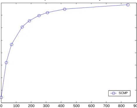
Figure 1 depicts the welfare losses associated with various degrees of mone-tary conservatismαfor the baseline calibration in section 5. For large values of
αthe welfare losses disappear and the steady state with SCMP approaches the
Ramsey steady state. Forα→ ∞ the conservative monetary reaction function
(MRF-C) becomes consistent with the Ramsey steady state, since the Lagrange
multiplier associated with MRF-C in problem (27) approaches zero.14 As a
result, for α → ∞ the fiscal authority’s policy problem (27) approaches the
Ramsey problem (16).15 In a setting with fiscal commitment, a sufficiently
conservative central bank thus eliminates the steady state distortions stemming from lack of monetary commitment.
7.2
Sequential Fiscal Policy
We now consider the case with sequential monetary andfiscal policy. Since the
monetary andfiscal authorities now pursue different objectives, it matters for
the equilibrium outcome whether fiscal policy is determined before, after, or
simultaneously with monetary policy. It remains to be ascertained, however,
1 4This holds only from a ‘steady state’ or ‘timeless’ perspective. Initially, the Lagrange
multiplier associated with MRF-C in (27) is non-zero.
which of these timing structures is the most relevant one for actual economies.
While it might take long to implement fiscal policies, the time lag between a
monetary policy decision and its effect on the economy can also be substantial.
We thus consider Nash as well as leadership equilibria.
7.2.1 Defining Nash and Leadership Equilibria
This section defines the various equilibria then briefly discusses them. For the case with simultaneous decisions we propose the following definition.
Definition 7 (SCMFP-Nash) A Markov-perfect equilibrium with sequential and conservative monetary policy, sequentialfiscal policy and simultaneous pol-icy decisions is a sequence{ct, ht,Πt, Rt, gt}∞t=0solving (11), (12), (15), (FRF),
and (MRF-C).
Next, consider the case with monetary leadership. The conservative mone-tary authority then has to take into account thefiscal reaction function (FRF).
The monetary authority’s policy problem at timet is thus given by:
max {ct+j,ht+j,Πt+j,Rt+j,gt+j} Et ∞ X j=0 βj³u(ct+j, ht+j, gt+j)− α 2(Πt+j−1) 2´ (28) s.t.:
Equations (11),(12),(15),(FRF) for allt
Et(ct+j, ht+j,Πt+j, gt+j, Rt+j) given forj≥1 Rt+j≥1for allj≥0
Eliminating Lagrange multipliers from thefirst order conditions of problem (28) delivers the conservative monetary reaction function with monetary leadership that we denote by (MRF-C-ML).
Definition 8 (SCMFP-ML) A Markov-perfect equilibrium with sequential and conservative monetary policy, sequential fiscal policy and monetary policy de-ciding beforefiscal policy is a sequence{ct, ht,Πt, Rt, gt}∞
t=0 solving (11), (12),
(15), (FRF), and (MRF-C-ML).
Finally, we consider the case withfiscal leadership. Fiscal policy must then take into account the conservative monetary reaction function(MRF-C):
max {ct+j,ht+j,Πt+j,Rt+j,gt+j} Et ∞ X j=0 βju(ct+j, ht+j, gt+j) (29) s.t.
Equations (11),(12),(15), (MRF-C) for allt
Et(ct+j, ht+j,Πt+j, gt+j, Rt+j) given forj≥1 Rt+j≥1for allj≥0
Solving for thefirst order conditions of problem (29) and eliminating Lagrange multipliers delivers thefiscal reaction function in the presence of a conservative
monetary authority andfiscal leadership that we denote by (FRF-C-FL).
Definition 9 (SCMFP-FL) A Markov-perfect equilibrium with sequential and conservative monetary policy, sequentialfiscal policy, and fiscal policy deciding before monetary policy is a sequence {ct, ht,Πt, Rt, gt}∞
t=0 solving (11), (12),
(15), (FRF-C-FL), and (MRF-C).
As before, the steady states corresponding to the equilibrium definitions 7, 8, and 9 are defined as the stationary values(c, h,Π, R, g)solving the equations listed in the respective definitions.
We now briefly comment on the previous definitions. First, note that for
the case α = 0 all three equilibria reduce to the one emerging under SMFP
without conservatism: MRF-C and MRF-C-ML are then identical to MRF and FRF-C-FL is identical to FRF. Second, for the Nash and monetary leadership cases, there exists a theoretical upper bound on the welfare gains that mone-tary conservatism is able to generate. Since in these cases the fiscal authority takes monetary decisions as given, welfare maximizing monetary behavior is the one consistent with the self-confirming equilibrium with sequentialfiscal policy (SFP) considered in section 4.2.1. Third, in the case withfiscal leadership, the fiscal authority anticipates the monetary reaction function and conservatism can then lead outcomes that are welfare superior outcomes to the one emerging with SFP.
7.2.2 The Implications of Central Bank Conservatism
Figure 2 displays the welfare gains associated with different degrees of monetary conservatism under the various leadership assumptions for the baseline
calibra-tion in seccalibra-tion 5. The upper and lower horizontal lines shown in the figure
indicate the welfare losses associated with SFP and SMFP, respectively.
For α= 0, i.e., the case without any monetary conservatism, all equilibria
deliver the welfare losses associated with SMFP. This is just a restatement of the fact that the leadership structure does not matter when both policymakers pursue the same objectives.
With SCMFP-Nash and SCMFP-ML wefind that an appropriately
conser-vative central bank can fully recover the steady state associated with monetary
commitment and sequential fiscal policy (SFP). The Nash and the monetary
leadership equilibria thus suggest that the gains from monetary conservatism can be substantial and that one can fully recover the welfare losses resulting from lack of monetary commitment with an appropriate degree of monetary conservatism. Interestingly, the costs associated with being overly conservative
appear small, while an insufficient degree of conservatism may result in large
The case for a conservative monetary authority is even stronger with
SCMFP-FL. As shown in figure 2, a conservative monetary authority then not only
eliminates the welfare losses from sequential monetary decisions but also those
emerging from lack offiscal commitment. In the limiting case ofα→ ∞
mone-tary conservatism fully recovers the Ramsey steady state.
Fiscal leadership differs from the Nash and monetary leadership cases
be-cause thefiscal authority anticipates the within-period off-equilibrium behavior
of the conservative monetary authority. Forα→ ∞the monetary authority is
determined to implement price stability at all costs. A fiscal expansion above
the Ramsey spending level, which generates inflation, then triggers a strong
increase in interest rates so as to reduce private consumption. Thus, in this setting thefiscal authority anticipates thatfiscal spending results in a crowding out of private consumption and this disciplines thefiscal authority’s behavior.
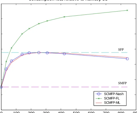
Figure 3 displays the steady state values associated with various degrees of
monetary conservatism for the different timing assumptions. While monetary
conservatism unambiguously reduces the inflation bias, its effect on the fiscal
spending bias depends on whether or notfiscal policy anticipates the monetary
policy decision. Iffiscal policy takes the monetary decision as given, monetary conservatism results in an increasedfiscal spending bias for the reasons discussed in section 4.2.1. This explains why in the Nash and monetary leadership cases
an overly conservative central bank reduces welfare, see figure 2. The gains
from lowering inflation at some point start to be outweighed by the losses from increasedfiscal spending and the resulting crowding out of private consumption. Figure 3 also explains why insufficient monetary conservatism is rather costly in welfare terms, while an overly conservative central bank does not cause much welfare losses in the Nash and monetary leadership cases. With too much mon-etary conservatism, the public spending increase and the resulting crowding out
of private consumption roughly offset each other in utility terms. At the same
time, there are large initial welfare gains from monetary conservatism, which arise from correcting the monetary inflation bias. Unlike in the case with exoge-nousfiscal policy, however, the inflation bias has to be defined as the inflation increase associated with a transition from the SFP regime to the SMFP regime.
8
Conclusions
This paper analyzes monetary andfiscal policy interactions in a dynamic general equilibrium model when policymakers lack the ability to credibly commit to policies ex-ante.
It is shown that lack offiscal commitment leads to excessivefiscal spending on public goods while lack of monetary commitment results in the well-known inflation bias. The welfare losses generated by lack of monetary or fiscal com-mitment appear to be substantial. In the absence of monetary comcom-mitment,
independently of whether or notfiscal policy can commit, making the monetary authority appropriately conservative completely eliminates the steady state dis-tortions associated with sequential monetary policy. The case for a conservative monetary authority is even stronger because monetary conservatism may also eliminate the steady state losses associated with lack offiscal commitment.
A number of important questions remain to be addressed in further research. First, the paper considers steady state effects only. In a fully stochastic model, however, welfare losses also depend on the conditional response to shocks.
Ex-ploring the effects of monetary conservatism on these policy responses seems
to be of interest. Second, the paper abstracts from capital stock and govern-ment bond dynamics, which would allow for additional interactions between policymakers. We plan to extend the analysis to such richer settings in future work.
A
Appendix
A.1
Proof of Lemma 1
Suppose the steady state inflation rate is given byΠ∈[β, β−1]. Forβsufficiently close to 1, the sign of the l.h.s. of MRF is determined by the sign of
µ 1 + uc uh ¶ 2Π−1 Π−1 = (1−w(1−τ))2Π−1 Π−1 (30)
Monopolistic competition impliesw <1. Sinceτ≥0, it follows that 1−w(1−
τ)6= 0, which shows that MRF cannot be satisfied for a steady state inflations rateΠ ∈[β, β−1], provided β is sufficiently close to one. The Euler equation
(12) and the constraintR≥1imply thatΠ≥β in any steady state. Thus, it
must be thatΠ> β−1>1, as claimed.
A.2
Utility Parameters and Ramsey Steady State
Here we show how the utility parameters ω0 and ω1 are determined by the
Ramsey steady state values. Let variables without subscripts denote their steady
state values and consider a steady state whereΠ= 1. The Phillips curve (11)
then implies 1 +η− ω0η (1−h)c−σ − g+x h η= 0 (31) which delivers ω0= (1−h)¡1 +η−g+hxη¢ ηcσ (32)
Letγt1, γt2, γt3 be the Lagrange multipliers associated with (11), (12), and (15),
respectively, in problem (16). The first order condition (FOC) of (16) with
respect toRt implies
γ2= 0 (33)
The FOC with respect tocttogether with equations (31) and (33) deliver
c−σ+γ1 hω0ησ
(1−h)c−γ
3= 0 (34)
The FOC with respect tohtand equation (31) imply
− ω0 1−h+γ 1 Ã hω0η (1−h)2 − g+x h ηc −σ ! +γ3= 0 (35)
Equations(34)and(35)determine
γ1= ω0 1−h−c−σ hω0η (1−h)2 + hω0ησ (1−h)c− g+x h ηc−σ (36) γ3=c−σ+γ1 hω0ησ (1−h)c (37)
From the FOC with respect togtit then follows that
ω1=g(γ3−γ1c−ση) (38) Given steady state values forc, h, gandxconsistent with the resource constraint (15), equations (32), and (36)-(38) determineω0 andω1.
References
Alesina, Alberto and Guido Tabellini, “Rules and Discretion with
Non-coordinated Monetary and Fiscal Policies,” Economic Inquiry, 1987, 25,
619—630.
Barro, Robert and David B. Gordon, “A Positive Theory of Monetary
Policy in a Natural Rate Model,” Journal of Political Economy, 1983,91,
589—610.
Chari, V. V. and Patrick J. Kehoe, “Sustainable Plans,”Journal of Polit-ical Economy, 1990,98, 783—802.
and , “Optimal Fiscal and Monetary Policy,” in John Taylor
and Michael Woodford, eds., Handbook of Macroeconomics, Amsterdam:
Díaz-Giménez, Javier, Giorgia Giovannetti, Ramon Marimon, and Pedro Teles, “Nominal Debt as a Burden on Monetary Policy,”Pompeu Fabra University Mimeo, 2004.
Dixit, Avinash and Luisa Lambertini, “Monetary-Fiscal Policy
Interac-tion and Commiment Versus DiscreInterac-tion in a Monetary Union,” European
Economic Review, 2001, 45, 977—987.
and , “Interactions of Commitment and Discretion in Monetary and
Fiscal Policies,”American Economic Review, 2003,93, 1522—1542.
and , “Symbiosis of Monetary and Fiscal Policies in a Monetary
Union,”Journal of International Economics, 2003,60, 235—247.
Fudenberg, Drew and David Levine, “Sef-Confirming Equilibrium,”
Econometrica, 1993,61, 523—545.
Klein, Per Krusell Paul and José-Víctor Ríos-Rull, “Time Consistent
Public Expenditure,”CEPR Discussion Paper No. 4582, 2004.
Kydland, Finn E. and Edward C. Prescott, “Rules Rather Than
Discre-tion: The Inconsistency of Optimal Plans,”Journal of Political Economy,
1977,85, 473—492.
Leeper, Eric M., “Equilibria under Active and Passive Monetary and Fiscal
Policies,”Journal of Monetary Economics, 1991,27, 129—147.
Lucas, Robert E. and Nancy L. Stokey, “Optimal Fiscal and Monetary
Policy in an Economy Without Capital,”Journal of Monetary Economics,
1983,12, 55—93.
Ramsey, Frank P., “A Contribution to the Theory of Taxation,” Economic Journal, 1927,37, 47—61.
Rogoff, Kenneth, “The Optimal Degree of Commitment to and Intermediate
Monetary Target,”Quarterly Journal of Economics, 1985,100(4), 1169—89.
Rotemberg, Julio J., “Sticky Prices in the United States,”Journal of Political Economy, 1982,90, 1187—1211.
Sargent, Thomas J.,The Conquest of American Inflation, Princeton: Prince-ton Univ. Press, 1999.
and Neil Wallace, “Some Unpleasant Monetarist Arithmetic,” Federal Reserve Bank of Minneapolis Quarterly Review, 1981,5(3).
Sbordone, Argia, “Prices and Unit Labor Costs: A New Test of Price
Sticki-ness,”Journal of Monetary Economics, 2002,49, 265—292.
Schmitt-Grohé, Stephanie and Martín Uribe, “Optimal Fiscal and
Mon-etary Policy under Sticky Prices,” Journal of Economic Theory, 2004,
and Martin Uribe, “Optimal Simple and Implementable Monetary and
Fiscal Rules,”Duke University mimeo, 2004.
Svensson, Lars E. O., “Optimal Inflation Targets, ’Conservative’ Central
Banks, and Linear Inflation Contracts,”American Economic Review, 1997,
87, 98—114.
Walsh, Carl E., “Optimal Contracts for Central Bankers,” American Eco-nomic Review, 1995, 85, 150—67.
Woodford, Michael, “Doing Without Money: Controlling Inflation in a
Post-Monetary World,”Review of Economic Dynamics, 1998,1, 173—209.
, “Public Debt and the Price Level,”Princeton University mimeo, 1998.
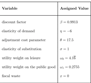
Variable Assigned Value
discount factor β= 0.9913
elasticity of demand η=−6
adjustment cost parameter θ= 17.5
elasticity of substitution σ= 1
utility weight on leisure ω0= 4.16
utility weight on the public good ω1= 0.2755
fiscal waste x= 0
Table 1: Baseline calibration
Policy c h g Π τ Welfare equivalent
regime (percentage deviations relative to Ramsey) (level) consumption losses
SFP -16.6% 0.7% 55.0% 2.6% 36.8% -6.5%
SMP 5.9% 10.5% -16.9% 4.6% 17.9% -7.6%
SMFP -6.6% 14.8% 29.6% 5.7% 26.9% -11.0%
Welfare equivalent
consumption losses ΠSM F P−ΠSF P
SFP SMP SMFP
Baseline calibration -6.5% -7.6% -11.0% 3.1%
more sticky prices (θ= 25) -6.8% -8.2% -11.9% 2.8%
less sticky prices (θ= 10) -5.8% -6.6% -9.5% 3.5%
almostflexible prices (θ= 0.1) -0.5% -0.5% -0.6% 2.0%
more competition (η=−7) -4.6% -6.2% -8.7% 2.9%
less competition (η=−5) -9.8% -9.4% -14.2% 2.8%
fiscal waste (x= 0.02) -3.0% -7.8% -9.5% 4.3%
higher risk aversion (σ= 2) -1.2% -3.3% -4.2% 2.9%
lower risk aversion (σ= 0.4) -37.2% -19.8% -37.2% 0.0%
very low risk aversion (σ= 0.35) -43.8% -22.4% -45.4% -0.6%
0 100 200 300 400 500 600 700 800 900 -8 -7 -6 -5 -4 -3 -2 -1 0
Consum ption loss re la tive to Ra mse y SS
Degree of conservatism (alpha)
P e rc en tage poi nt s SCMP
0 100 200 300 400 500 600 700 800 900 -14 -12 -10 -8 -6 -4 -2 0
Consumption loss relative to Ramsey SS
Degree of conservatism (alpha)
P e rc e n tage po in ts SCMFP-Nash SCMFP-FL SCMFP-ML SFP SMFP
0 100 200 300 400 500 600 700 800 900 1 1.01 1.02 1.03 1.04 1.05 1.06 1.07 Inflation alpha SCMFP-Nash SCMFP-FL SCMFP-ML 0 100 200 300 400 500 600 700 800 900 0.045 0.05 0.055 0.06 0.065 0.07 Government spending alpha SCMFP-Nash SCMFP-FL SCMFP-ML 0 100 200 300 400 500 600 700 800 900 0.125 0.13 0.135 0.14 0.145 0.15 0.155 Private consumption alpha SCMFP-Nash SCMFP-FL SCMFP-ML 0 100 200 300 400 500 600 700 800 900 0.19 0.195 0.2 0.205 0.21 0.215 0.22 0.225 0.23 0.235 Working hours alpha SCMFP-Nash SCMFP-FL SCMFP-ML