Hypersonic Chemically Reacting Boundary-Layer Stability
using LASTRAC
H.L. Kline∗
National Institute of Aerospace, Hampton, VA, 23666 C.-L. Chang†and F. Li‡
NASA Langley Research Center, Hampton, VA, 23681
Hypersonic boundary layer transition is critical to the design of all hypersonic vehicles due to its effect on the heat transfer into the vehicle surface and potential drag enhancement or re-duction during reentry. Boundary layer transition and boundary layer stability analysis under hypersonic conditions has been studied for decades, yet there is ample room for improved accuracy and further investigations into the relevant phenomena. In this work, we present a recent implementation of chemical equilibrium, finite-rate chemistry, and thermochemical nonequilibrium capabilities into LASTRAC, an existing well-established boundary-layer stabil-ity analysis code. Verification against existing numerical results in the literature are presented. LASTRAC was previously able to address calorically perfect flows. By using solutions of the Parabolized Stability Equations (PSE) with chemical and thermal nonequilibrium, we are able to investigate the effects of chemical and thermal nonequilibrium on a variety of phenomena including stationary crossflow instability on a swept wing and 2nd mode instabilities over a
wedge.
I. Nomenclature
ρ = density [kg m−3]
p = pressure [Pa]
T = temperature [K]
h = enthalpy per unit mass [J kg−1]
e = energy per unit mass [J kg−1
]
Cs = mass fraction for species s
k = thermal conductivity [J m−1s−1K−1] t = time [s] f = frequency [Hz] ` = length scale [m] x,y,z = body-fitted coordinates h1,h3 = curvature terms ~ V ={u,v,w} = velocity vector [m/s] Ms = molar mass for species s [g] ms = particle mass for species s [g]
γ = ratio of specific heats
γs = molar concentration for species s
µ = kinematic viscosity [N s m−2]
ν = dynamic viscosity [kg s−1m−1]
λ = 2nd viscous coefficient [N s m−2 ]
αs,r,βs,r = stoichiometric coefficients
Rf,r,Rb,r = forward and backward reaction rates
τs = vibrational-translational relaxation time [s]
∗
Research Engineer, Research Department, MS 128, AIAA Member.
†
Aerospace Technologist, Computational Aerosciences Branch, MS 128, Associate Fellow, AIAA.
‡
Aerospace Technologist, Computational Aerosciences Branch, MS 128.
˙
ωs = species production rate [kg m−3s−1]
Dsr = diffusion coefficient of species s with respect to species r [m2s−1] Ds = diffusion coefficient of species s with respect to the mixture [m2s−1] Cp,Cv = constant pressure and volume specific heats [J mol−1K−1]
Cp,s,Cv,s = constant pressure and volume specific heats for species s [J mol−1K−1] Cv,Vs = constant volume specific heat for vibrational energy for species s [J mol−1K−1]
S = entropy [J mol−1
K−1]
πΩ¯(1,1)
i j ,πΩ¯
(2,2)
i j = collision integrals between species i and j [m2] ∆(1)
i j,∆
(2)
i j = modified collision integrals between species i and j [m s]
kB = Boltzmann’s constant [J K−1]
Av = Avogadro’s number [mol−1
Ru = universal gas constant [J mol−1K−1]
Re = Reynolds number Le = Lewis number Pr = Prandtl number Ec = Eckert number M = Mach number F = nondimensionalized frequency φ = disturbance vector ()s = species quantity
()e = edge of boundary layer
()d = dimensional quantity ¯ () = mean value ()0 = disturbance value ()el = electronic value ()V = vibrational-electronic value ()t r = translational-rotational value
II. Introduction
H
ypersonic boundary layer transition is critically important to hypersonic vehicle design due to its influence on heattransfer rates, and has been the subject of previous research [1–3]. Under hypersonic conditions the temperature within the boundary layer may rise to a point where chemical reactions occur, and depending on the circumstances, this may include chemical equilibrium, finite-rate chemical nonequilibrium where the gas composition is actively changing and does not reach chemical equilibrium, or thermochemical nonequilibrium where the relaxation time of translational and vibrational temperatures is such that separate relaxation temperatures should be tracked.Saric et al. [4] reviewed the instability mechanisms that lead to laminar-turbulent transition, which can be categorized as streamwise (Mack 1st and 2ndmodes), crossflow, supersonic, centrifugal (Görtler), and attachment-line. In this work, we examine 2ndmode, supersonic mode, and stationary crossflow instabilities. Crossflow instabilities are of particular interest because current methods for delaying transition due to crossflow instabilities are limited to minimizing the extent of crossflow occurring in the boundary layer, and so further investigation into what parameters affect crossflow instabilities under hypersonic conditions is of interest. Predicting the exact point of transition is a difficult task that requires not only detailed analysis of boundary layers stability, but also detailed knowledge of the disturbances that will be encountered. Under most situations, the exact point of transition cannot be predicted due to a lack of knowledge about the disturbance environment. The accepted practice is to reduce the N-factor of a vehicle design in order to delay transition and improve the performance through a reduction of the percentage of the surface impacted by turbulent flow, despite not knowing the exact point of transition.
Kimmel [5] provides a thorough review of hypersonic transition control techniques, and states that one of the difficulties of hypersonic transition control is that the techniques applied at lower speeds cannot be extrapolated to the high heating environment and the physical phenomena occurring within these boundary layers. At the same time, the potential benefits of a greater understanding of hypersonic boundary layer transition are significant. Analysis of the National AeroSpace Plane (NASP) aerodynamics [6] estimated that the possible payload of an air-breathing single-stage-to-orbit vehicle would double if it was fully laminar as compared to fully turbulent. Techniques to control
transition include wall cooling, which is effective in stabilizing the first Mack mode but destabilizing to the 2nd mode [5, 7]. The second mode is usually held to be more dominant, however, this may change due to the magnitude and frequency of freestream noise as well as the vehicle geometry, where some differences have been seen when comparing planar to conical geometries [8]. In some cases, cooling is necessary to prevent material failure, even when the more dominant second mode will be destabilized. A better understanding of the effects of cooling on transition will help determine when the decreased performance due to increased turbulence will outweigh the prevention of melting and increased material flexibility as the structure temperature increases. Determining whether the inclusion of chemical kinetic and thermochemical effects changes this prediction can help to decide on the minimum simulation fidelity required for initial studies: if the effect of wall cooling is significantly different with chemical kinetic or thermochemical effects are included, then it would be advantageous to include such effects during design studies that modify the wall cooling rate. While wall-temperature calculations have been conducted before, such as by Malik [9], chemistry is tightly linked to temperature and so the inclusion of a chemistry model is interesting to examine.
To the authors’ knowledge, STABL-3D or PSE-Chem is the only available tool to address thermochemical nonequilibrium boundary layer stability [1, 10–12] with PSE. By contrast, the Langley Stability and Transition Analysis Code (LASTRAC), although previously limited to calorically perfect gases, includes nonlinear PSE capabilities and other tools such as adjoint-PSE based receptivity modules. LASTRAC is an existing well-established boundary-layer stability analysis code [13]. The work presented here is an initial step toward implementing nonequilibrium effects in LASTRAC, with future work planned to add thermochemical and chemical nonequilibrium capabilities for nonlinear and linear PSE as well as general 3D boundary layers. Comparison between LASTRAC and PSE-Chem should allow confirmation of both and aid further development. Boundary layer stability with thermochemical nonequilibrium has also been investigated by Bertolotti [14] and Wang [15] using Linear Stability Theory and by Zhong [16] as well as by Knisely and Zhong [17] through the use of Direct Numerical Simulation. Parabolized Stability Equation analysis under conditions of thermal equilibrium was investigated by Chang et al. [3], Miró et al. [18], and Malik [2]. The long term goal for LASTRAC development is to provide a general transition prediction tool set for all speed regimes, from low-speed to hypersonic.
III. Methodology
Boundary layer stability analysis will be described with discussion of what changes when chemical effects are added, followed by the boundary conditions used for stability analysis, the chemical and thermodynamic models used, as well as the techniques used to produce the mean flow solutions.
A. Boundary Layer Stability Analysis
LASTRAC includes capabilities to analyze boundary layer stability with quasiparallel Linear Stability Theory (LST) and Parabolized Stability Equations (PSE). The LST method assumes that the boundary layer is nearly parallel, with negligible growth of the thickness of the boundary layer, while PSE takes into account the variation of the boundary layer thickness and changing shape of the disturbance field in the streamwise direction. While an eigenvalue problem is formed in both the LST and PSE approaches, the PSE method numerically solves an approximate form of the governing partial differential equations for the slow-varying shape function with an actively updated wave number along the streamwise direction, using the eigenvalue solution as the initial value. The Nonlinear PSE retains nonlinear terms from the Navier-Stokes equations, and requires a known finite disturbance. Both LST and linear PSE are independent of the input disturbance amplitude but only valid for sufficiently small disturbances. In the current work, the Langley Stability and Transition Analysis Code (LASTRAC) was modified in this work to include chemically reacting flows and thermal nonequilibrium. Further detail on the capabilities previously available in LASTRAC is described in the LASTRAC manual [13]. The methodology will be summarized here, with particular attention to the points that were modified to accommodate gas chemistry effects.
Stability equations are derived starting from the nondimensionalized Navier-Stokes equations, ∂ ρ ∂t +∇ · ρV~ =0 ρ ∂V~ ∂t + ~ V · ∇V~ =−∇p+ 1 Re ∇[λ(∇ ·V~)]+∇ ·[µ(∇V~ +∇V~T)] ρCp "∂ T ∂t +( ~ V· ∇)T # = 1 RePr∇ ·(k∇T)+Ec ∂p ∂t +( ~ V· ∇)p ! +EcΦ Re. (1)
For a calorically perfect gas,
Φ=λ(∇ ·V~)2+ µ 2 f ∇V~+∇V~Tg2 µ= f(T), λ=2 3 (s−1)µ p=ρRT, Cp =const, R=const, (2)
wheresis the Stokes parameter,µis the viscosity,λis the second coefficient of viscosity,Ris the gas constant,Cp
is the specific heat at constant pressure,pis the pressure, ρis the density,V~ ={u,v,w}is the velocity, andT is the temperature. Nondimensional numbers that appear in the equations are: the Reynolds number, Lewis number, Prandtl number, Eckert number, and Mach number:
Re=ue` νe Le= ρeDeCp,e ke Pr = µeCp,e ke Ec= u2e Cp,eTe =(γe−1)M 2 e, Me= | ~ Ve| √ γeReTe, (3)
where all normalizing values are taken at the edge of the boundary layer. Equation Set 1 has been nondimensionalized with: T =Td/Te ρ=ρd/ρe V~ =V~d/ue p=pd/(ρeu2e) `= √ νexd/ue µ=µd/µe x=xd/` k=kd/ke Cp=Cp,d/Cp,e, (4)
where the subscript eindicates the dimensional value at the edge of the boundary layer along the normal to the surface, and the subscriptdindicates the local dimensional quantity. The quantity`is the dimensional boundary layer length scale, andxdis the dimensional coordinate in the streamwise direction. Quantities that have no subscript are nondimensional unless otherwise stated. We take the solution to be composed of the mean flow and a fluctuation,
u=u¯+u0 v= ¯ v+v0 w= ¯ w+w0 p=p¯+p0 ρ=ρ¯+ρ0 T =T¯+T0 µ=µ¯+µ0 λ=λ¯+λ0 k=k¯+k0, (5)
which is substituted into Equation Set 1. A body-fitted orthogonal coordinate system will be used wherex,y, andzare defined as streamwise, wall-normal, and spanwise, respectively. Element lengths areh1dx,dy, andh3dz, accounting for streamwise and transverse curvature in thexandzdirections. Subtracting Equation Set 1 for the mean flow and stating the result in terms of Jacobians and the disturbance vectorφ={p0,u0,v0,w0,T0}T,
Γ∂φ ∂t + A h1 ∂φ ∂x +B ∂φ ∂y + C h3 ∂φ ∂z +Dφ= 1 Re0 * , Vx x h2 1 ∂2φ ∂x2 + Vx y h1 ∂2φ ∂x∂y+Vy y ∂2φ ∂y2 +Vx z h3 ∂2φ ∂x∂z+ Vy z h3 ∂2φ ∂y∂x+ Vz z h2 3 ∂2φ ∂z2 + -, (6)
whereΓ,A,B,C,D,Vx x,Vx y,Vx z,Vy z, andVz zare the Jacobians for this system. Re0 =
ue`0
νe , where`0is the reference
Since the Jacobians at this point depend on perturbed quantities, there are second- and higher-order perturbations included in Equation 6. The linearized form is found by separating each Jacobian into two parts that respectively contain only mean flow quantities or only perturbation quantities, e.g.,A=A¯+A0. Becauseφis a vector of perturbed quantities, the linearized form of these equations retains only the mean flow portion of the Jacobians,
¯ Γ∂φ ∂t + ¯ A h1 ∂φ ∂x +B¯ ∂φ ∂y + ¯ C h3 ∂φ ∂z +D¯φ= 1 Re0 * , ¯ Vx x h2 1 ∂2φ ∂x2 + ¯ Vx y h1 ∂2φ ∂x∂y+V¯y y ∂2φ ∂y2 +V¯x z h3 ∂2φ ∂x∂z+ ¯ Vy z h3 ∂2φ ∂y∂x+ ¯ Vz z h2 3 ∂2φ ∂z2 + -. (7)
The disturbance fieldφis assumed to be periodic in space and time, and so the disturbance vector can be expressed as a Fourier series, φ(x,y,z,t)= M X m=−M N X n=−N χmn(x,y)ei(nβz−mωt), (8)
whereM andNrepresent the numerical resolution in time and space, respectively. The fundamental temporal wave number is a nondimensionalized form of the physical frequency f,ω=2uπ`e f.
Substituting a single disturbance mode defined by the wave numberω= 2uπ`e f and spanwise wave numberβ=
2π
λz
in Equation 7 results in the Linearized Navier-Stokes (LNS) equation,
¯ A h1 − iβV¯x z h3Re0 !∂ χ ∂x + B¯+ iβV¯y z h3Re0 !∂ χ ∂y +* , ¯ D−iωΓ¯+iβC¯ h3 + β2V¯ z z h2 3Re0 + -χ= 1 Re0 * , ¯ Vx x h2 1 ∂2χ ∂x2 + ¯ Vx y h1 ∂2χ ∂x∂y+V¯y y ∂2χ ∂y2+ -. (9)
This equation can be solved numerically, and simplifications lead to approximate solutions that are obtained at a lower computational cost for engineering applications. One such simplification is the quasiparallel assumption that neglects the velocity normal to the wall and all mean flow variation in thexdirection. The linear Parabolized Stability Equations (PSE) decompose the mode shape into two parts: a complex wave numberαthat varies only inxand a shape function that varies inxandy,
χ= χˆ(x,y)ei Rx
x0α(ξ)dξ,
(10) where ξis the variable of integration. The resulting equations are solved as a set of parabolized equations, which allows for an efficient marching solution that consists of shape functions, producing solutions for the shape function variations and disturbance growth rate as a function of the imaginary part ofα. The quasiparallel assumption leads to the Linear Stability Theory (LST) eigenvalue solutions, where the shape function is a function ofyonly. Further details are available in the LASTRAC manual [13].
Equation Set 1 applies to a calorically perfect gas. In this work, four gas models are included: a calorically perfect gas, a mixture of thermally perfect gases in chemical equilibrium, a mixture of thermally perfect gases using a finite-rate chemical kinetic model, and thermochemical nonequilibrium. In order to address these models, the equations are rederived to include updated relationships for transport and thermodynamic properties. The resulting equations remain in the same form shown in Equation 9, with the contents and dimensions ofφ, χ, and the Jacobian matrices updated.
For a chemical equilibrium mixture of thermally perfect gases, the dimension of the problem remains the same; but the relationships for transport properties as well as the state equation must be updated and this changes terms within the Jacobians. Gibbs free energy minimization is used to produce the chemical equilibrium gas state for a given thermodynamic state defined by two state variables. Quantities such as density (ρ), viscosity (µ), and specific heat (Cp) change, as well as their gradients with respect to pressure (p), velocity (u,v,w), and temperature (T). In the state equation,Ris no longer a constant, and depends on the equilibrium gas composition.
For finite-rate chemistry, additional equations are necessary to calculate the species mass fractions and their disturbances. The continuity and momentum equations remain unchanged, using mixture values for ρ, p, and µ. Equations governing species production and destruction are added, and the energy equation must be updated to include
energy changes from the chemical reactions. Drawing from MacCormack and Candler [19], Chang et al. [3] and Anderson [20], and nondimensionalizing,
ρ ∂Cs ∂t +∇ · CsV~ ! = Le RePr∇ ·(ρDs∇Cs)+ω˙s, s=1. . .Ns ρCp "∂ T ∂t +( ~ V· ∇)T # = 1 RePr∇ ·(k∇T)+Ec ∂p ∂t +( ~ V · ∇)p ! +EcΦ Re + Le RePr Ns X s=1 ∇(hs)·(ρDs∇Cs) + Ns X s=1 hsω˙s, (11) where: Cp = Ns X s=1 CsCp,s ρ= Ns X s=1 ρs= p RuPCMssT Cs =ρs/ρ , X Cs =1 ˙ ωs,d =Ms Nr X r=1 βs,r−αs,rR f,r −Rb,r ˙ ωs =ω˙s,dρ` eue . (12)
Msis the species molecular mass,Ru the universal gas constant,ρsis the species density,Nsis the number of species in the gas mixture, ˙ωs represents the nondimensionalized species production rate due to chemical reactions,Ds is the diffusivity of speciesswith respect to the gas mixture normalized by the value at the boundary-layer edgeDe, andhs is the enthalpy per unit mass of speciessnondimensionalized by edge temperature and heat capacity. The terms βs,randαs,r are the stoichiometric coefficients for theNrreactions being considered, andRf,randRb,rare the associated reaction rates. Equation Set 11 is nondimensionalized in a manner similar to Equation Set 1. The mean flow disturbance vector now includes species mass fractions,Cs =C¯s+Cs0, in addition to the disturbances listed in
Equation 5. The governing equation for the disturbances including species mass fractions can be expressed in the same form as Equation 6, with the difference that the Jacobians are now of a larger dimension and contain terms from the species mass fraction equations and new terms in the energy equation that depend on the mass fractions.
In the previous equations, thermal equilibrium was assumed. This means that the vibrational, electron, translational, and rotational energies had equilibrated and a single temperature is sufficient. In other words, we assume that the relaxation time between these energy modes is sufficiently shorter than the time scale of the flow phenomena. This is not necessarily true for hypersonic problems. For thermal nonequilibrium, multiple temperatures are required. In this work, we will use a two-temperature model for thermochemical equilibrium, where the vibrational-electronic energies are associated withTV =Tvib =Tel ec, and the translational-rotational energy is associated withT =Tt r an s =Tr ot. As compared to thermal equilibrium with chemical nonequilibrium (the finite-rate chemistry model), an additional equation and variable are added to the system, with the associated disturbanceTV0. In addition, the chemistry model will take into account different rate controlling temperatures based onTandTVdepending on what type of reaction is occurring. The total energy equation is updated,
ρCp "∂ T ∂t +( ~ V· ∇)T # +ρCp,V "∂ TV ∂t +( ~ V· ∇)TV # = 1 RePr∇ ·(k∇T+kv∇TV)+Ec ∂p ∂t +( ~ V · ∇)p ! +EcΦ Re + Le RePr Ns X s=1 ∇(hs)·(ρDs∇Cs) + Ns X s=1 hsω˙s, (13)
and a vibrational-electronic energy equation is added: ρCp,V "∂ TV ∂t +( ~ V· ∇)TV # = 1 RePr∇ ·(kv∇TV)+Ec ∂pel ∂t +( ~ V· ∇)pel ! + Le RePr Ns X s=1 ∇(hv,s)·(ρDs∇Cs) + X s=mol ρs (e∗v,s−ev,s) < τs > +2 ρel3 2 ¯ R(T−TV) Ns−1 X s=1 νe s Ms − X s=io n s ˙ ne,sIˆs+ Ns X s=1 ˙ ωsDˆs, (14)
where theTV is normalized by the boundary layer edge value of the translational temperatureTe,Cp,Vis the constant pressure specific heat for electron-vibrational energy modes andCp,VTV =ev, the combined electron and vibrational energy.Cp,Vis normalized by the edge specific heatCp,e, and the remaining terms are similarly nondimensionalized. The vibrational thermal conductivitykv, vibrational-translational relaxation time< τs >, species vibrational enthalpy hv,s, vibrational energy per unit mass of diatomic molecules ˆDshave been added, and are provided by the chemistry model. In this work, electron and ion species are not included, and so ionization and electron related terms such as the electron pressurepel, collision frequency between electrons and neutral particlesνe s, rate of ion production ˙ne,sand ionization energy ˆIswill not be needed. Terms dependent on the chemistry model are discussed further in Section C, and terms specific to thermochemical nonequilibrium in Equations 30–34.
The included results are presented in terms of a nondimensional frequencyF, the complex part of the wavenumber
αi, and the N-factor based on disturbance kinetic energy,
F =2π` ue f αi ==(α(x)) E= Z ye 0 ρ(|u0|2+|v0|2+|w0|2)dy σ(x)=−αi(x)+ 1 2E dE dx N(x)= Z x x0 σ(ξ)dξ . (15)
The N-factorNrefers to the integrated growth rate,σ, based on disturbance kinetic energyE, which is evaluated to the edge of the boundary layerye. The integral definingNis evaluated with the neutral point where the imaginary growth rate first becomes negative as the lower bound. The critical N-factor (Ncr i t) is the value of the N-factor where transition would be expected to occur based on experimental correlations. Whenαi is negative the associated eigenmode is unstable.
B. Boundary Conditions
The boundary conditions of the PSE problem are determined by the linearization of the boundary conditions of the mean flow problem. As discussed in the LASTRAC manual [13], for a no-slip boundary condition,
u=v=w=0 (u¯+u0)=(v¯+v0)=(w¯+w0)=0 u0=v0=w0=0.
(16)
Similarly, for an isothermal solid wall,
TV =T =Tw ¯ TV+TV0 =T¯+T 0=T w TV0 =T0=T¯+T0−Tw =0. (17)
We now add the boundary conditions for noncatalytic and fully-catalytic wall boundary conditions. At a noncatalytic wall, the gradient of the species mass fractions with respect to the wall normal direction is zero, ∂C∂yi =0 due to an
assumption of no chemical reactions occurring on the wall surface. For a partially catalytic wall, reactions are assumed to occur at a constant, prescribed, rate. As the noncatalytic and partially-catalytic conditions lead to the same boundary condition for the species perturbations, for either case:
∂Ci ∂y =const ∂(C¯i+Ci0) ∂y =const ∂Ci0 ∂y = ∂(C¯i+Ci0) ∂y − ∂Ci ∂y =0. (18)
For a fully catalytic wall, species mass fractions take the equilibrium value, Ci =Ci,e
Ci+Ci0=Ci,e
Ci0=0.
(19)
Therefore, at an isothermal, no-slip, noncatalytic wall:
u0=v0=w0=T0=TV0 = ∂C 0
i
∂y =0. (20)
No boundary condition is applied to the pressure or mixture density. The freestream boundary of the problem is defined at the edge of the boundary layer, and can be either a Dirichlet condition setting the perturbations to zero, or a nonreflecting boundary. A nonreflecting boundary is required when perturbations are expected to extend to or beyond the boundary layer edge, as is the case with supersonic modes. At the nonreflecting boundary the outgoing characteristic equations are used to set the disturbance boundary condition. Following [13],
Γ∂φ ∂t + A h1 ∂φ ∂x +B +∂φ ∂y + C h3 ∂z ∂z+Dφ=0, (21)
where B+ is formed using the positive eigenvalues and the left eigenvector matrix of the product of the coefficient matricesΓ−1Bgiven in Equation 7:
B+=Γ(LΛ+L−1) LΛL−1=Γ−1B
Λ=diag(λj)
Λ+=diag(max(0, λj)).
(22)
Viscous terms are assumed to be negligible, and as these equations are defined at the boundary layer edge, the gradients of~v,T, andρnormal to the boundary approach zero. The nonreflecting boundary conditions for equilibrium, finite-rate chemical nonequilibrium, and thermochemical nonequilibrium were implemented as part of this work, building on the existing boundary condition for a calorically perfect gas.
C. Chemical and Thermodynamic Models
A number of the quantities needed for boundary layer stability are dependent on the gas composition, including species production rates ˙ωs, transport properties viscosity and thermal conductivity, and thermodynamic quantities of specific heats and enthalpy. The chemistry model used in this work is similar to that developed by Thompson et al. [21] for the calculation of thermodynamic and transport properties, with modifications including the addition of thermochemical nonequilibrium terms, user-input collision integral curve fit coefficients, chemical reaction rate coefficients, and the use of the Chemical Equilibrium with Applications (CEA) format for thermodynamic curve fit coefficients, with the equations for specific heat, enthalpy, and entropy for each species from McBride et al. [22]:
Cp,s(T)/R=a1T−2+a 2T −1+a 3+a4T +a5T2+a6T3+a7T4 hs(T)/RT =−a1T −2+a 2lnT/T+a3+a4T/2+a5T2/3+a6T3/4+a7T4/5+b1/T Ss(T)/R=−a1T −2/ 2−a2T −1+ a3lnT+a4T+a5T2/2+a6T3/3+a7T4/4+b2, (23)
where the equations for enthalpy and entropy are found by integrating Cp,s andCp,s/T with respect to T. The Gibbs free energy can then be determined from the enthalpy and entropy for use in calculating the equilibrium state through minimization of the free energy. The constants for this curve fit are available from [23]. The finite-rate and thermochemical nonequilibrium models used reaction rate coefficients from Blottner [24] and Dunn & Kang [25] as combined by Gupta et al. [26]. For the 5-species model used in this work, only those reactions that contain O2, O, NO, N2, and N are considered.
In addition to the thermodynamic quantities, transport quantities of viscosity, thermal conductivity, and diffusion coefficients are required. These quantities are functions of collision integrals between all pairs of chemical species included in the model. The collision integrals or collision cross-sectionsπΩ¯(i,l,js)for momentum transfer are defined as
integrated functions of the differential cross section for the pair of species, the relative velocity and reduced velocities of the colliding particles, and the scattering angle. This equation can be found in Yos [27], and rather than evaluate the detailed expression for the collision cross-section at each temperature, curve fits based on cross-section values evaluated at a range of temperatures are commonly used in the literature [26, 28]. A curve fit for air is available from Gupta et al. [26]. According to collision integral data tabulated in by Wright [29], the uncertainty in the values of the collision integrals ranges anywhere from±5% to±50%, and so although a curve fit can match the data closely, it should not be expected to be any more accurate than the data used.
The curve fits for collision integrals between species of air are given in Thompson et al. [21] in the following form:
πΩ¯(1,1) i j =exp(D (1,1) i j )T [A(i j1,1)lnT2+B (1,1) i j lnT+C (1,1) i j ] πΩ¯(2,2) i j =exp(D (2,2) i j )T [A(i j2,2)lnT2+B (2,2) i j lnT+C (2,2) i j ]. (24)
Modified collision integrals are required for transport properties,
∆(1)i j (T)= 8 3 " 2MiMj πRuT(Mi+Mj) #1/2 πΩ¯(1i j,1) ∆(2) i j (T)= 16 5 " 2MiMj πRuT(Mi +Mj) #1/2 πΩ¯(2,2) i j , (25)
whereRu is the universal gas constant andMiis the molecular mass of speciesi.
The temperature used in these equations varies depending on the participants in the collision if a multitemperature model is used. For example, collisions involving electrons should use the electron temperature in a three-temperature model, or the vibration-electron temperature in a two-temperature model. The viscosity (µ), translational thermal conductivity (k), and molecular diffusion coefficients (Di) are expressed as approximate functions of the modified collision integrals, µ= Ns X i miγi PNs j γj∆ (2) i j (T) k= 15 4 kB Ns X i γi PNs j,eαi jγj∆ (2) i j (T)+3.54γe∆ (2) ie(Tel) Di j= kBT p∆(1)i j (T) Di = (P kγk)Mi(1−Miγi) P j,i(γj/Di j) , (26)
where in a single-temperature model the electron temperatureTel =Tvib =T, and in the two-temperature model Tel =Tvib =TV ,T. The coefficientαi jis defined as:
αi j =1+
(1−(mi/mj))(0.45−2.54(mi/mj))
(1+(mi/mj))2
, (27)
andmiis the particle mass, or the molecular mass divided by Avogadro’s number andγi = ρρMii is the molar concentration. Di is the molecular diffusion coefficient of speciesi with respect to the gas mixture, whereasDi j is the diffusion
coefficient of speciesiwith respect to species jor vice versa. For a multitemperature model, rotational/vibrational and/or electron thermal conductivity would also be required, and the electron temperature should be used for each term in the summation involving an electron collision.
The species production rate ˙ωsis a function of chemical reaction rates (Rf,r(T),Rb,r(T)) and the stoichiometric coefficients (αi,r,βi,r) for the relevant chemical reactions included in the model with speciess, reactionr,
Ns X s Xsαs,r Ns X s Xsβs,r ˙ ωs =Mi Nr X r=1 βs,r−αs,rR f,r−Rb,r Rf,r =103 kf,r(T) Ns Y s=1 10−3Csρ Ms !αs,r NJ Y k=Ns+1 * , 10−3 Ns X s=1 Zk,s Csρ Ms + -αk,r , (28)
where scaling factors are used to account for terms traditionally expressed in cm and g, and ρis the mixture density. Ns
is the number of species andNJis the total number of reactants including third bodies accounted for using the third body efficienciesZk,s. The rate constantkf,ris expressed in the Arrhenius form, with coefficients based on empirical results: kf,r(Tc)=ATcBexp(Td/Tc), (29) where A,B, andTd are the Arrhenius coefficients andTcis the rate-controlling temperature. In single-temperature models,Tc =T =TV. In multitemperature models the rate-controlling temperature is determined by the type of reaction, whereTc=
√
TTV as used by Park [30, 31] for dissociation reactions andTc=T for heavy molecule collision reactions. A similar form is used for the backwards reaction rate Rb,r with a rate constant determined using the equilibrium constant;kb,r =kf,r/Keq. In this work, the coefficients for Equation 29 are drawn from the Dunn & Kang model [25] as reviewed by Gupta et al. [26]. Although more modern chemical models are available, these well established chemical models allow comparison to results in the literature without introducing differences due to reaction rates, and Armenise et al. [32] found that the multitemperature approach by Park et al. [31] compares well with the higher-fidelity state-to-state method. The modifications to LASTRAC have been implemented such that it will be straightforward to replace this model with an arbitrary user-defined chemical model in the future.
A number of additional terms are required for thermochemical nonequilibrium flow. As the gas mixture used in this work contains only neutral atomic and diatomic species, terms such as the the electron pressurepel, collision frequency between electrons and neutral particlesνe s, rate of ion production ˙ne,sand ionization energy ˆIswill not be discussed in detail. These terms can be found in reference [28].
Continuing to follow Gnoffo [28], for a two-temperature model, the vibrational-electronic heat capacity for diatomic molecules is calculated as:
Cv,Vs (TV)=Cvs(TV)−5
2 Ru
Ms
, (30)
whereCv,Vs is the vibrational-electronic heat capacity for speciess,Cvs(TV)is the heat capacity for speciessproduced from curve fits forCv=Cp−MRus at the vibrational-electronic temperatureTV, and the final term is the subtraction of the heat capacity of the translational and rotational energy modes. The heat capacity for the translational-rotational modes is: Cp,t rs =Cv,r ots +Cv,t r an ss + Ru Ms = Ru Ms + 3 2 Ru Ms + Ru Ms = 7 2 Ru Ms Cv,t rs =Cv,r ots +Cv,t r an ss =5 2 Ru Ms , (31)
where these equations are independent of temperature because the translational and rotational energy modes are assumed to be fully excited. In these equations the molecules are assumed to be linear molecules, where nonlinear molecules would have an additional rotational degree of freedom. At very low temperatures, the difference between homonuclear (O2, N2) and heteronuclear (NO) molecules would also need to be considered, however it is reasonable to assume fully excited rotational modes in this work. This model will need to be updated in the future to account for nonlinear polyatomic molecules, and greater accuracy especially at high temperatures may be possible through explicitly evaluating
the vibrational partition function rather than using a curve fit. For monoatomic species other than the electron species, Cv,Vs =0 and the curve fit for specific heat is used directly. Similarly, the vibrational-electronic enthalpy per species hv,sis only nonzero for molecules. For these molecules, the translational-rotational enthalpy is also adjusted,
ht r,s =hs(T)+Cp,s(T−TV)
hv,s =hs(TV)−Cp,s(TV−Tr e f)+hr e f,
(32)
wherehs(T)is the evaluation of the curve fit for enthalpy used for the single-equation model shown in Equation Set 23, withTr e f andhr e f being the reference conditions of those curve fits. These equations are similar to those found in [28], using curve fits in the CEA format [23].
The term involving (e∗v,s −ev,s) ≈
Cv,Vs (T)T−Cv,Vs (TV)TV
represents the relaxation between vibrational-electronic and translational-rotational energy modes, wheree∗v,s is the vibrational-electronic energy evaluated at the translational temperatureT, andev,s is the vibrational-electronic energy evaluated at the vibrational-electronic temperatureTV. The vibrational-translational energy relaxation time for diatomic molecules is found using the Millikan-White correlation [33] and a collision cross-section correction by Park [34]:
< τs >=τsMW + τP s T >8000K 0 T <8000K τMW s = 1 pat m PNs i=1,,e−nieAs T1/3−0.015µ1/4s i −18.42 PNs i=1,,e−ni τP s =(σsc¯sns)−1 ¯ cs= p (8kBT/π(Ms/Av)), (33)
where τsMW is the Millikan and White [33] semi-empirical correlation, andτsP is the Park [34] correction, using
σs=10−16cm2as used by Gnoffo [28],Avis Avogadro’s number such thatMs/Avis the mass per particle of speciess inkg, andns =Cs/Msis the number density per species. Unlike [28], we useτsdirectly rather than an averaged term. For thermochemical nonequilibrium flow, the state equation should also be updated in the presence of electrons:
p= Ns X s=1,s,e− ρs Ru Ms T ! +ρel Ru Mel TV, (34)
where in this work electron species are not included, and this reduces to the previously-used state equation. The final term of Equation 14 represents the production of vibrational energy due to the creation and destruction of diatomic molecules with the vibrational energy per unit mass of the molecules represented by ˆDs. The approximation suggested by Park [35], ˆDs =D˜s−kBT, is used with the dissociation energy ˜Ds taken from tabulated values. This makes the assumptions that there is preferential dissociation and recombination of the molecules in the higher vibrational states, and that the vibrational energy removed by dissociation differs by the average translational energy.
More recent chemical models exist, and the choice in this work of using a model similar to that described by Gnoffo [28] was made in order to limit the potential differences between this work and the results in the literature used for verification. The code has been written in a modular way such that future modifications to the chemistry model will be straightforward, and such that it will be compatible with user-defined models in the future.
D. Mean Flow Generation
A mean flow solution is required as an input to the LASTRAC code, in a body-fitted format with flow profiles on lines normal to the surface. Two legacy boundary layer codes were used to generate mean flow solutions for most cases, with selected results using CFD. Blottner’s chemical nonequilibrium boundary layer code [36] and the BOLAY 11 [37] code are both Fortran codes capable of generating similarity-based flow solutions for simple geometries. The former is capable of generating boundary layers with finite-rate chemistry, while the latter can generate boundary layers with either calorically perfect gas or chemical equilibrium. Modifications to these codes were required to output in the LASTRAC input format, and for compatibility with modern Fortran compilers. CFD results were generated using VULCAN [38–40].
IV. Verification
Verification cases were chosen based on the need to demonstrate chemical nonequilibrium effects, and the availability of results in the literature. For all finite-rate and thermochemical nonequilibrium cases the wall is assumed to be noncatalytic. The verification cases investigated are Mach 10 flow over an adiabatic flat plate, a 6-degree sharp wedge in Mach 20 flow, and a sharp 10-degree cone in Mach 11 flow.
The first verification case is Mach 10 flow over an adiabatic flat plate with a freestream unit Reynolds number of 6.6×10⁶per meter. This case has been studied a number of times in the literature [3, 10, 41–43] under assumptions of calorically perfect gas (perfect gas), a mixture of thermally perfect gases in chemical equilibrium (equilibrium), a mixture of thermally perfect gases undergoing finite rate chemical reactions (finite-rate chemistry), or a mixture of thermally perfect gases undergoing finite rate chemical reactions and a finite relaxation time between vibrational-electronic and translational-rotational energy modes (thermochemical nonequilibrium). For brevity, the terms in parentheses will be used throughout this work. The number of results in the literature provides both a number of options to compare against as well as providing an idea of the expected discrepancy between solutions that would be considered reasonable. The boundary layer edge conditions are taken to be constant, with an edge temperature of 350 K, edge velocity of 3751 m/s, and edge pressure of 3.55 kPa.
For equilibrium and calorically perfect gas, the boundary layer code used a built-in adiabatic wall boundary condition. However, the boundary layer code used to produce finite-rate chemical nonequilibrium mean flows had only a fixed-temperature boundary available, and so the wall temperature was set manually based on a Prandtl number of 0.71. The adiabatic temperature at the wall is strongly affected by the chemically reacting nature of the flow, as can be seen in Figure 1. The mean flow differences between the finite-rate, chemical equilibrium, and calorically perfect gas cases show that this is a situation where chemistry effects are non-negligible.
T/Tedge y 5 10 15 0 10 20 30 40 Perfect Gas Equilibrium Gas Finite Rate Chemistry
Thermochemical Nonequilibrium: T Thermochemical Nonequilibrium: Tvib
Fig. 1 Wall temperature profiles relative to edge temperature for a perfect gas, equilibrium gas, finite-rate chemistry, and thermochemical nonequilibrium on a Mach 10 adiabatic flat plate. Y coordinate is normalized by`.
The comparison between growth rates for the four gas models over a range of frequencies can be seen in Figures 2a–2b. These figures include selected results from the literature [3, 10, 43]. Results in the literature show some spread in the peak growth rate frequency for the finite-rate chemistry case, possibly due to the use of different chemical models. Results from the literature are plotted using digitized scanned images from published results, which were then smoothed using Tecplot® data smoothing tools. From this plot, we can conclude that the current implementation is matching previously published results within the variability seen between different sources. Values are plotted at a local Reynolds number based on length scale (
√
Rex=ue`/νe) of 2000, where the length scale is defined as`= √
νex/ue. CFD results were produced using VULCAN, and differences in the mean flow solution relative to the boundary layer codes is in part due to a weak shock formed due to the boundary layer thickness at the leading edge of the flat plate, which is not taken into account by the boundary layer codes.
Fx104 -αi x 1 0 3 0.25 0.3 0.35 0.4 0.45 0.5 0.55 0.6 0.65 0.7 0.5 1 1.5 2 2.5
Perfect Gas: Chang et al. (1997) Equilibrium Chemistry: Chang et al. (1997) Finite Rate: Stuckert & Reed (1994) Finite Rate: Chang et al. (1997) Perfect Gas: LASTRAC with BL sol’n Equilibrium Chemistry: LASTRAC with BL sol’n Finite Rate Chemistry: LASTRAC with BL sol’n
(a) Comparison using boundary layer codes at √ Rex=2000. Fx104 -αi x 1 0 3 0.25 0.3 0.35 0.4 0.45 0.5 0.55 0.6 0.65 0.7 0.5 1 1.5 2 2.5
Perfect Gas: Chang et al. (1997) Finite Rate: Stuckert & Reed (1994) Finite Rate: Chang et al. (1997) TNE: Johnson & Candler (1999) Finite Rate Chemistry: LASTRAC with CFD sol’n Perfect Gas: LASTRAC with CFD sol’n TNE: LASTRAC with CFD sol’n
(b) Comparison using VULCAN CFD results at√
Rex=2000.
Fig. 2 Mach 10 adiabatic flat plate disturbance growth rates compared against Chang et al. [3], Stuckert & Reed [43], and Johnson et al. [10].
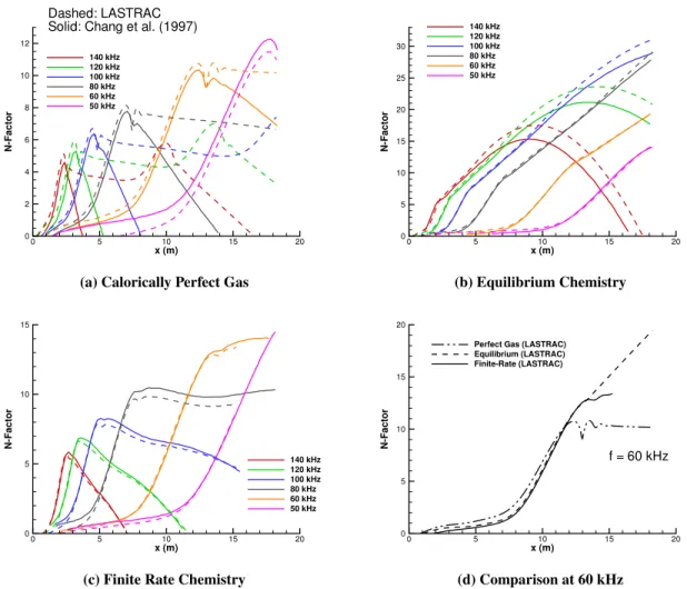
The second verification case is a sharp two-dimensional wedge with an angle of 6 degrees relative to the freestream in Mach 20 flow with a freestream unit Reynolds number of 9×10⁵per foot. The wall temperature is held constant with Tw/Tad =0.1, using the equilibrium adiabatic wall temperature for the finite-rate case. Consistent with the results in the literature, this is simulated as a flat plate with constant boundary layer edge conditions determined by the conditions after the shock calculated using Rankine-Hugoniot conditions. The post-shock edge Mach number is 12.5. Changes to the post-shock conditions due to changes to the gas model are not taken into account. Verification against results published by Chang et al. [3] are shown in Figure 3, showing the nonparallel N-factor calculated at a selection of frequencies. For the perfect gas, the current results show slightly higher peak N-factors and a smaller decaying rate past the peak. As will be shown later in Section B, supersonic modes emerge downstream of the peak second mode for this flow. Previous results appear to track the decaying second mode, while the present results capture the slowly decaying supersonic modes in the linear PSE solutions shown here. The small discrepancy in peak N-factor could be due to a slightly different Prandtl number and grids used in the boundary layer solutions. Despite these differences, the overall N-factor envelope seems to agree. Both chemical equilibrium and finite-rate results show good agreement with the reference results, with discrepancies in N-factor magnitude at some frequencies. These discrepancies may be due to differences in the mean flow set up and improved accuracy in discerning peak growth rates in the current work.
The third verification case is a sharp 10-degree half-angle cone at zero angle of attack with boundary layer edge conditions of Mach 11, edge temperature 1322 K, edge velocity of 7952 m/s, and edge pressure of 572 Pa based on Chang et al. [3]. For the calorically perfect gas, a constant ratio of specific heats (γ), can be set to match the temperature, velocity, and Mach number; however, for equilibrium and reacting cases,γis set by the chemistry model and the Mach number is slightly above 11. The wall temperature is held constant at 1200 K. To obtain the results shown, the Mach number was modified to produce results with edge velocities matching the reference case. These results are shown in Figure 4.
These verification results, over a range of conditions and a variety of simple geometries, give us a high degree of confidence that the necessary PSE and chemistry models are implemented correctly. Qualitative trends are matched well, and small quantitative differences are similar to the differences seen between results available in the literature.
V. Results
Results in this work, using the newly-implemented tools described in Section III, include an investigation of the effects of thermochemical nonequilibrium on a selection of the verification cases. This is followed by a study of supersonic modes on the Mach 20 wedge using perfect gas and finite-rate chemistry models, and an investigation of the effects of wall cooling on the same wedge. A hypersonic swept wing with a stationary crossflow instability is discussed
x (m) N -F a c to r 0 5 10 15 20 0 2 4 6 8 10 12 140 kHz 120 kHz 100 kHz 80 kHz 60 kHz 50 kHz Dashed: LASTRAC Solid: Chang et al. (1997)
(a) Calorically Perfect Gas
x (m) N -F a c to r 0 5 10 15 20 0 5 10 15 20 25 30 140 kHz 120 kHz 100 kHz 80 kHz 60 kHz 50 kHz (b) Equilibrium Chemistry x (m) N -F a c to r 0 5 10 15 20 0 5 10 15 140 kHz 120 kHz 100 kHz 80 kHz 60 kHz 50 kHz
(c) Finite Rate Chemistry
x (m) N -F a c to r 0 5 10 15 20 0 5 10 15 20
Perfect Gas (LASTRAC) Equilibrium (LASTRAC) Finite-Rate (LASTRAC)
f = 60 kHz
(d) Comparison at 60 kHz
Fig. 3 Nonparallel N-factor over a 6-degree wedge in Mach 20 flow compared to Chang et al. [3].
F x 103 -αi x 1 0 2 0.14 0.16 0.18 0.2 0.22 -0.2 -0.1 0 0.1 0.2 0.3 0.4 0.5 0.6 0.7
Chang et al. (1997), Perfect Gas Chang et al. (1997), Equilibrium Chemistry Chang et al. (1997), Finite-Rate Chemistry LASTRAC with Perfect Gas
LASTRAC with Equilibrium Chemistry LASTRAC with Finite-Rate Chemistry
using perfect gas and finite-rate chemistry models.
A. Investigation of Thermochemical Nonequilibrium on Verification Cases
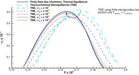
In order to test the implementation of the thermochemical nonequilibrium model, a mean flow solution for the cone from the third verification case was produced using the boundary layer flow solution for finite-rate chemistry in thermal equilibrium with the addition of the vibrational temperature equal to the translational temperature at every point. The results of this study are shown in Figure 5, where the vibrational-translational relaxation time is scaled to show that, as expected, as the relaxation time decreases the stability solution approaches that of the thermal equilibrium case. Using this case, where the mean flow is calculated assuming thermal equilibrium but thermal nonequilibrium is allowed in the disturbances, we can see that the existence of a nonzero relaxation time between vibrational and translational energy effects the stability of the boundary layer even when the mean flow is in thermal equilibrium. This indicates that it may be advantageous to include thermal nonequilibrium in boundary layer stability analysis even when the mean flow solution is unchanged by thermal nonequilibrium.
F x 103 -αi x 1 0 2 0.13 0.14 0.15 0.16 0.17 0.18 0.19 0.2 0 0.1 0.2 0.3 0.4 0.5
Finite Rate Gas Chemistry, Thermal Equilibrium Thermochemical Nonequilibrium (TNE) TNE, <τs > x 10-1 TNE, <τs > x 10-2 TNE, <τ s > x 10 -3 TNE, <τs > x 10-4 TNE, <τs > x 10-5
’TNE’ using finite-rate boundary layer solution and Tvibration = Ttranslation
Fig. 5 Growth rates at√Rex=982.7 on a sharp cone in Mach 11 flow, comparing thermochemical
nonequilib-rium and finite-rate models.
Using a mean flow solution for thermochemical nonequilibrium flow from VULCAN [38–40] on the two-dimensional wedge case, Figure 6 compares the PSE N-factor solution for all chemical models used in this work, at a disturbance frequency of 140 kHz. The thermochemical nonequilibrium results lie between the perfect gas and finite-rate chemistry results, with the third mode that was apparently damped out in the finite-rate solution reappearing at a further downstream location relative to the perfect gas as shown in Figure 6b. In Figure 6a, we can see that the 2ndmode is slightly stabilized by the inclusion of thermal nonequilibrium.
B. Supersonic Modes on the Mach 20, 6-Degree Wedge
Supersonic modes were identified for shear layers by Macaraeg and Streett [44]. Unlike other instability modes, the supersonic mode is associated with oscillations that occur outside the boundary layer region and may interact with the shock wave structure and be sensitive to the freestream conditions. This interaction with the flow outside of the boundary layer implies a greater degree of coupling between the disturbances growing in the boundary layer prior to transition with the bulk of the flow volume. The linear PSE N-factor distributions computed for the Mach 20 wedge case, shown in Figure 3, exhibit a kink after the peak of the second mode location for the perfect gas case. For the finite-rate case, the N-factor curve tends to level off or even goes up slightly beyond the second mode upper branch neutral point. As previously pointed out in Chang et al. [3], these unconventional tails of the second modes are associated with supersonic modes. Supersonic modes, in contrast to second-mode disturbances, travel with a phase speed less than
1
Me for the second mode disturbances, whereMeis the boundary layer edge Mach number. Both calorically perfect
x (m) N -F a c to r 0 2 4 6 8 2 4 6 8
Finite Rate Chemistry, CFD sol’n TNE, CFD sol’n
Finite Rate Chemistry, BL sol’n Equilibrium Gas, BL sol’n Perfect Gas, BL sol’n
(a) Close-in view to illustrate 2nd mode and possible supersonic modes. x (m) N -F a c to r 0 5 10 15 20 0 5 10 15 20
(b) Zoomed-out view to illustrate both 2nd and 3r d modes.
Fig. 6 Nonparallel N-factor over a 6-degree wedge in Mach 20 flow, with a 140 kHz disturbance.
these supersonic modes have relatively smaller growth rate than the peak second mode, but with a substantial region of growth near the end of the domain. The corresponding phase speed plot shown in Figure 7b confirms that these tail instability waves are indeed supersonic modes.
x(m) G ro w th R a te ( 1 /m ) 0 5 10 15 20 -1.5 -1 -0.5 0 0.5 1 1.5 2 2.5 Perfect Gas Finite Rate f=60kHz
(a) Growth rate comparison.
x(m) P h a s e S p e e d ( C r) 0 5 10 15 20 0.75 0.8 0.85 0.9 0.95 1 Perfect Gas Finite Rate f=60kHz Cr = 0.92
(b) Phase speed comparison, with line marking1−M1e.
Fig. 7 Comparisons between calorically perfect and finite-rate gas for a 60 kHz disturbance on a 6-degree wedge in Mach 20 flow.
It should be noted that finite-rate chemistry enhances growth but is not required for unstable supersonic modes. In addition, since the wall temperature boundary condition wasTw/Tadiabat ic =0.1, the results can be interpreted to mean that a ‘hot’ wall condition is not required for unstable supersonic modes to occur. Figure 8 shows the pressure perturbation structure for the finite-rate case caused when the unstable supersonic modes emit pressure waves outside of the boundary edge. The wave structure decays some distance away from the wall. The wave pattern shown in Figure 8 represents a typical wave structure for the growing supersonic modes.
x y 5000 10000 15000 20000 25000 30000 0 50 100 150 200 250 300 350 400 pressure perturbation: -40 -31 -22 -13 -4 4 13 22 31 40 f=60kHz, Finite Rate
Fig. 8 Pressure perturbation structure for finite-rate gas case of Mach 20, 6-degree wedge, for a 60 kHz disturbance. X and Y are nondimensionalized by`.
C. Wall Cooling Effects on the Mach 20, 6-Degree Wedge
In this section, a study comparing the effects of wall cooling for the perfect gas, equilibrium, and finite-rate chemistry models was performed on the Mach 20 6-degree wedge discussed in Section IV. Boundary layer codes were used to produce the mean flow results. The effect of wall temperature on boundary layer stability was discussed in the introduction, and to review, results in the literature show that while the first mode is stabilized by wall cooling, the second mode is destabilized. Since chemistry and temperature are tightly coupled, the inclusion of an appropriate chemical model is expected to affect the results. The relevance of this study to practical applications is to inform the choice of the most appropriate solution methodology when making design decisions such as the amount of active cooling used. If the inclusion of finite-rate chemistry shows a different trend or different magnitude of change in the transition location relative to the other models, then neglecting these effects could result in a design that has either under- or overestimated the cost of wall cooling. The results of this study show that, for a wall cooled well below the adiabatic wall temperature, a calorically perfect gas model would underestimate the change in transition point relative to a finite-rate chemical model, while a chemical equilibrium model would either under- or overestimate the change in transition point depending onNcr i t.
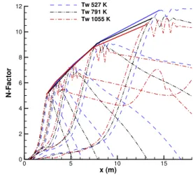
Figure 9a illustrates the PSE results for three chemical models with multiple wall temperatures at a single frequency, on the Mach 20 6-degree wedge. The coldest wall temperature used is 0.1 of the adiabatic wall temperature for an equilibrium chemistry model (0.1Tad ≈ 527K). The other wall temperatures used are at 0.15 and 0.2 of the equilibrium-gas adiabatic wall temperature. Although the adiabatic wall temperature would be different for the calorically perfect gas and thermally perfect finite-rate cases, the same temperature has been used in all three situations. From these results, we can see that while one effect of cooling is to shift the N-factor curve downstream, possibly delaying transition due to this single frequency, while another effect is that the peak N-factor has increased. This plots only includes a single frequency, and the trends predicted would only be expected where there is only a small range of frequencies of disturbance present inside the boundary layer, and where the N-factor curve at that frequency intersects Ncr i tprior to the peak N-factor. A more realistic assumption is that the freestream disturbances will take place at a broad spectrum of frequencies, and so we must look at the maximum N-factor over a range of frequencies as shown in Figures 9b– 9d. These plots confirm the conclusions found in the literature, that for hypersonic conditions, wall cooling has a destabilizing effect, causing the maximum N-factor curve to shift upstream and predicting an earlier transition point regardless ofNcr i t. For perfect and equilibrium gases shown in Figures 9b and 9c, the upstream shift in N-factors is more pronounced for low frequency disturbances that are dominating further downstream. Interestingly, for
the finite-rate chemistry case, the upstream shift prevails over a broad range of frequencies, if the transition N-factor is 10, then wall cooling would have the most impact on transition location if finite-rate chemistry is accounted for in this configuration. For the purposes of designing wall cooling to control transition on similar geometries, a perfect gas model may be sufficient for initial steps as the trend progresses in the same direction, however, a finite-rate model would be needed for a more accurate estimate of the change in transition location, and to achieve a design closer to the optimally delayed transition point. An equilibrium gas model should not be used for this purpose, as the value of the maximum N-factor as well as its slope differ much more from the finite-rate chemistry case. Although thermochemical nonequilibrium was not included in this study, this more inclusive model would be expected to produce more accurate results, which based on the results shown in Figure 6 would be expected to be similar to the finite-rate chemistry results since the maximum N-factor curve is most effected by the location of the second mode peak.
x (m) N -F a c to r 0 2 4 6 0 2 4 6 8 Tw 527 K Tw 791 K Tw 1055 K Equilibrium (blue)
Finite-Rate Chemistry (red)
Perfect Gas (black)
(a) Different gas models with disturbance frequency of 120 kHz. Line style indicates the temperature, while line color indicates the gas model.
x (m) N -F a c to r 0 5 10 15 0 2 4 6 8 10 12 Tw 527 K Tw 791 K Tw 1055 K
(b) A range of frequencies with calorically perfect gas assumed. Solid lines indicate an approximation to the maximum N-factor curve.
x (m) N -F a c to r 0 5 10 15 0 5 10 15 20 25 30 Tw 527 K Tw 791 K Tw 1055 K
(c) A range of frequencies with chemical equilibrium assumed. Solid lines indicate an approximation to the maximum N-factor curve.
x (m) N -F a c to r 0 5 10 15 0 2 4 6 8 10 12 14 Tw 527 K Tw 791 K Tw 1055 K
(d) A range of frequencies with finite-rate chemistry as-sumed. Solid lines indicate an approximation to the maximum N-factor curve.
D. Investigation of Stationary Crossflow Instability on a Hypersonic Swept Wing
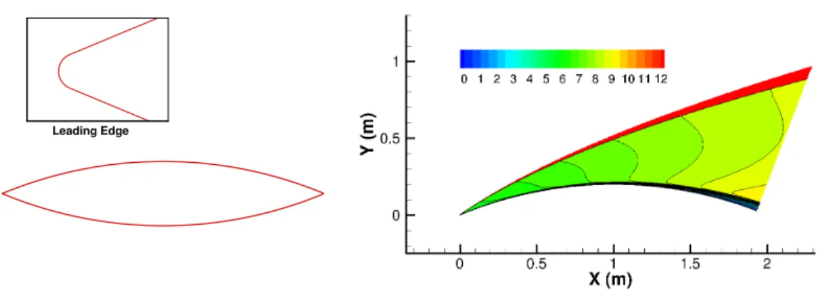
This section discusses a stationary crossflow instability on a swept wing in hypersonic flow, comparing the results between a calorically perfect gas and finite-rate chemistry. Results where the mean flow is generated using finite-rate chemistry while the stability analysis is conducted assuming a calorically perfect gas are also included. An infinite swept wing configuration was set up to generate a boundary layer that supports strong crossflow instability growth. An alternative candidate for this purpose may be a cone at an angle of attack, but the flow field associated with the cone is highly three-dimensional and is left for future studies. The flow field over a swept wing configuration, on the other hand, is essentially two-dimensional because there is no spanwise variation, and this can be addressed by the two-dimensional and axisymmetric options provided in LASTRAC, which are compatible with nonzero spanwise velocity. The existence of crossflow velocity in the boundary layer requires a streamwise pressure gradient. In the limit of a flat plate swept wing with a supersonic leading edge, the pressure over the wing chord is constant and hence there is no pressure gradient. Therefore, a symmetric circular-arc airfoil was created with a 20% thickness to chord ratio to ensure the existence of a large pressure gradient. The leading edge of the airfoil is a small circular arc with a 0.5mmradius that joins the main surface of the airfoil with continuous first derivative. The chord length is 2m, and the geometry is illustrated in Figure 10a. A wing with an infinite span was formed with the airfoil just described, with a 60 degree sweep angle.
A large freestream Mach number of 13 was used to ensure that chemical reactions take place on the wing that is placed at an angle of attack of -4 degrees. The freestream static pressure and static temperature are 1171.9 Pa and 226.6 K, respectively, corresponding to conditions at an altitude of 30,000m. The unit Reynolds number is 368,282/m. It should be emphasized that our purpose in creating this wing was to obtain a flow that supports strong crossflow instability growth, not for designing a wing that flies efficiently. The Mach contours are shown in a plane normal to the leading edge in Figure 10b. All crossflow instability computations were carried out on the upper surface of the wing where the pressure gradient is largest.
Leading Edge
(a) Circular-arc airfoil cross section. (b) Mach contours in a plane normal to the leading edge.
Fig. 10 Hypersonic swept with in Mach 13 freestream flow, at -4 degrees angle of attack.
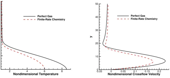
All mean flows in Section D were generated using VULCAN [38–40] and stability results were produced using LASTRAC for calorically perfect gas and finite-rate chemistry models. The inclusion of chemistry effects modifies the mean flow solution, changing the velocity, temperature, and pressure profiles. The species mass fractions now also have changing values throughout the boundary layer. Figures 11a and 11b illustrate the crossflow velocity and temperature profile differences between the perfect gas and finite-rate chemistry mean flow solution. The inclusion of chemical reactions has an endothermic effect, with a reduced adiabatic wall temperature due to the reduced ratio of specific heats in the chemically reacting case, and a reduction in the crossflow velocity magnitude. In this section, we also observe the effect of conducting stability analysis assuming a calorically perfect gas using a mean flow solution produced with a
finite-rate chemistry model. The goal of this is to investigate whether the change in instability is due to the change in mean flow alone, due to the effect of chemistry on the perturbations, or a mixture of the two.
Nondimensional Temperature y 2 4 6 8 0 10 20 30 40 50 Perfect Gas Finite-Rate Chemistry
(a) Temperature profiles nondimensionalized by bound-ary layer edge temperature.
Nondimensional Crossflow Velocity
y -0.050 0 0.05 0.1 0.15 0.2 10 20 30 40 50 Perfect Gas Finite-Rate Chemistry
(b) Crossflow velocity nondimensionalized by boundary layer edge velocity.
Fig. 11 Swept wing temperature and crossflow profiles at√Rex =1500, (x/chor d ≈0.3). Y coordinate is normalized by`.
Optimal growth wave angle results for both perfect gas and finite-rate chemistry models are shown in Figure 12. This plot identifies a stationary crossflow instability with the most amplified wave length being around 110mmfor the perfect gas model and the most amplified crossflow wave length being around 120mmfor the finite-rate chemistry model. The wave angles are nearly coincident for both cases. We can also observe that the growth rate is reduced for the finite-rate chemistry case.
Wave Length λ (m) -αi ( 1 /m ) W a v e A n g le ψ (d e g ) 0.05 0.1 0.15 0.2 0 2 4 6 8 10 12 87 87.5 88 88.5 89 Perfect Gas
Finite Rate Chemistry
Fig. 12 Growth rate and optimized wave angle versus crossflow wavelength in mm, at a constant√Rex=1500, (x/chor d ≈0.3), with f =0.
surface at a selection of crossflow wavelengths close to the most-amplified wavelengths previously found. In Figure 13, x/chord N -F a c to r 0 0.2 0.4 0.6 0.8 0 2 4 6 Perfect Gas LST Finite Rate LST 80 mm 60 mm 100 mm 120 mm 140 mm 160 mm
Fig. 13 Linear Stability Theory results on a hypersonic swept wing with a calorically perfect gas and thermally perfect finite-rate chemistry conditions.
we can see that the use of the finite-rate chemistry model has a stabilizing effect on the stationary cross-flow instability. The N-factors are lower, and transition would occur later on the surface, if at all, when finite rate chemical reactions are taken into account.
x/chord N -F a c to r 0 0.2 0.4 0.6 0.8 0 2 4 6 Perfect Gas LST Finite Rate LST
Finite Rate LST as Perfect Gas 60 mm 80 mm 100 mm 120 mm 140 mm 160 mm
(a) Parallel N-factors at a range of wave lengths.
x/chord N -F a c to r 0 0.2 0.4 0.6 0.8 0 2 4 6 Perfect Gas LST Finite Rate LST
Finite Rate LST as Perfect Gas
100 mm
(b) Parallel N-factors a wave length of 100 mm.
Fig. 14 Linear Stability Theory results on a hypersonic swept wing with calorically perfect gas and finite-rate chemistry conditions. Results using finite-rate chemistry mean flow and stability analysis using perfect gas assumptions are also shown.
From Figures 14a-14b, we can see that the stabilizing effect of chemistry comes from a combination of the new mean flow profile and from the new equations governing the perturbations. We conclude this from the way that the ‘finite-rate as perfect gas’ results lie part-way between the finite-rate and perfect-gas results. The ‘finite-rate as perfect gas’ case uses the mean flow evaluated assuming finite rate chemistry and stability equations assuming perfect gas, essentially neglecting the effects of chemical perturbations. The PSE method, unlike LST, includes the nonparallel effects of boundary layer thickness growth.
x/chord N -F a c to r 0 0.2 0.4 0.6 0.8 0 2 4 6 Perfect Gas, LST Perfect Gas, PSE
80 mm 60 mm
100 mm
120 mm
140 mm
(a) Calorically perfect gas.
x/chord N -F a c to r 0 0.2 0.4 0.6 0.8 0 1 2 3 4 5 6 Finite Rate, LST Finite Rate, PSE
60 mm 80 mm 100 mm 120 mm 140 mm (b) Finite-rate chemistry.
Fig. 15 LST compared to PSE for a hypersonic swept wing
These results also indicate that the inclusion of finite-rate chemistry effects is important to both the mean flow and the perturbations, with each contributing to the stabilizing effect on the boundary layer. Previous work by Chang [45] showed that cooling stabilizes crossflow modes through reducing the crossflow strength. Based on comparison of the mean flow results in Figure 11a, the inclusion of finite-rate chemistry has cooled the flow. The chemical reactions in this case have a net endothermic effect. Under conditions that lead to exothermic reactions a destabilizing effect would be expected.
VI. Summary and Conclusions
As a continual development effort for the NASA LASTRAC prediction tool set, chemical equilibrium, finite-rate chemical nonequilibrium, and thermochemical nonequilibrium have been implemented in LASTRAC for two-dimensional and axisymmetric geometries and the LST and linear PSE methods. These tools were used to investigate a variety of flow conditions and geometries, illustrating the 2nd and 3r dMack modes, supersonic modes, and the stationary crossflow instability.
The verification results presented in Section IV show that the new implementations of equilibrium, finite-rate chemistry, and thermochemical nonequilibrium models in LASTRAC are satisfactorily simulating the desired phenomenon. Further confirmation of the thermochemical nonequilibrium model may be included in future work. The implemented chemical and thermodynamic models are similar to that described by Gnoffo [28] and by Thompson et al. [21], and while more recent models exist, the choice of chemical model limits the potential differences between this work and the results in the literature used for verification. The code has been written in a modular way such that future modifications to the chemistry model will be straightforward, and such that it will be compatible with user-defined models in the future.
Using these newly implemented tools we compared thermochemical nonequilibrium results using first a finite-rate flow solution withTV =Tand showed that as the vibrational-electronic relaxation time decreases the stability results approach those obtained using thermally frozen finite-rate chemistry. Preliminary results show that the effect of thermochemical nonequilibrium on a 6-degree wedge was shown to be stabilizing to the 2nd mode and destabilizing to the 3r dmode relative to the finite-rate chemistry results. The supersonic modes observed on the wedge case were investigated further with comparisons between finite-rate chemistry and calorically perfect gas results, showing that supersonic modes exist for this case even for a calorically perfect gas, and that they are amplified by the inclusion of chemical reactions. The effect of chemistry with a net endothermic effect was seen to have a similar effect as cooling on a stationary crossflow instability on a swept wing in Mach 13 flow.