Coupled simulation of shock-wave/turbulent boundary-layer interaction over a flexible panel

Coupled simulation of shock-wave

/

turbulent boundary-layer

interaction over a flexible panel

V. Pasquariello†,1_{, S. Hickel}1,2_{and N. A. Adams}1

1_{Institute of Aerodynamics and Fluid Mechanics, Technische Universität München} Boltzmannstr. 15, D-85748 Garching

2_{Faculty of Aerospace Engineering}

Technische Universiteit Delft, Kluyverweg 1, NL-2629 HS Delft G. Hammerl3_{and W. A. Wall}3

3_{Institute for Computational Mechanics}

Technische Universität München, Boltzmannstr. 15, D-85748 Garching D. Daub4_{, S. Willems}4_{and A. Gülhan}4

4_{Institute of Aerodynamics and Flow Technology}

German Aerospace Center (DLR), Linder Höhe, D-51147 Cologne †_{Corresponding author, E-mail: vito.pasquariello@tum.de}

Abstract

We investigate the interaction of an oblique shock generated by a pitching wedge with a turbulent boundary-layer at a free-stream Mach number of Ma∞=3.0 and a Reynolds number based on the incoming boundary-layer thickness of Reδ0,I = 205⋅103. Large-eddy simulations (LES) are performed for two

configurations, that differ in the treatment of the wind-tunnel wall and shock generator movement within the experiment: A fixed panel with a static shock generator that deflects the flow byΘ = 20○, and the transient interaction of a pitching shock generator with an elastic panel. Besides mean and instantaneous flow quantities, we investigate unsteady aspects of the interaction region by means of wall-pressure spectra and provide comparison with experimental data whenever possible.

1. Introduction

Shock-wave/boundary-layer interactions (SWBLI) frequently occur in flows of technological interest, such as super-sonic air intakes, turbomachine cascades, helicopter blades, supersuper-sonic nozzles and launch vehicles in general. SWBLI can critically affect the vehicle or machine performance in several ways. The adverse pressure gradient acting on the flow strongly retards the boundary-layer, eventually leading to flow separation if the imposed pressure gradient is strong enough [5].

A schematic of the basic interaction type studied in this work is shown in Fig. 1. The adverse pressure gradient imposed by the incident shockC1is large enough to cause boundary-layer separation. Separation takes place well ahead of the inviscid impingementximp. The upstream propagation of the pressure gradient within the subsonic part of the turbulent boundary-layer (TBL) induces compression waves in the supersonic part of the TBL, which coalesce into the reflected shockC2. The reflected shock intersects the incident shock at pointIand the original shocks continue traveling as the transmitted shocksC3andC4, respectively. The shockC4penetrates into the separated shear layer, curves due to the local Mach number variation and finally reflects at the sonic line as an expansion fan. The separated shear layer, being primarily responsible for turbulence amplification, follows the inclination of the initial part of the separation bubble, while being deflected towards the wall due to the expansion fan and finally reattaching further downstream. The compression waves associated with reattachment merge to form the reattachment shockC5. Downstream of the SWBLI the TBL recovers an equilibrium state.

Until the 1950’s, SWBLI have been described as a steady process, which nowadays is known to be incorrect when shock-induced boundary-layer separation occurs. As stated by [6], the interaction region is the main source of maximum mean and fluctuating pressure levels as well as thermal loads. Turbulence production is enhanced in

Figure 1: Schematic of the oblique shock-wave/boundary-layer interaction with mean separation [15]. the vicinity of the mean separation location, which in turn increases viscous dissipation in this region [5]. The low-frequency unsteadiness of the reflected shock is a crucial aspect with regard to the choice of materials, since it is a main contribution to failure due to fatigue. [24] have shown that the separation acts as a broadband amplifier, for upstream distburbances.

In the context of launch vehicles, SWBLI are common flow features that may critically affect the rocket nozzle performance. During the start-up of liquid propellant fueled rocket engines, the rocket nozzle operates in an overex-panded condition, which leads to unsteady internal flow separation. The asymmetry of the separation and the inherent shock movement result in a net lateral force, which is often referred to as “side-load”. These high-magnitude transient loads can be severe enough to fail interfacing components as well as the complete nozzle in the rocket engine. Exper-imental tests of full-scale and sub-scale nozzles by [2] revealed a feedback mechanism between the unsteady SWBLI and one specific structural mode for a particular range of nozzle pressure ratios, resulting in a self-excited or aeroelas-tic vibration phenomenon. A comprehensive work on rocket nozzle flow separation and various side-load mechanisms can be found in [14]. With future rocket technologies focusing on optimal weight systems, fluid-structure interactions (FSI) become significant and must be taken into account in the design process in order to ensure the structural integrity. Multi-disciplinary numerical tools are necessary for a correct prediction of the complex flow physics influenced by structural deformations.

Within the collaborative research program “Transregio 40” (SFB-TRR 40) one objective is to develop high-fidelity numerical tools for an integrated interdisciplinary design process. For our studies we developed a Finite Volume – Finite Element coupling approach for the solution of compressible FSI problems based on a staggered Dirichlet-Neumann partitioning, where the interface motion within the Eulerian flow solver is accounted for by a cut-element based immersed boundary method [16]. Coupling conditions at the non-matching conjoined interface are enforced using a Mortar method.

Previous numerical studies concentrate on SWBLI with respect to a rigid surface [1, 7, 15] or deal with the aeroe-lastic response of eaeroe-lastic panels exposed to a laminar SWBLI [25]. To the authors knowledge, there is no high-fidelity large-eddy simulation (LES) available in the literature that deals with turbulent SWBLI coupled with a structural solver. In this study, we investigate the interaction of a TBL subjected to an adverse pressure gradient with a rigid and flexible panel. The adverse pressure gradient is generated by a pitching shock generator, inducing a time-varying pressure load on the panel, which subsequently leads to shock-induced flow separation and resembles typical overexpanded nozzle flow conditions. Besides mean and instantaneous flow quantities, we investigate unsteady aspects by means of wall-pressure spectra and the influence of the panel motion on turbulence.

Table 1: Flow parameters for the present studies.

Ma∞ T∞ p∞ δ0,Ia δ0,IIb Reδ0,I Reδ0,II

3.0 100.7 [K] 15.2 [kPa] 4.5 [mm] 5.2 [mm] 205_⋅103 _237⋅103

a.Evaluated atx=0.2 m b.Evaluated atx=0.26 m

2. Experimental setup

Experiments were conducted in the Trisonic Wind Tunnel (TMK) of the Supersonic and Hypersonic Technologies Department at DLR, Cologne. The TMK is a blow-down facility with a closed test section of 0.6×0.6 m. The

(a) 112 182 x y 87 300 220 1 . 47 30○ (b)

Figure 2: (a) Schematic of the experimental model. The baseplate consists of a fixed part (red) and an optional flexible insert (green). The shock generator is mounted on a shaft and spans the complete wind-tunnel width. (b) Two-dimensional sketch with main dimensions in millimeters.

continuously adjustable nozzle enables a Mach number range of Ma∞ = 0.5⋯4.5. Table 1 summarizes the flow conditions used for this investigation.

Figure 2(a) shows the setup that is used to validate our numerical tools. The interested reader is referred to [3, 4] for a detailed description. The test setup consists of a wedge mounted on a shaft that spans the complete wind-tunnel width, and of a baseplate with an optionally elastic part (green portion of the baseplate in Fig. 2(a)) for FSI experiments. The baseplate has the same width as the wind-tunnel test section. Main dimensions are given in Fig. 2(b). For the FSI configuration, a frame is inserted into the baseplate, which carries an elastic panel made of 1.47 mm thick spring steel (CK 75). It has a length of L = 300 mm and width of W = 200 mm. Two rows of rivets at the front side (x∈ [205,220]mm) as well as at the rear side (x∈ [520,535]mm) of the elastic panel are used to fix the panel with the surrounding frame. In spanwise direction the panel motion is not restricted. A cavity below the panel carries measurement instrumentations. It is sealed through a thick layer of a soft foam rubber, applied between the underside of the elastic panel and the frame. Pressure equalization of the cavity is done at a point upstream of the interaction, resembling undisturbed free-stream conditions. Boundary-layer tripping is applied behind the leading edge to ensure a fully developed TBL.

In order to ensure well-defined initial conditions for both fluid and solid subdomain for the FSI configuration, the initial position of the wedge is chosen in such a way that the generated shock-wave does not impinge on the elastic panel, yielding a sufficiently undeformed and unstressed structure. In case of FSI experiments, the wedge is pitched fromΘt0 =0○toΘt1 =17.5○in approximately Trot=15 ms, inducing a time-varying load on the plate with significant

boundary-layer separation. For the baseline uncoupled configuration, the static shock generator deflects the flow by

Θ=20○.

3. Numerical approach

The governing equations for the fluid domain are the compressible Navier-Stokes equations. The Adaptive Local Deconvolution Method (ALDM, [9, 10]) is used for the discretization of the convective fluxes and provides a physically consistent subgrid-scale turbulence model for implicit LES. Employing a shock sensor to detect discontinuities and switch on the shock-dissipation mechanism, ALDM can capture shock waves while smooth waves and turbulence are propagated accurately without excessive numerical dissipation [10]. The diffusive fluxes are discretized using a 2nd

order central difference scheme, and a 3rd_{order Runge Kutta scheme is used for the time integration. The flow solver}

operates on Cartesian grids for a high parallel performance. The elastic wall boundary is represented by a cut-element immersed boundary method [13, 16].

The structural field is governed by the weak form of the linear-momentum balance, describing equilibrium of the forces of inertia, internal and external forces. A hyperelastic Saint Venant-Kirchhoffmaterial model is chosen. The structural field is discretized with the Finite Element method. The fully discrete nonlinear structural system is solved iteratively by a Newton-Raphson method. The method of enhanced assumed strains (EAS) is used in order to avoid locking phenomena. For time integration, the generalized trapezoidal rule (or one-step-θscheme) is employed.

We make use of a classical Dirichlet-Neumann partitioning in conjunction with a Conventional Serial Staggered procedure for coupling of the two domains. Our framework [16] inevitably leads to a non-matching discretization of the interface between both subdomains. Load transfer is established by a consistent Mortar method, which preserves linear and angular momentum. In order to resolve the different time-scales of both subdomains and increase the overall

efficiency, subcycling within the fluid domain is used. The chosen subcycling time-step is∆ts = 2⋅10−6s, which

on the one hand leads to a sampling factor of 2250 with respect to the first structural eigenfrequency found in the experiment (f1 = 222 Hz) and on the other hand guarantees that high-frequency fluctuations associated to the TBL (fTBL=δ0,I/U∞=7.5⋅10−6s) are still resolved.

4. Computational setup

The origin of the coordinate system used for our studies is placed at the sharp leading edge of the baseplate, see Fig. 2(b). For the baseline SWBLI, the computational domain is rectangular with dimensionsLx=55δ0,I,Ly=11δ0,I,

Lz = 2δ0,I and it is discretized with 1800 × 460 × 128 cells in streamwise, wall-normal and spanwise directions,

respectively. This leads to a grid resolution of△x+=42,△y+min=1,△z+=21 evaluated at the origin of the LES domain

(x=0.2 m). In the wall-normal direction hyperbolic grid stretching is used with a stretching factor ofβy=3.0, where

the stretching function readsy=Ly(1−tanh(βy(1−j/Ny)) /tanh(βy)). Here, jdenotes the individual grid point,Ly

the domain height andNythe total number of cells in wall-normal direction. The following boundary conditions have

been used for the LES. At the domain inlet a Digital Filter (DF) based boundary condition is used [23], for which first and second order statistical moments have been obtained through a precursor temporal boundary-layer simulation at the same flow conditions. This type of boundary condition omits the introduction of artificially correlated data, which would potentially force low-frequency periodic motion of the reflected shock. At the top boundary, flow conditions are adopted from an inviscid simulation atΘ=20○_{wedge angle and interpolated onto the target grid. This guarantees the} correct interaction of the incident shock and the expansion fan originating from the static shock generator. The nominal inviscid impingement point at the wall isximp=0.307 m, neglecting the influence of the expansion fan on the incident

shock. At the supersonic outlet, linear extrapolation of all flow variables is used. The wall is modeled as adiabatic and periodic boundary conditions are used in the spanwise direction. Statistical quantities have been obtained by averaging instantaneous three-dimensional flow fields in time and spanwise direction after an initial transient of 5Lx/U∞and at a mean sampling time of 0.04δ0,I/U∞, resulting in a total of 57200 samples within the available integration time. For the low-frequency analysis presented later, 1008 equally spaced pressure probes have been placed in streamwise direction along the wall (y=0) ranging betweenx=0.24 m andx=0.38 m.

Considering the FSI setup, the LES domain starts fromxmin=0.17 m and ranges up toxmax=0.57 m in

stream-wise direction, thus covering the complete elastic panel section (see Fig. 2(b)). This corresponds to a domain length ofLx = 88δ0,I. In spanwise direction, the same domain width as for the baseline case ofLz =2δ0,I is used, which

implicitly assumes a two-dimensional FSI. In order to account for the panel motion within the Cartesian flow solver, a cavity of height 5 mm is used within the elastic panel section. Thus, in wall-normal direction the domain covers the sectionymin= −0.005 m up toymax=0.1 m, leading toLy=23δ0,I. To reduce the overall amount of computational cells,

we first performed inviscid FSI simulations to identify the region of panel motion. Subsequently, the cavity is split into several smaller blocks and those which remain uncut within the whole simulation time have been deleted. In total, the computational grid comprises 79.56_⋅106_{cells, with a final grid resolution expressed in wall-units of△x}+ _{= 62,}

△y+min=5,△z+=30. The same grid stretching strategy has been used for the boundary-layer block as for the baseline

configuration, whereas a uniform grid spacing is used within the cavity region in order to ensure the same wall resolu-tion throughout the whole simularesolu-tion time. The boundary condiresolu-tions for the fluid subdomain are the same as the ones described beforehand, with the only difference that at the top of the domain a transient boundary condition has been implemented, which prescribes pre-shock, post-shock and expansion states at each individual grid position according to the experimental time-dependent wedge angle.

The panel is discretized using 200 ×2 ×12 tri-linearly interpolated hexahedral elements in streamwise, wall-normal and spanwise direction, respectively. To avoid shear locking phenomena, the EAS method is used. The panel has a Young’s modulus ofES = 206 GPa, a Poisson’s ratio of νS = 0.33, and a density ofρS;0 = 7800 kg/m3. No perfectly clamped boundary condition is achieved in the experiment. Both, the rivets as well as the frame to which the panel is connected deform, which in turn leads to larger wall-normal deformations of the panel [26]. In order to account for this effect, elastic boundary conditions with linear springs at both ends of the panel are used. A spring constant ofklin =4.15⋅108N/m is used, which has been calibrated using results of experiments during which the panel was

exposed to a constant pressure difference (see Fig. 11(b)). At the bottom surface of the panel, a time-dependent cavity pressure extracted from the experiment is imposed. A coupled simulation is started by first assuming a rigid panel. After one flow-through time (FTT) of the TBL, the rigidity constraint is removed and the coupled simulation starts. Before the pitching of the shock generator is enabled, the whole system is integrated for again one FTT to reduce the influence of initial transients on the later panel motion.

2

3

4

5

6

0

1000 2000 3000 4000 5000

h

C

i

·

10

Re

1

2

3

4

5

6

0

50

100

150

200

y

[mm]

p

[kPa]

Figure 3: (a) Incompressible skin friction evolution. (–●–) Blasius; (–▾–) Kàrmàn-Schoenherr; (—) Smits; (—) LES;

(D) [18]; (●) [17]; (⊙) [11],△[20]; (▽) [22], (◇) CAT5301 AGARD 223, (+) [8], (×) [12]. (b) Wall-normal total pressure distribution atx=0.15 m. The LES pressure distribution has been corrected according to the Rayleigh Pitot tube formula, see Eq. (1). (—) LES, (●) experimental data.

5. Results and discussion

The spatial extent of the separation bubble is sensitive on the level of turbulence in the incoming TBL. Thus, be-fore the SWBLI simulations are considered, a spatially developing TBL simulation without shock generator has been conducted, which covers the experimental Pitot rake position located atx=0.15 m.

Since no direct measurement of the skin-friction is available for this flow configuration, the incompressible skin friction distribution_⟨Cfi⟩obtained from the van-Driest II transformation is compared to algebraic incompressible

relations, various DNS and experimental data for a wide range of Mach numbers; see Fig. 3(a). The computed incom-pressible skin friction coefficient (—) is in good agreement with the DNS results by [17]. In Fig. 3(b), we provide a comparison between experiment and LES in terms of ram-pressure measured at the streamwise locationx= 0.15 m. In order to account for the shock-losses generated by the Pitot rake, the LES pressure is corrected according to the Rayleigh Pitot tube formula

pt p = [ ( γ+1)2_Ma2 4γMa2_−2(γ−1)] γ/(γ−1) ⋅1−γ_γ+₊2γMa₁ 2, (1)

where Ma denotes the local Mach number. The good agreement between experiment and LES confirms the correct boundary-layer thickness evolution within the simulation and justifies the assumption of a fully TBL.

For further validation, the van-Driest transformed mean-velocity profile together with the RMS of Reynolds stresses in Morkovin scaling at the same streamwise positionx=0.15 m are presented in Fig. 4(a)/(b) and compared with DNS data of [17] for a similar friction Reynolds number (Reτ,LES=840,Reτ,DNS=900). Note that the DNS has a different Mach number of Ma∞=2.0 and a lower local Reynolds number of Reδ,DNS =55170. The velocity profile is in good agreement with the logarithmic law of the wall and the DNS data. Small differences in the wake region are due to a higher Reynolds number in the LES. The Reynolds stresses are in good agreement with the DNS data in the near-wall region, while larger deviations occur in the logarithmic and wake region.

5.2 Baseline SWBLI atΘ=20○

The baseline SWBLI considers the experimental configuration with a static shock generator, which deflects the flow byΘ= 20○. Contours of the instantaneous and time-averaged temperature, see Fig. 5, give a first impression of the flow topology. The sonic line is shown in black and zero streamwise velocity is shown in blue. The adverse pressure gradient imposed by the incident shock is strong enough to cause a massive boundary-layer separation. The same flow

0

5

10

15

20

25

10

10

10

10

h

u

i

y

-1

0

1

2

3

10

10

10

10

p

h

ρ

i

/ρ

·

r

h

u

u

i

y

Figure 4: (a) van-Driest transformed mean-velocity profile atx=0.15 m (Reτ=840). (b) RMS of Reynolds stresses

with density scaling atx=0.15 m (Reτ=840). (—) LES, (●) DNS data at Ma=2.0 and Reτ=900 from [17]

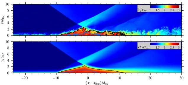
T/T∞ 1 1.5 2 2.5 3 y / δ0, I 2 4 6 8 10 0 ⟨T⟩/T∞1 1.5 2 2.5 3 (x−ximp)/δ0,I −20 −10 0 10 20 30 y / δ0, I 2 4 6 8 10 0

Figure 5: Top: Instantaneous temperature distributionT/T∞inx−ymid-plane. Bottom: Time- and spanwise-averaged temperature distribution⟨T⟩/T∞. (—) Ma=1, (—)u=0.

features as described in Fig. 1 can be identified. Moreover, the contour plot clearly highlights a heating process of the fluid within the recirculating region.

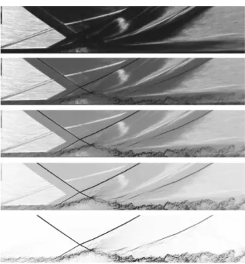
A qualitative comparison between experiment and simulation is given in Fig. 6, where we show instantaneous schlieren pictures. The opacity of the fluid solution is decreased from top to bottom. Qualitatively, one can observe a good agreement in terms of the separation shock angle, the extent of separated flow, the thickening of the TBL after the SWBLI and the evolution of the detached shear layer. Note that due to the interaction of the incident shock with the wind-tunnel side-wall TBL, the incident and separation shock within the experiment appear smeared. This is not the case for the LES due to the periodic boundary conditions applied in spanwise direction. However, as will be shown later in conjunction with the wall-pressure evolution (Fig. 7), this effect does not affect the interaction near thex−y mid-plane.

The mean skin friction evolution is shown in Fig. 7(a). The synthetic turbulence generator leads to a spatial transient close to the inflow, wherein the flow recovers modeling errors introduced by the DF procedure. Due to the adverse pressure gradient imposed on the TBL, the flow is decelerated and forms a recirculation zone as indicated by the change of sign in the friction coefficient ⟨Cf⟩. The mean separation length for the baseline configuration is

Lsep=13.11δ0,I. The effect of the shock generator trailing-edge expansion fan on the interaction is clearly visible. After

Figure 6: Instantaneous schlieren comparison between LES and experiment for the static SWBLI case atΘ = 20○ deflection angle. The opacity of the fluid solutions is decreased from top to bottom. The LES schlieren is evaluated at thex₋ymid-plane.

the effect of decreasing skin friction due to a thickening of the TBL dominates and⟨Cf⟩starts to decrease.

The wall-pressure evolution is shown in Fig. 7(b) for experiment and LES. The experimental data has been evaluated at the mid-plane and is time-averaged, while the LES data has been both time- and spanwise-averaged. Besides experimental data points from static pressure probes (_●), we also provide the mean pressure extracted from unsteady pressure measurements through eight Kulites (_▵). The pressure increase associated with the impinging shock is felt approximately 10δ0,I before the theoretical inviscid impingement location ximp, also known as the upstream influence mechanism [5]. Within the initial part of the separation bubble (xs<x<ximp), a significant pressure plateau can be observed, indicating the presence of a strong interaction, followed by a monotonically increasing pressure associated to the reattachment process. The trailing-edge Prandtl-Meyer expansion leads to a strong pressure drop after the SWBLI. Numerical and experimental data for the pressure evolution are in excellent agreement, confirming the ability of our LES solver to correctly predict SWBLI at high Reynolds numbers. In particular, the pressure plateau is captured well, indicating that the present experimental setup is sufficiently two-dimensional and accessible through LES with assumed homogeneity in spanwise direction.

The influence of the SWBLI on turbulence evolution is studied in Fig. 8 in terms of mean resolved Reynolds shear stress (top) and turbulence kinetic energy (bottom). The mean sonic line (black) and the separated flow region (red) are highlighted. A high level of Reynolds shear stress is found along the detached shear layer within the interaction region. Its maximum value is found approximately one boundary-layer thickness downstream of the mean reattachment location, consistent with previous findings for different flow conditions [15, 19]. In addition, high levels of⟨u′v′⟩can be observed along the reflected (C2,C3) and reattachment (C5) shock, being directly associated with unsteady shock motions and coupled to a breathing motion of the separation bubble [7]. At the incident shock tip (C4),⟨u′v′⟩changes sign as a consequence of its flapping motion [21]. The mean resolved turbulence kinetic energy contour confirms amplification of turbulence along the shear layer that originates from the separation point.

Unsteady aspects related to reflected shock dynamics are investigated by means of Power Spectral Densities (PSD) of wall-pressure probes. Pressure signals have been recorded at a mean sampling time interval of 8_⋅10−4_δ

0,I/U∞ covering a length of 1900δ0,I/U∞. This leads to a maximum resolvable Strouhal number of Stmax = fmaxδ0,I/U∞ = 625 and a minimum resolvable Strouhal number of Stmin = fminδ0,I/U∞ = 5⋅10−4. Consequently, the current LES is well able to capture the expected low-frequency unsteadiness. Fig. 9 provides a two-dimensional map of wall-pressure spectra evaluated at each streamwise wall-pressure-probe location. The spectra have been obtained using the Welch algorithm by splitting the signal in three segments with 50 % overlap using Hanning windows. Each pre-multiplied PSD contour has been normalized, such that their integral over frequency becomes unity, i.e. f⋅PSD(f_{)/ ∫} PSD(f)df. This normalization has the favorable effect to highlight frequencies that contribute most at each individual streamwise

−

1

−

0

.

5

0

0

.

5

1

1

.

5

2

2

.

5

3

−

20

−

10

0

10

20

30

h

C

i

·

10

(

x

−

x

)

/δ

1

2

3

4

5

−

20

−

10

0

10

20

30

h

p

i

/p

(

x

−

x

)

/δ

Figure 7: (a) Skin friction⟨Cf⟩(b) and wall-pressure⟨pw⟩/p∞evolution in the streamwise direction. (—) LES, (●)

experimental static data, (▵) experimental Kulite data. Kulite positions Ki∣i=1...8are highlighted for later reference.

−⟨u′v′⟩ u2 ∞ ⋅10 −3 −5 0 5 10 15 y / δ0, I 2 4 6 8 10 0 0 9.5 19 28.5 38 (x−ximp)/δ0,I −20 ₋10 0 10 20 30 y / δ0, I 2 4 6 8 10 0 ⟨u′iu′i⟩ 2u2 ∞ ⋅10 −3

Figure 8: Top: Mean resolved Reynolds shear stress. Bottom: Mean resolved turbulence kinetic energy. (—) Ma=1,

(—)u=0.

location. The PSD map shows a broadband peak centered around unity Strouhal number before separation takes place (x< xs), being directly associated to the characteristic frequency of energetic scales within the incoming TBL (U∞/δ0,I). The energy peak shifts towards significantly lower frequencies in the vicinity of the mean separation location

and moves back again to higher frequencies downstream of the interaction zone. Due to a thickening of the TBL after the SWBLI, the broadband peak shifts to overall lower Strouhal numbers. The low-frequency peak close to the mean separation location is related to the back and forth motion of the reflected shock and covers a streamwise shock-excursion length of about one boundary-layer thickness, consistent with previous findings [7, 15]. A characteristic Strouhal number of StLsep=0.08 based on the mean separation lengthLsepis found for the low-frequent shock motion.

A total number of 12 low-frequency cycles is captured within the available integration time.

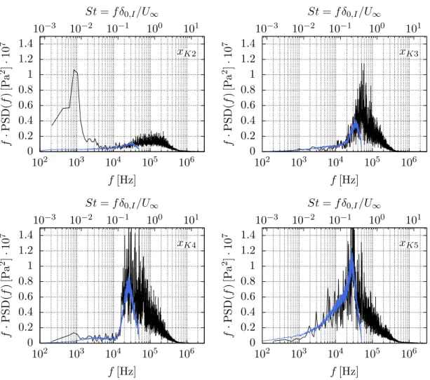
Selected PSDs at the Kulite positionsxK2. . .xK5are compared to experimental data, see Fig. 10. Each Kulite has 550000 data points at a sampling frequency of 100 kHz. For the experimental PSDs, the signal is split in 50 segments with 50 % overlap using Hanning windows, which leads to a smooth spectrum compared to the ones obtained for the LES. The Kulites have a diameter of 1.7 mm and cover several LES wall-pressure probes. Therefore, LES spectra corresponding to the same Kulite position have been averaged. For the first Kulite position,xK2, the LES reveals an

energetically dominant low-frequency peak which is not present in the experiment. From Fig. 7 it is evident, that xK2perfectly matches the mean separation location predicted by the LES, thus explaining the low-frequency peak in

−14 −12 −10 −8 −6 −4 −2 0 2 4 6 8 10−2 10−1 100 S t = f δ0, I / U∞ 0 0.1 0.2 0.3 0.4 0.5 xs ximp xr (x₋ximp)/δ0,I

Figure 9: Weighted power spectral density map extracted from all wall-pressure signals for the baseline configuration. Contour: f⋅PSD(f_{)/ ∫} PSD(f)df.

0

0

.

2

0

.

4

0

.

6

0

.

8

1

1

.

2

1

.

4

10

10

10

10

10

10

10

10

10

10

f

·

PSD(

f

)

[P

a

]

·

10

f

[Hz]

St

=

f δ

/U

x

0

0

.

2

0

.

4

0

.

6

0

.

8

1

1

.

2

1

.

4

10

10

10

10

10

10

10

10

10

10

f

·

PSD(

f

)

[P

a

]

·

10

f

[Hz]

St

=

f δ

/U

x

0

0

.

2

0

.

4

0

.

6

0

.

8

1

1

.

2

1

.

4

10

10

10

10

10

10

10

10

10

10

f

·

PSD(

f

)

[P

a

]

·

10

f

[Hz]

St

=

f δ

/U

x

0

0

.

2

0

.

4

0

.

6

0

.

8

1

1

.

2

1

.

4

10

10

10

10

10

10

10

10

10

10

f

·

PSD(

f

)

[P

a

]

·

10

f

[Hz]

St

=

f δ

/U

x

Figure 10: Weighted power spectral density at streamwise locations associated to experimental Kulite positions xK2. . .xK5, see Fig. 7 for reference. (—) LES, (—) experiment.

0

4

8

12

16

20

0

5

10

15

20

25

14

.

5

15

15

.

5

16

16

.

5

17

17

.

5

Θ

[

]

p

[kP

a]

t

[ms]

−

6

−

4

−

2

0

0

10

20

30

40

50

∆

y

[mm]

∆

p

[kPa]

−

6

−

5

−

4

−

3

−

2

−

1

0

1

0

0

.

005

0

.

01

0

.

015

0

.

02

∆

y

[mm]

t

[s]

Figure 11: (a) Experimental parameters of the coupled setup: (_{− ⋅ −}) deflection angleΘmeasured with respect to the horizontal axis, (_⋯) cavity pressurepcav, (—) approximated pressure load for the structural model. (b) Calibration of the linear springs: (—) static deflection withklin =4.15⋅108N/m, (●) experimental data. (c) Deflection of the panel

mid-node over time. Mean static deflection and characteristic frequencies are highlighted. (—) LES, (—) experiment.

the associated PSD. However, the experimental mean separation location is probably located 1.5δ0,I upstream ofxK2.

Since the shock-excursion length is assumed to be around 1δ0,I, see Fig. 9, Kulite 2 probably misses the low-frequent

shock motion. Besides this discrepancy, the high-frequency energy content is very similar between experiment and LES for the remaining Kulite positions. Moreover, the steep gradient found forxK4close to St=0.1 is captured very well by the LES.

5.3 Coupled SWBLI at⟨Θ⟩ =17.5○

The coupled SWBLI considers the experimental configuration with a pitching shock generator and a final mean deflec-tion angle of_⟨Θ⟩ =17.5○_{. Fig. 11(a) summarizes experimental parameters. WithinT =15 ms, the wedge is pitched} fromΘt0=0○toΘt1=17.5○, inducing a time-varying load on the plate. Att=3 ms, the incident shock hits the end of

the panel. The nominal mean inviscid impingement location isximp=0.328 m. Note, that low-amplitude oscillations of the shock generator at a frequency offSG≈247 Hz are still visible after the transient pitching. The time-varying wedge angle is used for the LES to prescribe a transient boundary condition at the top of the domain. In the same figure, the experimental cavity pressurepcavis shown. No perfect sealing between the main stream and the cavity below the panel can be achieved in the experiment, thus leading to a pressure increase inside the cavity once the shock hits the panel. In order to account for the increased pressure in the cavity, a simplified pressure curve is assumed, which is imposed

(x−ximp)/δ0,I −20 −10 0 10 20 30 y / δ0, I 2 4 6 8 10 0

Figure 12: Instantaneous schlieren of the coupled LES evaluated at the mid-plane att=16.46 ms.

−20 −10 0 10 20 30 40 0 5 10 15 20 xp,0 xp,L (x−ximp)/δ0,I t [ ms ] p / p∞ 1 2 3 240 Hz 186 Hz

Figure 13: x−tdiagram of recorded pressure aty=0 evaluated at the mid-plane. Panel startxp,0and panel endxp,L

are indicated.

as a time-dependent Neumann boundary condition, see solid black line in Fig. 11(a). Actually, the pressure is coupled to the panel deflection, which is neglected in the present setup. Fig. 11(b) shows results after calibration of the linear springs with a spring constant ofklin=4.15⋅108N/m, indicating an overall good agreement between experiment and

simulation in terms of static deflections. The deflection of the panel mid-node over time for the coupled SWBLI is shown for both experiment and LES in Fig. 11(c). Mean static deflection and characteristic frequency of the panel oscillation are indicated. Within 7_<t_<11 ms, the panel displacement increases linearly, followed by an oscillatory behavior. A mean static deflection of∆yLES = −3.77 mm is found for the LES, which is in excellent agreement with the experimental value of∆yEXP = −3.85 mm. Considering the time-evolution of the panel displacement, an overall good agreement can be observed for the initial pitching region (t < 11 ms), whereas larger deviations occur at the onset of panel oscillations. Both, the frequency of the panel oscillation (fLES=186 Hz, fEXP=222 Hz) as well as the displacement amplitudes differ significantly from the experiment. The authors believe, that the compressible air within the cavity constitutes an additional stiffness which is not included in our setup, but could be possibly modeled through an additional set of springs acting on the underside of the elastic panel. This would in turn increase the frequency of the panel oscillation and explain the current mismatch between experiment and simulation. Regarding the oscillation amplitudes, a relatively high damping is observed in the experiment, which is not the case for the LES. The authors believe, that two effects are mainly responsible for this discrepancy: The cavity is sealed through a thick layer of a soft foam rubber, which may increase the overall damping of the system and leads to a damping effect that scales linearly with the panel velocity. The second reason is attributed to the aerodynamic damping imposed by the cavity, which is expected to scale with the square of the panel velocity. As it is not yet clear how to model this damping behavior cor-rectly, more experiments are necessary for modeling purposes. Therefore, damping in the structural model is neglected in the current numerical setup.

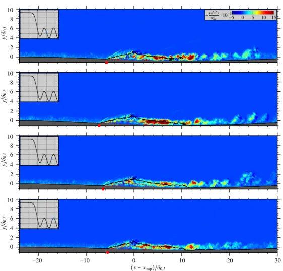
y / δ0, I 2 4 6 8 10 0 (x−ximp)/δ0,I −20 −10 0 10 20 30 −⟨u′v′⟩ u2 ∞ ⋅10 −3 −5 0 5 10 15 y / δ0, I 2 4 6 8 10 0 y / δ0,I 2 4 6 8 10 0 y / δ0, I 2 4 6 8 10 0

Figure 14: Resolved spanwise-averaged Reynolds shear stress for selected snapshots (—) Ma = 1, (—) u = 0.

(xp,0−ximp)/δ0,I= −23.89,(xp,L−ximp)/δ0,I =42.48. Red bullets indicate the instantaneous separation shock

loca-tion.

flow features can be identified when compared to the baseline configuration (Fig. 6), with the only difference being a large mean static deflection of the order of one δ0,I. Equally spaced pressure probes have been placed in streamwise

direction along the undeflected panel (y=0) ranging betweenx=0.22 m andx=0.52 m. The recorded pressure for the coupled SWBLI is shown in Fig. 13 in terms of ax−tdiagram. Panel startxp,0and panel endxp,Lare indicated.

Starting fromt=3 ms, the panel is exposed to an increasing pressure force. Boundary-layer separation can be observed fort_>8 ms with growing spatial extent up tot₌15 ms. Fort_>15 ms, a quasi-stationary state of the coupled SWBLI is obtained. Compression and expansion waves emanating from the panel oscillation (fLES=186 Hz) can be clearly seen in the rear part of the panel. A large-scale separation shock movement can be observed atx−ximp ≈ −6δ0,I, probably

caused by the oscillating incident shock, see Fig. 11(a). We found a frequency of 240 Hz for the large-scale separation shock movement, which is closely related to the shock generator oscillation frequency, being 247 Hz. At the same time, the reattachment shock (x−ximp≈4δ0,I) exhibits an opposite motion, which constitutes an overall breathing motion of

the separation bubble.

Four selected spanwise averaged snapshots with contours of resolved Reynolds shear stress are shown in Fig. 14. The snapshots are taken in the time intervalt∈ [15.1,19.1]ms, representing one oscillation period within the quasi-stationary state. Each insert shows the panel deflection evaluated at the mid-node together with a blue bullet, which indicates the associated snapshot time. The sonic line is shown in black and zero streamwise velocity is shown in red. The reflected shock foot is tracked with a red bullet. The large-scale shock motion discussed in conjunction with Fig. 13 is clearly visible and covers a maximum excursion length of approximately 2δ0,I.

A comparison between the baseline SWBLI and the coupled configuration is given in Fig. 15 in terms of time-and spanwise-averaged resolved Reynolds shear stress. The coupled results have been averaged over one oscillation period (t∈ [15.0,20.3]ms) with a total number of 165 samples, explaining the noisy contours compared to the baseline setup. Compared to the uncoupled case, the separation, reflected and reattachment shock exhibit a low-frequent shock

−⟨u′v′⟩ u2 ∞ ⋅10 −3 −5 0 5 10 15 y / δ0, I 2 4 6 8 10 0 (x−ximp)/δ0,I −20 −10 0 10 20 30 y / δ0, I 2 4 6 8 10 0

Figure 15: Time- and spanwise-averaged resolved Reynolds shear stress. Top: Baseline SWBLI at⟨Θ⟩ =20○. Bottom: Coupled SWBLI at⟨Θ⟩ =17.5○. (—) Ma=1, (—)u=0. The coupled results have been averaged over one oscillation

period. 1 2 3 4 5 −20 ₋10 0 10 20 30 40 h pw i /p∞ (x₋ximp)/δ0,I

Figure 16: Wall-pressure⟨pw⟩/p∞evolution in the streamwise direction. (—) coupled SWBLI at⟨Θ⟩ =17.5○, (—)

baseline SWBLI at⟨Θ⟩ =20○. The coupled results have been averaged over one oscillation period.

motion with greater spatial extent, probably caused by a superposition of the oscillating incident shock and the panel motion. The mean separation length is approximately 2δ0,I smaller for the coupled SWBLI. One must keep in mind

that a direct comparison between both cases is not possible, since different mean deflection angles are considered. As a consequence, both, the smaller mean deflection angle and a negative static displacement of the panel contribute to an overall weaker interaction.

Finally, Fig. 16 shows the mean wall-pressure evolution for both cases. The mean deflection of the panel leads to an overall lower pressure level before the interaction region (x−ximp< −10δ0,I), indicating the presence of expansion

waves which accelerate the near-wall flow. This effect in turn contributes to an overall reduced interaction length. As already explained in conjunction with Fig. 15, a weaker mean SWBLI is present for the coupled SWBLI. Thus, a superposition of both effects leads to a lower pressure plateau and lower maximum pressure increase across the interaction.

6. Conclusions

We have studied the interaction of an oblique shock with a turbulent boundary-layer (TBL) using well-resolved large-eddy simulation (LES) and experimental data. The flow is deflected by a rotatable shock generator at a free-stream Mach number of Ma = 3.0. The Reynolds number upstream of the interaction region isReδ0,I = 205⋅103. Two

configurations have been investigated: The first one considers a steady shock generator with a deflection angle of

Θ= 20○. The second setup investigates the fluid-structure interaction (FSI) arising from a pitching shock generator, whose incident shock interacts with a flexible panel.

The validity of the incoming TBL has been assessed through a direct comparison between LES results and data from direct numerical simulation found in the literature. An overall good agreement could be found in terms of van-Driest transformed mean velocity, Reynolds stresses and incompressible skin-friction evolution. Experimental stagnation pressure measurements before the interaction region confirmed the validity of the incoming TBL.

The baseline shock-wave/boundary-layer interaction (SWBLI) revealed a strong interaction with massive mean flow separation. Excellent agreement between LES and experiment in terms of mean wall-pressure evolution has been found, confirming the ability of our LES solver to correctly predict SWBLI at high Reynolds numbers. The pressure plateau within the recirculation zone is perfectly reproduced in the simulation, from which we conclude that the present experimental setup is sufficiently two-dimensional and accessible through simulations with assumed homogeneity in spanwise direction. Unsteady wall-pressure measurements revealed a low-frequency unsteadiness associated to the reflected shock foot. Power spectral densities within the separated zone agree very well with experimental findings. However, the unsteady shock motion is not properly captured in the experiment with the available sensors.

For the coupled SWBLI, panel deflections increase linearly during the pitch motion, followed by an oscillatory movement. While the static deflection predicted by the LES agrees very well with experimental findings, significant deviations in terms of oscillation frequency and damping could be found. The authors believe, that the compressible air within the cavity constitutes an additional stiffness which is not included in our setup. Moreover, damping effects probably caused through sealing materials and the cavity itself have been neglected for simplicity. A large-scale separation shock movement could be found, which is probably caused by two effects: Low-amplitude oscillations of the incident shock are still present after pitching is completed. Moreover, the panel oscillations probably contribute to the separation shock motion. Compared to the baseline SWBLI, an overall weaker interaction is found by investigating mean contours of Reynolds shear stress and the mean wall-pressure evolution. Again, two effects are responsible for this finding: The wedge angle for the coupled SWBLI settles at_⟨Θ⟩ =17.5○_{, leading to a smaller pressure gradient} across the incident shock. The static panel displacement leads to a near-wall flow acceleration with a favorable effect on the interaction length.

Acknowledgements

The authors gratefully acknowledge support by the German Research Foundation (Deutsche Forschungsgemeinschaft) in the framework of the Collaborative Research Centre SFB-TRR 40 “Fundamental Technologies for the Development of Future Space-Transport-System Components under High Thermal and Mechanical Loads”. Computational resources have been provided by the Leibniz Supercomputing Centre of the Bavarian Academy of Sciences and Humanities (LRZ).

References

[1] N. A. Adams. Direct simulation of the turbulent boundary layer along a compression ramp at M=3 and Reθ= 1685.Journal of Fluid Mechanics, 420:47–83, 2000.

[2] A. M. Brown, J. Ruf, D. Reed, M. D’Agostino, and R. Keanini. Characterization of side load phenomena using measurement of fluid/structure interaction.AIAA Paper, (2002-3999), 2002.

[3] D. Daub, S. Willems, and A. Gülhan. Experimental Results on Shock-Wave/Boundary-Layer Interaction Induced by a Movable Wedge. In8th European Symposium on Aerothermodynamics, 2015.

[4] D. Daub, S. Willems, A. Gülhan, and B. Esser. Experimental Setup for Excitation of Fluid-Structure Interaction. Sonderforschungsbereich/Transregio 40 - Annual Report, 2014.

[5] J. Délery and J.-P. Dussauge. Some physical aspects of shock wave/boundary layer interactions. Shock Waves, 19(6):453–468, 2009.

[6] D. S. Dolling. Fifty years of shock-wave/boundary-layer interaction research: what next? AIAA Journal, 39(8):1517–1531, 2001.

[7] M. Grilli, P. J. Schmid, S. Hickel, and N. A. Adams. Analysis of unsteady behaviour in shockwave turbulent boundary layer interaction. Journal of Fluid Mechanics, 700:16–28, 2012.

[8] S. E. Guarini, R. D. Moser, K. Shariff, and A. Wray. Direct numerical simulation of a supersonic turbulent boundary layer at Mach 2.5. Journal of Fluid Mechanics, 414:1–33, 2000.

[9] S. Hickel, N. A. Adams, and J. A. Domaradzki. An adaptive local deconvolution method for implicit LES.Journal of Computational Physics, 213:413–436, 2006.

[10] S. Hickel, C. P. Egerer, and J. Larsson. Subgrid-scale modeling for implicit large eddy simulation of compressible flows and shock-turbulence interaction.Physics of Fluids, 26:106101, 2014.

[11] J. Komminaho and M. Skote. Reynolds stress budgets in Couette and boundary layer flows. Flow, Turbulence and Combustion, 68:167–192, 2002.

[12] T. Maeder, N. A. Adams, and L. Kleiser. Direct simulation of turbulent supersonic boundary layers by an extended temporal approach. Journal of Fluid Mechanics, 429:187–216, 2001.

[13] F. Örley, V. Pasquariello, S. Hickel, and N. A. Adams. Cut-element based immersed boundary method for moving geometries in compressible liquid flows with cavitation. Journal of Computational Physics, 283:1–22, 2015. [14] J. Östlund. Flow processes in rocket engine nozzles with focus on flow separation and side-loads. PhD thesis,

Royal Institute of Technology, 2002.

[15] V. Pasquariello, M. Grilli, S. Hickel, and N. A. Adams. Large-eddy simulation of passive shock-wave/ boundary-layer interaction control. International Journal of Heat and Fluid Flow, 49:116–127, 2014.

[16] V. Pasquariello, G. Hammerl, F. Örley, S. Hickel, C. Danowski, A. Popp, W. A. Wall, and N. A. Adams. A cut-cell Finite Volume – Finite Element coupling approach for fluid-structure interaction in compressible flow. Journal of Computational Physics (in review), 2015.

[17] S. Pirozzoli and M. Bernardini. Turbulence in supersonic boundary layers at moderate Reynolds number.Journal of Fluid Mechanics, 688:120–168, 2011.

[18] S. Pirozzoli and F. Grasso. Direct numerical simulations of isotropic compressible turbulence: Influence of compressibility on dynamics and structures.Physics of Fluids, 16:4386–4407, 2004.

[19] S. Pirozzoli and F. Grasso. Direct numerical simulation of impinging shock wave/turbulent boundary layer inter-action at M=2.25. Physics of Fluids, 18(6), 2006.

[20] P. Schlatter and R. Örlü. Assessment of direct numerical simulation data of turbulent boundary layers.Journal of Fluid Mechanics, 659:116–126, 2010.

[21] M. F. Shahab.Numerical Investigation Of The Influence Of An Impinging Shock Wave And Heat Transfer On A De-veloping Turbulent Boundary Layer. PhD thesis, École Nationale Supérieure de Mécanique et d’Aérotechnique, 2006.

[22] M. P. Simens, J. Jiménez, S. Hoyas, and Y. Mizuno. A high-resolution code for turbulent boundary layers.Journal of Computational Physics, 228:4218–4231, 2009.

[23] E. Touber and N. D. Sandham. Large-eddy simulation of low-frequency unsteadiness in a turbulent shock-induced separation bubble. Theoretical and Computational Fluid Dynamics, 23:79–107, 2009.

[24] E. Touber and N. D. Sandham. Low-order stochastic modelling of low-frequency motions in reflected shock-wave/boundary-layer interactions. Journal of Fluid Mechanics, 671:417–465, 2011.

[25] M. R. Visbal. Viscous and inviscid interactions of an oblique shock with a flexible panel. Journal of Fluids and Structures, 48, 2014.

[26] S. Willems, A. Gülhan, and B Esser. Shock induced fluid-structure interaction on a flexible wall in supersonic turbulent flow. InProgress in Flight Physics, volume 5, pages 285–308, 2013.