1
Experimental Investigation of Normal Shock
Boundary-Layer Interaction with Hybrid Flow Control
Manan A. Vyas1, Stefanie M. Hirt2 and Bernhard H. Anderson3 NASA Glenn Research Center, Cleveland, OH, 44135
Hybrid flow control, a combination of micro-ramps and micro-jets, was experimentally investigated in the 15x15 cm Supersonic Wind Tunnel (SWT) at the NASA Glenn Research Center. Full factorial, a design of experiments (DOE) method, was used to develop a test matrix with variables such as inter-ramp spacing, ramp height and chord length, and micro-jet injection flow ratio. A total of 17 configurations were tested with various parameters to meet the DOE criteria. In addition to boundary-layer measurements, oil flow visualization was used to qualitatively understand shock induced flow separation characteristics. The flow visualization showed the normal shock location, size of the separation, path of the downstream moving counter-rotating vortices, and corner flow effects. The results show that hybrid flow control demonstrates promise in reducing the size of shock boundary-layer interactions and resulting flow separation by means of energizing the boundary layer.
Nomenclature
α = micro-ramp half angle an = response equation coefficient c = micro-ramp chord length
= boundary-layer thickness h = micro-ramp height
M = Mach number
= blowing mass flow rate
= tunnel mass flow rate P∞ = tunnel freestream pressure Pback = tunnel back pressure s = micro-ramp spacing ulocal = local velocity
uδ = boundary-layer edge velocity u∞ = tunnel freestream velocity
IFR = micro-jet injection flow ratio (
I. Introduction
ost recently, there has been a renewed interest in blended wing body and hybrid flying wing type aircrafts. The desires to fly fuel efficient and reduce emissions of greenhouse gases have paved the way for such interest. These aircraft incorporate highly integrated inlets to provide a uniform flow to the engine/s embedded within the aircraft fuselage. Highly integrated inlets refer to the inlets which are designed to conform with the fuselage. This is done to optimize the fuselage geometry and create the maximum possible lift and lowest drag. Such inlets are often preceded by highly contoured fuselage. Although these aircraft currently cruise at subsonic speeds, the technology advancement will enable future aircrafts to cruise at transonic speeds. At transonic speeds a normal shock can form on the fuselage forward of inlet/s. The resulting shock boundary-layer interaction (SBLI) can cause the boundary layer to separate. Such a separation causes reduced inlet mass capture and total pressure recovery, and
1
Aerospace Engineer, Inlet and Nozzle Branch, MS 5-12, and AIAA Member. 2
Aerospace Engineer, Inlet and Nozzle Branch, MS 5-12, and AIAA Senior Member. 3
Aerospace Engineer, Inlet and Nozzle Branch, MS 5-12.
M
non-uniform flow which results in a loss of engine performance. Mitigating SBLIs and flow separation is of utmost importance in the development of future highly integrated inlets. Hybrid flow control is a robust approach for pre-conditioning the inlet mass capture. It is for that reason, this work investigates SBLI with hybrid flow control on a contoured surface (bump).
Historically, boundary-layer bleed has been employed in supersonic inlets to address the separated boundary layer and provide shock position stability. Boundary-layer bleed removes the low-momentum separated boundary-layer flow from the inlet internal flowpath. As a result, the flow at the engine face typically has better pressure recovery and distortion characteristics than if the interaction was left uncontrolled. Bleed, although still common within inlet internal flowpath, is not a desirable approach for large fuselage external surfaces. Moreover, bled air volume needs to be dumped overboard which can cause additional aerodynamic drag.
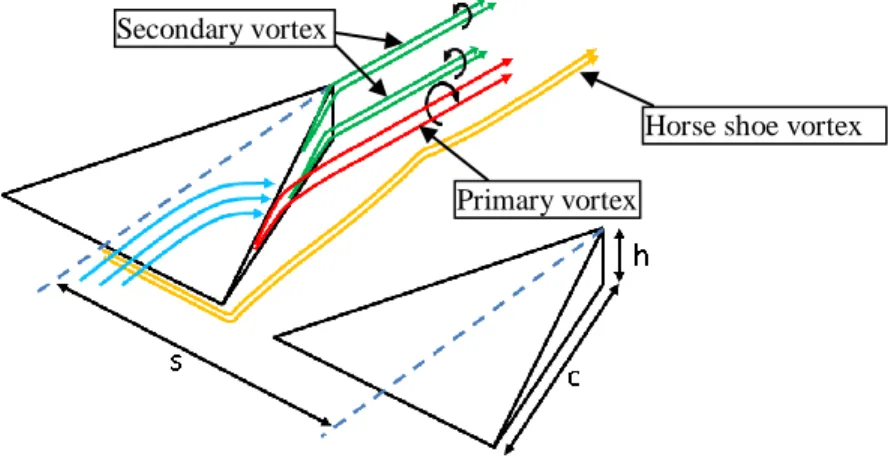
Hybrid flow control is an alternative to boundary-layer bleed. It is a combination of micro-ramp1 flow control devices and micro-jets to energize the boundary layer by transferring and inducing high-momentum flow respectively. Micro-ramps are a type of vortex generator (VG). VGs have been successfully used in the past for subsonic diffusers to avoid flow separation. Traditional VGs are typically the height of the boundary-layer thickness; however, micro-ramp heights are on the order of 25%-40% of the boundary-layer thickness. Micro-ramps generate primary counter-rotating vortices that transfer the high-momentum flow from the outer boundary layer to the flow near the wall. Even though this results in high-momentum flow in the near-wall region; it comes with the cost of low-momentum flow away from the wall. To reduce this deficit, flow is injected over the micro-ramps. Research2,3 has also shown the evidence of secondary counter-rotating vortices in line with the micro-ramp. Figure 1 shows these flow features on one-half of the micro-ramp.
Figure 1: Micro-ramp flow features schematic
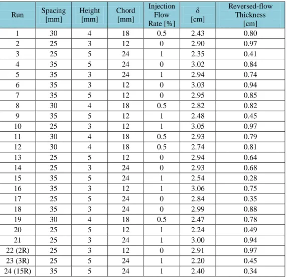
Past research efforts4,5,6 have studied only micro-ramps as the flow control device. Moreover, these were focused towards SBLI on a flat surface which is common within inlet internal flowpath. Thus, an experimental investigation of SBLIs was performed in the 15x15 cm Supersonic Wind Tunnel (SWT) at the NASA Glenn Research Center to evaluate the effectiveness of the hybrid flow control on the normal shock induced separation. To emulate a contoured fuselage surface which is common in the design of integrated inlets, a bump was used. A total of 17 hybrid flow control configurations were tested as part of the test matrix, which was developed using Design of Experiments (DOE) methods. The variables of interest were inter-ramp spacing (s), ramp height (h), ramp chord length (c), and percent of freestream mass flow injected through the injection holes (IFR). The IFR ranged from 0-1% of tunnel freestream mass flow. In addition to the 17 DOE configurations, data were also obtained for the baseline tunnel configuration, which consisted of no micro-ramps and no flow injection. To understand the flow features qualitatively, oil flow visualization was used to identify the location of shock impingement on the wall, separation size, path of the counter-rotating vortices, and corner flow effects. Improvements in the boundary-layer state will be compared in terms of the boundary-layer thickness and reversed-flow thickness. Reversed-flow thickness is defined as the separated flow within the boundary layer where the pitot pressure is less than or equal the wall static pressure.
This paper presents the results from the boundary-layer survey data as well as DOE analysis that examined the effects of the above mentioned four variables on the reversed-flow thickness and boundary-layer thickness. The DOE analysis helped to identify the dominant variables and the effects of variable interactions.
Horse shoe vortex Primary vortex
3
II. Experimental Setup
A. 15x15 cm Supersonic Wind Tunnel (SWT)
The 15x15 cm SWT, shown in Fig. 2, is a continuous flow facility in the Engine Research Building at NASA Glenn Research Center. The inflow is connected to the central air supply, which provides up to 280 kPa (40 psig) pressure at ambient temperature. The supply air is controlled by an upstream valve that adjusts the test section total pressure. The exhaust is captured by the central altitude exhaust system, which is capable of sustaining pressures less than 14 kPa (2.0 psia).
The test section, shown in Fig. 3, has a constant area of 15x15 cm (5.91x5.91 in) and configurable insert sections on each of the four walls. Immediately after the test section, the flow encounters a rearward facing step where the tunnel area expands to 23.5x23.5 cm (9.25x9.25 in).
The tunnel has an exchangeable nozzle capability that allows a range from subsonic flow up to Mach 3.0. For the purpose of this experiment, the subsonic (constant area) nozzle block was used to obtain Mach 0.67 flow at the entrance to the test section. As shown in Fig. 3, the top wall of the test section is comprised of a bump. As the flow travels past the bump it accelerates to Mach 1.3. A normal shock positioned at the aft portion of the bump effectively brought it back to subsonic speed. To position the normal shock in the test section, the tunnel was back pressured by controlling the downstream valve. The inlet total pressure was set to obtain a constant freestream Reynolds number of 13.1E6 /m (4.00E6 /ft).
Figure 2: 15x15 cm Supersonic Wind Tunnel
Figure 3: Layout of the tunnel test section with key axial locations
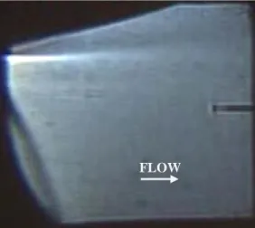
Figure 4 shows a schlieren image of the test section where the normal shock is located. The area of interest was the flow just downstream of the shock impingement on the bump. Due to the limited field of view on the schlieren
system, the exact SBLI location is not captured, but the low-momentum high shear region can be observed as the bright white streak.
Figure 4: Schlieren view of the normal shock location on the bump
The total pressure probe can also be seen in the image. The flow was probed vertically immediately after the bump, see Fig. 3 for the boundary layer survey axial location. The vertical flow measurements were made from the wall up to 3-4 cm extending into the freestream depending on the configuration. The intent was to characterize the boundary layer separation immediately downstream of the shock impingement.
B. Micro-ramps and Micro-jet Flow Injection Design
The micro-ramps were intended to reduce the shock induced separation on the aft end of the bump. For this purpose, four micro-ramps were positioned laterally, symmetric about the tunnel centerline. Figure 5 shows the micro-ramp geometry in terms of parameters s, h, and c. These parameters, along with the flow injection rate, were varied to obtain the test matrix. The micro-ramp half angle, α, was held constant at 24 degrees. Based on previous experience6, inter-ramp spacing (s) was investigated at three levels: 25, 30, and 35 mm; ramp height (h) at three levels: 3, 4, and 5 mm, and ramp chord length (c) at three levels: 12, 18, and 24 mm.
(a) (b)
Figure 5: Micro-ramp geometry parameters shown in (a) Top view and (b) Side view
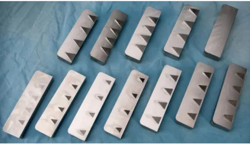
Although 11 micro-ramp configurations were fabricated, only nine were tested as part of a shorter DOE test matrix due to time constraints. Figure 6 shows the 11 micro-ramp configurations (and 1 blank) obtained using DOE where s, c, and h (Fig. 5) were varied. The micro-ramp inserts were mounted on the injection assembly (Fig. 7) which is laterally centered in the tunnel.
5
Figure 6: Micro-ramp inserts
The micro-jet flow injection was intended to reduce the momentum deficit created by the pair of counter-rotating vortices which transfers the high-momentum flow from the boundary-layer edge to near the wall. A computational fluid dynamic (CFD) analysis of 20º, 40º, and 60º injection port had shown that the 20º injection port had the most effect on the boundary-layer improvement. Thus, the 20º injection port was used for this test. Figure 7 shows the micro-ramps and injection assembly, where the injection ports are just upstream of the micro-ramps. The 20º injection ports were aligned with the micro-ramps so that the flow injection was centered over the micro-ramps. Three injection port configurations were fabricated to match the three inter-ramp spacings of 25, 30, and 35 mm. An upstream valve to the injection plenum was used to regulate the level of micro-jet injection flow ratio (IFR) which was 0%, 0.5% and 1.0% of the freestream mass flow rate.
Figure 7: Micro-ramps and micro-jets assembly
C. Instrumentation and Data Systems
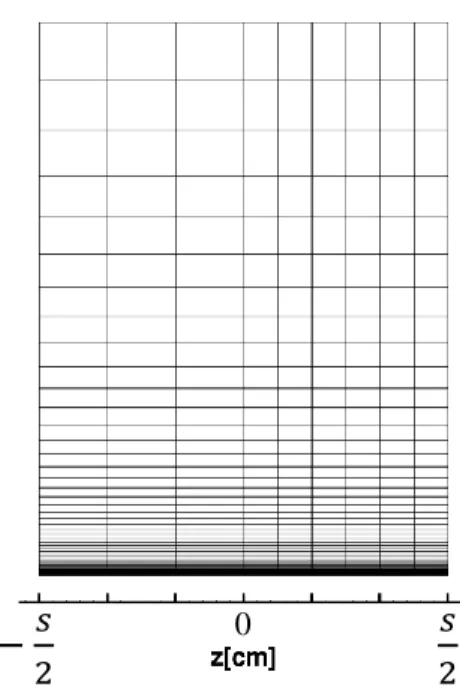
The boundary-layer profiles immediately downstream of the bump were the primary data of interest. The measurement plane was located at x ≈ 34 cm, shown by a green vertical line in Fig. 3. A total of 10 y-z profiles were obtained at selected z locations and each profile contained approximately 57 data points, shown in Fig. 8. A translating flat-tip total pressure probe was used to make these boundary-layer measurements. In addition to the probe data, 12 static pressure taps were place along the bump contour to determine the normal shock location.
Figure 8: Measurement plane
D. Oil Flow Visualization
Oil flow visualization technique was used to reveal and recognize subtle flow features like pairs of downstream moving counter-rotating vortices generated by each micro-ramp, spanwise normal shock impingement, corner flow separation, and SBLI. Flow visualization, although primarily qualitative, is a supplementary tool which helps understand flow physics and the effects of the hybrid flow control.
Green and orange fluorescent pigment was mixed with oil to create an oil-pigment mixture. This was applied to the bump surface in a three stripe pattern, shown in Fig. 9. For the purpose of flow visualization, the tunnel was quickly brought to run conditions and a camera was used to monitor the bump surface and determine if the oil-pigment mixture had reached steady state, i.e. the flow patterns in Fig. 9 had developed and oil-oil-pigment mixture movement on the bump surface was minimal. A black light was used to enhance the view of the bump surface. When the flow pattern appeared to have fully established, the tunnel was quickly shut down and surface oil flow images were obtained.
Figure 9 shows an example of this flow visualization technique. The discussion of the flow features will follow in the Results section.
Figure 9: Flow visualization example
0
7
III. Design of Experiments
Central Composite and Full Factorial Design of Experiments (DOE) methods were initially picked for the evaluation. However, based on previous experience2, the Full Factorial DOE analysis was picked for the purpose of this work. The boundary-layer thickness and reversed-flow thickness were chosen as the response variables for the DOE analysis. A prediction model obtained from a DOE analysis could be used to estimate the effects of factor variables on the response variables.
A full factorial design allows for estimation of the first-order effects and first-order interactions. The design will never saturate as there are 17 configurations tested and only 11 coefficients to calculate assuming all first-order effects and interactions are statistically meaningful. The design also allows for five center point (replicating the one center point four times). In addition to the center point, three runs (2, 3, and 15) were replicated. Thus, a total of 24 cases comprised in the DOE test matrix. This design has six degrees of freedom (6 runs) to determine quality of fit and seven degrees of freedom (7 runs) to determine error of the model. The remaining 11 runs will be used to estimate the 11 coefficients in Eq. 1.
A response equation for boundary-layer thickness would be of the form:
(1) The actual terms and coefficients of the above equation will depend on the significance of the first-order effect and the interactions. Just like other statistical tools, success of this DOE analysis depended on a careful and systematic data collection approach to avoid introduction of random and user errors.
Table 1: Full Factorial test matrix
Run Spacing [mm] Height [mm] Chord [mm] Injection Flow Ratio [%] 1 30 4 18 0.5 2 25 3 12 0 3 25 5 24 1 4 35 5 24 0 5 35 3 24 1 6 35 3 12 0 7 35 5 12 0 8 30 4 18 0.5 9 35 5 12 1 10 25 3 12 1 11 30 4 18 0.5 12 30 4 18 0.5 13 25 5 12 0 14 25 3 24 0 15 35 5 24 1 16 35 3 12 1 17 25 5 24 0 18 35 3 24 0 19 30 4 18 0.5 20 25 5 12 1 21 25 3 24 1 22 (2R) 25 3 12 0 23 (3R) 25 5 24 1 24 (15R) 35 5 24 1
IV. Results
A. Baseline Case
A baseline configuration (no hybrid flow control) was tested to characterize the flow with a normal shock in the absence of flow control. Boundary-layer total pressure profiles were obtained using the translating probe at various spanwise locations. This total pressure data was used to calculate the velocity. The eight digit code, 00-00-00-00, is a unique identifier for the baseline case where flow control was not used. Each two digits represents flow control parameters (s, h, c, and IFR). For the flow injection cases, a period should be interpreted between the two digits. A value of “05” means 0.5 and “10” means 1.0. For example, Run 1 in Table 1 can be identified as 30-04-18-05.
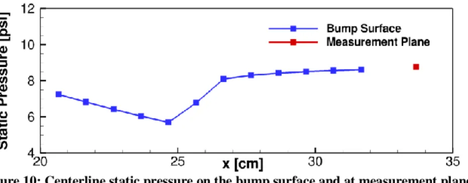
Immediately downstream of the normal shock impingement, the flow separated. The pressure measurements made by the pitot pressure probe were lower than the static pressure measured at the wall surface. Although the difference in the pressure was within the measurement uncertainty, the lower pressures measured by the probe were indicative of a large separation. The bump centerline static pressure in Fig. 10 shows the increase in static pressure across the normal shock. However, the static pressures were nearly constant from axial location of x ≈ 27 to 34 cm, which shows a large separation exists at the aft end of the bump.
Figure 10: Centerline static pressure on the bump surface and at measurement plane
The velocity within the separated flow was assumed to be equal zero where pitot pressure was less than or equal the wall static pressure. This was evident from the vertical velocity profile, ulocal/u∞ = 0, close to the wall in the measurement plane (Fig. 11). The velocity profiles at various z (span) locations appear to vary with subtle differences.
Figure 11: Baseline velocity profiles (no flow control)
Tunnel centerline
9
Table 2 shows the boundary-layer thickness and the reversed-flow thickness at each spanwise location. The boundary-layer thickness was calculated assuming the height at which uδ = 0.99u∞ occurred and the reversed-flow thickness is equal to the largest y-value where the total pressure measured by the pitot probe was equal to the local static pressure (ulocal/u∞ = 0). In the absence of an automatic pressure regulator, the back pressure in the tunnel was manually adjusted to keep the normal shock position constant on the bump. Although the back pressure was carefully adjusted and the P∞/Pback was relatively constant, the pressure ratio varied by ±0.01 within a boundary-layer profile. As the probe translated through the inner boundary boundary-layer, finer pressure adjustments were required to keep the normal shock position constant, however due to the mechanical limitation on the valve this was not possible.
The span-averaged boundary-layer thickness was 2.88 cm and the reversed-flow thickness was 0.97 cm for the baseline case. Figure 12 shows a flow visualization image of the baseline case. The SBLI is evident and most of the oil-pigment mixture is collected just after the shock. The orange oil-pigment mixture from the side wall flows on the bump surface which shows the evidence of corner flow separation.
Table 2: Spanwise boundary-layer parameters for Baseline case
z [cm] δ [cm] Reversed-flow Thickness [cm] -1.5 2.94 0.90 -1 3.01 1.00 -0.5 2.96 1.00 0 2.96 1.00 0.25 2.94 1.00 0.5 2.74 1.00 0.75 2.70 0.95 1 2.80 1.00 1.25 2.88 0.95 1.5 2.92 0.90 Span-average 2.88 0.97
Figure 12: Flow visualization for Baseline case
FLOW
Normal shock
Orange pigment from side wall
x~25 cm x~33.5 cm
x~16 cm
B. Hybrid Flow Control Configurations
The velocity profiles at z = -s/2 and s/2 cm were obtained in line with the micro-ramps, which is also referred to as the upwash region while the velocity profile at z = 0 was obtained in the center of two micro-ramps at the tunnel centerline, which is also referred to as the downwash region. A summary of span-averaged boundary-layer parameters for various configurations is listed in Table 3. From here on, the discussion will use span-averaged parameters, unless mentioned otherwise.
Table 3: Span-averaged boundary-layer parameters for all flow control cases
Run Spacing [mm] Height [mm] Chord [mm] Injection Flow Rate [%] δ [cm] Reversed-flow Thickness [cm] 1 30 4 18 0.5 2.43 0.80 2 25 3 12 0 2.90 0.97 3 25 5 24 1 2.35 0.41 4 35 5 24 0 3.02 0.84 5 35 3 24 1 2.94 0.74 6 35 3 12 0 3.03 0.94 7 35 5 12 0 2.95 0.85 8 30 4 18 0.5 2.82 0.82 9 35 5 12 1 2.48 0.45 10 25 3 12 1 3.05 0.97 11 30 4 18 0.5 2.93 0.79 12 30 4 18 0.5 2.74 0.81 13 25 5 12 0 2.94 0.64 14 25 3 24 0 2.93 0.68 15 35 5 24 1 2.54 0.28 16 35 3 12 1 3.06 0.75 17 25 5 24 0 2.84 0.35 18 35 3 24 0 2.99 0.88 19 30 4 18 0.5 2.47 0.78 20 25 5 12 1 2.24 0.49 21 25 3 24 1 3.00 0.94 22 (2R) 25 3 12 0 2.91 0.97 23 (3R) 25 5 24 1 2.20 0.45 24 (15R) 35 5 24 1 2.40 0.34
1. Micro-jet Injection Flow Rate (IFR) effect
As discussed earlier, micro-ramps generate a pair of counter-rotating vortices that brings the high-momentum flow at the edge of the boundary layer to the wall. However, the process creates a momentum deficit at the edge of the boundary layer as a result of flow transfer. This is illustrated in IFR = 0% (35-05-24-00, Run 4) shown in Fig. 13 and IFR = 0% (25-05-24-00, Run 17) in Fig. 14. Figure 13 shows the effect of IFR at s = 35 mm and Fig. 14 at s = 25 mm.
11
Figure 13: Injection flow rate effect on the boundary-layer thickness at s = 35 mm
In the absence of flow injection, the region of momentum deficit can be clearly seen in the upwash profile in the region of ulocal/u∞ = 0.85-0.95 for Fig. 13. Also, there was no improvement in the boundary-layer thickness and reversed-flow thickness in the downwash profile. The effect of counter-rotating vortices does not extend to the downwash region without flow injection for s = 35 mm. The span-averaged boundary-layer thickness improved from 3.02 cm to 2.40 cm as the flow injection was turned on. Deeper flow penetration in the upwash region for IFR = 1% also confirms the influence of secondary counter-rotating vortices.
Figure 14: Injection flow rate effect on the boundary-layer thickness at s = 25 mm
Upwash Downwash Back-pressure adjustment Upwash Downwash Back-pressure adjustment Momentum deficit Momentum deficit
A prominent momentum deficit can be seen in the upwash profile where IFR = 0% in Fig. 14. This momentum deficit is filled when flow injection is turned on for Run 3R (25-05-24-10), however a negative effect was observed in the downwash region supported by an increase in the reversed-flow thickness. In contrast with Run 4 (35-05-24-00), Run 17 (25-05-24-(35-05-24-00), where micro-ramps are placed 25 mm apart, did produce a flow improvement in the downwash region. This is due to the fact that short inter-ramp spacing allows the effect of counter-rotating vortices to extend in the downwash region and flow injection is not needed to propagate that effect. The upwash and downwash profiles are relatively identical for IFR = 0%, except the deficit region; this flow uniformity is favorable for an engine aerodynamic interface plane (AIP). The span-averaged boundary-layer thickness was improved from 2.84 cm for IFR = 0% to 2.20 cm for IFR = 1% as the flow injection was turned on.
The results show that flow injection will be a strong first-order effect in DOE analysis with possible significant interaction with inter-ramp spacing.
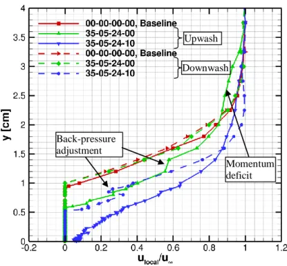
2. Inter-ramp spacing effect
Table 3 shows that the best improvement in the boundary-layer thickness, was obtained for the s = 25 mm (25-05-24-10, Run 23) which means the inter-ramp spacing was the smallest of the three tested. Figure 15 shows the effectiveness of micro-ramps as well as micro-ramps as part of the hybrid flow control system with respect to inter-ramp spacing in the upwash and downwash regions of a micro-inter-ramp. A comparison of two cases, s = 25 mm and 35 mm is presented with the baseline case. The ramp height, ramp chord length, and flow injection were constant for this comparison. The plotted upwash profile is directly in line with a micro-ramp (located at z=–s/2) while the downwash profile is obtained at the tunnel centerline (z=0).
The inter-ramp spacing of 25 mm is the best performing micro-ramp with a reduction in span-averaged boundary-layer thickness of 0.68 cm. Although s = 35 mm (35-05-24-10, Run 24) did not produce the lowest boundary-layer thickness, the reversed-flow thickness was lower than s = 25 mm configuration. Thus, increasing the inter-ramp spacing had a positive effect on the reversed-flow thickness. The counter-rotating primary vortices induced flow penetrated deeper in the boundary layer and eliminated the reversed flow for s = 35 mm in the upwash region, however the downwash region remained unchanged. Improvement in the upwash region was likely influenced by secondary rotating vortices as well. Placing micro-ramps 35 mm apart allowed the counter-rotating vortices to develop independently and not negatively impact the neighboring pair.
Figure 15: Inter-ramp spacing effect on the boundary-layer thickness
Figure 15 also highlights an important difference between the upwash and downwash regions of a micro-ramp flow field. The profiles obtained in the upwash region are fuller as the high-momentum flow from the
boundary-Upwash Downwash
Back-pressure adjustment
13
layer edge is transferred to the wall. However, the boundary layer was thicker in the upwash region. The downwash profile is shallow and there is still evidence of the low-momentum reversed flow close to the wall, although, the downwash region has a thinner boundary layer. The results suggest that inter-ramp spacing will be a strong first-order effect with possible coupled interactions.
The fluctuation in the downwash profile at ulocal/u∞ = 0.25 is an artifact of manual adjustment made to the back pressure to maintain a constant normal shock position. As discussed earlier, this was unavoidable due to mechanical limitations.
3. Ramp height effect
Figure 16 shows a comparison of h = 3 mm (35-03-24-10, Run 5) and h = 5 mm (35-05-24-10, Run 24) with the baseline case. Inter-ramp spacing, ramp chord length, and IFR were constant for this comparison.
The micro-ramps with h = 3 mm generate a pair of counter-rotating vortices that do not cause flow penetration to the wall; as a result the layer of reverse flow still exists. In contrast, the micro-ramps with h = 5 mm have deeper penetration and eliminate the layer of reverse flow. The boundary-layer thickness for h = 3 mm was 2.94 cm while that of h = 5 mm was 2.40 cm, which clearly shows the benefit of a larger micro-ramp height.
The upwash profile for h = 3 mm shows some improvement in the boundary layer however, the downwash profile shows insignificant improvement when compared to the baseline case. This is likely due to the fact that the low ramp height is producing small and weak counter-rotating vortices which do not have effect on flow improvement in the downwash region. In contrast, h = 5 mm micro-ramps produced the largest flow improvement in the upwash and downwash region. Ramp height will also have significant first-order effect with interactions.
Figure 16: Ramp height effect on the boundary-layer thickness
4. Ramp chord length effect
The upwash and downwash profiles of c = 12 mm (25-05-12-10, Run 20) and c = 24 mm (25-05-24-10, Run 23) are compared with that of baseline case in Fig 17. Inter-ramp spacing, ramp height, and IFR were constant for this comparison. Although the profiles show a flow improvement, the effect of change in chord length is insignificant. The c = 24 mm micro-ramps have a deeper flow penetration than the c = 12 mm micro-ramps; however, neither eliminates the layer of reversed flow that exists at the wall. The results showed that the chord length plays a small role in the shape and size of the counter-rotating vortices.
Upwash Downwash
Back-pressure adjustment
In Fig. 17, the upwash region has a fuller profile while the downwash region has a shallow profile. The boundary-layer thickness and reversed-flow thickness were 2.24 cm and 0.486 cm respectively for c = 12 mm and 2.20 cm and 0.446 cm for c = 24 mm respectively.
Figure 17: Ramp chord length effect on the boundary-layer thickness
C. Reversed-flow Thickness Analysis
For this highly separated flow, the thickness of the region of reversed flow was used as a response parameter. The reversed-flow thickness is equal to the largest y-value where the total pressure measured by the pitot probe was equal to the local static pressure (ulocal/u∞ = 0). The following sub-section explores the effects of two factor interactions.
The counter-rotating vortices produced by the micro-ramps cause a spanwise variation in boundary-layer properties. Figure 18 shows spanwise profiles of reversed-flow thickness for two VG configurations. For both profiles, the largest reversed-flow thickness occurred at z = 0 cm, in the downwash region. The thinnest region of the boundary layer is directly downstream of the tip of the ramps. The amount of variation in the spanwise direction differed significantly between configurations, with cases varying as much as 0.575 cm to as little as 0.075 cm in reversed-flow thickness across the span. Run 15 (35-05-24-10) was the only one that segmented the separation by eliminating the separation at z = ±1.5 cm, the upwash region.
Figure 18: Spanwise variation in reversed-flow thickness for two VG configurations
Upwash Downwash
Back-pressure adjustment
15
Not including the DOE center point (30-4-18-05), 16 VG configurations were tested. Span-averaged values of reversed-flow thickness were calculated for each case. Fixing any two of the factor variables at constant levels (e.g. h = 3 mm, IFR = 0.0 %) reduces the full test matrix to a set consisting of four cases. Because the test matrix was laid out orthogonally, this set of cases has balanced levels of the remaining factor variables (e.g. two with c = 12 mm, two with c = 24 mm, and two with s = 25 mm, two with s = 35 mm). For each set, the span-averaged reversed-flow thicknesses of the four cases were averaged to get a set average. This process is illustrated in Table 4 using the device height, h, and the injection flow ratio, IFR, as the fixed variables.
Table 4: Example of finding set averages for the h-IFR interaction.
Run s, mm h, mm c, mm IFR, % Span-Averaged Reversed-flow Thickness, cm 2 25 3 12 0 0.97 6 35 3 12 0 0.94 14 25 3 24 0 0.68 18 35 3 24 0 0.88 Set Average: 0.87 4 35 5 24 0 0.84 7 35 5 12 0 0.85 13 25 5 12 0 0.64 17 25 5 24 0 0.35 Set Average: 0.67 5 35 3 24 1 0.74 10 25 3 12 1 0.97 16 35 3 12 1 0.75 21 25 3 24 1 0.94 Set Average: 0.85 3 25 5 24 1 0.43 9 35 5 12 1 0.45 15 35 5 24 1 0.31 20 25 5 12 1 0.49 Set Average: 0.42
The graphs in Fig. 19 show interactions of the factor variables. One factor variable is represented on the x-axis, and the other is indicated by color. The solid lines in Fig. 19 show the values of the set average, whereas the dashed lines correspond to the maximum and minimum values within the set.
(a) (b)
(c) (d)
Figure 19: Factor variable interaction effects on reversed-flow thickness. Solid lines indicate set average values, and dashed lines indicate the maximum and minimum recorded values within the set. (a) h-IFR interaction, (b) h-s
interaction, (c) IFR-s interaction, and (d) h-c interaction
Figure 19a shows how height and injection flow rate interact to influence the reversed-flow thickness. For the small micro-ramp height, both the range and the average values of reversed-flow thickness are not influenced by IFR. For the large micro-ramp height, injection has a strong positive influence on reversed-flow thickness: the average value of reversed-flow thickness is significantly lower, and the range of values is reduced. It is interesting to note, though, that the minimum value attained for each level of IFR is similar.
The height-spacing interaction is shown in Fig. 19b. Similarly to the previous case, spacing has little influence for the ramps with h = 3 mm. For the ramps with h = 5 mm, the average value of reversed-flow thickness is lower for devices spaced more closely together.
Taking Fig. 19a and 19b together, it might be hypothesized that the optimal hybrid flow control configuration would be devices with a large height, 1.0 % injection, and spaced closely together. However, Fig. 19c contradicts this assumption. Looking at the interaction between IFR and spacing shows that for devices spaced closely together, increasing IFR has a small, and slightly negative, effect. For devices spaced farther apart, injection has a positive effect.
The height-chord length interaction is less complicated. For both device heights, the larger chord length performs better, as seen in Fig. 19d.
There were two hybrid flow control configurations that were very effective in reducing the reversed-flow thickness: large ramps (h = 5 mm, c = 24 mm) spaced closely together without injection, and large ramps spaced farther apart with 1.0% IFR. The configuration without injection would require less complex hardware, and also generated a more uniform spanwise profile than the case with injection. The case with injection was the only one for which an attached profile was measured in any spanwise plane and the small range between the minimum and
17
maximum levels of reversed-flow thickness seen for h = 5 mm, IFR = 1.0 % in Fig. 19a indicated robustness in the design.
D. Oil Flow Visualization
Even though exhaustive image processing was not employed, a relatively simple flow visualization technique which uses a layer of oil-pigment mixture on the bump surface illuminated by a black light was utilized. This technique provides a great deal of insight in the flow physics of hybrid flow control. It was an inexpensive tool to supplement discrete data and capture flow physics where the bump surface was not instrumented. A total of five cases were picked for flow visualization which included the baseline case.
Figure 20 presents a comparison of two cases, Run 4 with and Run 15 without flow injection. The cases were selected because they shed light on the distinctive features of hybrid flow control.
The trailing edge of the micro-ramps shows a collection of oil-pigment mixture which could be attributed to a pocket of separated flow as the pair of counter-rotating vortices detach and moves downstream. Shocks also appear to be coming off of each micro-ramp which coincide in the downwash region. Shocks only appear in the cases with flow injection and can be seen in Fig. 20b. As the streamlines pass through the shocks they seem to linger and continue on. Figure 21 shows a close-up of the center two micro-ramps where the miniature flow separation on the micro-ramp trailing edge and shocks are clearly seen.
(a) Run 4 – 35-05-24-00
(b) Run 15 – 35-05-24-10
Figure 20: Flow visualization comparison
The path of the downstream moving secondary vortex pair is distinct and wide in Fig. 20b while it is faint and narrow in 20a which shows the effect of flow injection on the vortices development. The vertical accumulation of
FLOW
FLOW
Corner flow separation Break in flow separation
Normal shock Secondary vortices path Horseshoe vortex Secondary vortices path
oil-pigment mixture denoting the normal shock location seems to have moved downstream for the case where the flow injection is on. The break in the flow separation can also be seen in-line with the micro-ramps or the upwash region in Fig. 20b. This is in contrast to the downwash region where the flow separation is intact suggesting the vortices do not induce flow to penetrate the boundary layer. Figure 20 also show the separated corner flow moving away from the side wall in a swirl pattern. The pitot pressure measurement plane did not extend this far spanwise, thus the magnitude of separation was unknown. Such corner separation was absent in the baseline case. Figure 20a reveals that the corner separation is weaker than in Fig. 20b which implies that the introduction of micro-ramps possibly triggered the corner separation and flow injection increased the magnitude of it. It is likely that the corner flow separation was a tunnel characteristic.
Figure 21: Micro-ramps close-up (Run 15)
E. DOE Analysis
The boundary-layer thickness (δ) and reversed-flow thickness are not limited to the first-order effects of inter-ramp spacing, inter-ramp height and chord, and flow injection. The first-order effects demonstrated in the previous sub-sections play an important role in obtaining a valid response model, however for this work it was found that second-order effects as well as two- and three-level interactions play a decisive role in estimation of a prediction model.
Based on previous successful use2, it was decided that the first-order effects and two-level interactions would be sufficient to obtain a response model. Thus, a test matrix, Table 1, was designed with this assumption. A post-test DOE analysis of the experimental data showed that the full factorial DOE method was inadequate to predict the response model of the form showed in Equation 1. Further, investigation showed that the experimental data had a significant curvature (i.e. parabolic) which means second-order effects and two- and three-level interaction terms were needed to be part of the prediction model. This can be attributed to the fact that the current experimental setup comprised of a normal shock impinging on a bump surface which results in a massively separated flow. By contrast, the previous work was done to investigate micro-ramp effectiveness on flow separation caused by an oblique shock. An additional parameter, flow injection is also being studied which makes present experimental work much more complex than the previous.
In order to obtain a semi-useful prediction model, the experimental data was analyzed with a custom, central composite type, DOE method. Although, the test matrix was not designed to estimate higher order effects, the effort gave an interesting insight into the experimental data which, while unsuccessful, showed a strong need for the central composite DOE method which considers first- and second-order effect along with two- and three-level interactions.
Currently, plans are made for a second entry into 15x15 cm SWT to finish the required test runs which will allow the prediction of δ and reversed-flow thickness.
Streamlines passing the shock
19
V. Conclusions
Hybrid flow control configurations were tested in the 15x15 cm SWT at NASA GRC. A full factorial DOE method was used to design the test matrix to investigate four variables, inter-ramp spacing, ramp height and chord length, and flow injection. The results showed that a full factorial DOE method, which takes first-order effects and two-level interactions into account, is inadequate to predict a response model for boundary-layer thickness (δ) and reversed-flow thickness. The presence of a normal shock and resulting separation requires higher order effects and interactions for accurate response estimation. Central composite DOE method would be more suitable for the present work as it also considers statistically significant second-order effects and two- and three-level interactions.
Nonetheless, experimental data was analyzed and first-order effects and two-level interactions were investigated individually. The inter-ramp spacing, ramp height, and IFR were found to have a significant first-order effect and interactions. The ramp chord length has a subtle first-order effect and interactions.
Inter-ramp spacing of 35 mm and ramp height of 5 mm produce a stronger and larger pair of counter-rotating vortices which was able to induce flow that penetrate the boundary layer and energize the near wall region. In general, these cases produced a lower value of reversed-flow thickness, which is a more suitable measure of boundary-layer health than boundary-layer thickness in such massively separated flow. Smallest values of inter-ramp spacing and inter-ramp height produce a weaker and smaller pair of counter-rotating vortices which was unable to induce high-momentum flow to the wall. This resulted in a layer of reversed flow close to the wall.
The micro-jet flow injection effect was visibly obvious as it filled the momentum deficit created by the counter-rotating vortices and energized them. IFR of 1% showed the most improvement when combined with the largest micro-ramps. Results also showed that the two and three-level interactions were significant along with the first- and second-order effects.
Oil flow visualization proved to be a quick and economic tool that could be used for evaluation of hybrid flow control. It was instrumental in identifying the corner flow effect which became increasingly significant as the flow control was turned on. It was effective at emphasizing obscure flow features which would go unnoticed in the absence of costly instrumentation.
Although additional test runs are required to obtain a meaningful response model of boundary-layer thickness and reversed-flow thickness, the data showed that the hybrid flow control is a promising approach to make flow improvement in shock induced flow separation.
Acknowledgements
The authors would like to acknowledge the support of engineering staff at the 15x15 cm SWT at NASA Glenn Research Center. The Supersonics Project of the NASA Fundamental Aeronautics Program supported this work.
References
1
Anderson, B. H., Tinapple, J., Surber, L., “Optimal Control of Shock Wave Turbulent Boundary Layer Interactions using Micro-Array Actuation,” AIAA-2006-3197, 2006.
2
Babinsky, H., Li, Y., Pitt Ford C. W., “Microramp Control of Supersonic Oblique Shock-Wave/Boundary-Layer Interactions,” AIAA Journal, Vol. 47, No. 3, 2009.
3
Galbraith, M. C., Orkwis, P. D., Benek, J. A., “Multi-Row Micro-Ramp Actuators for Shock Wave Boundary-Layer Interaction Control,” AIAA Paper 2009-321, 2009.
4
Lee, S., Goettke, M. K., Loth, E., Tinapple, J., Benek, J., “Microramps Upstream of an Oblique-Shock/Boundary-Layer Interaction,” AIAA Journal, Vol. 48, No. 1, 2010.
5
Herges, T., Kroeker, E., Elliott, G., Dutton, C., “Micro-Ramp Flow Control of Normal Shock/Boundary-Layer Interactions,” AIAA Paper 2009-920, 2009.
6
Hirt, S. M., Anderson, B. H., “Experimental Investigation of the Application of Microramp Flow Control to an Oblique Shock Interaction,” AIAA-2009-919, 2009.