MASTER'S THESIS. Using Particle-Swarm Optimization for Antenna Design

(1)

M A S T E R ' S T H E S I S

Using Particle-Swarm Optimization

for Antenna Design

Magnus Olofsson

Luleå University of Technology MSc Programmes in Engineering

Department of Computer Science and Electrical Engineering EISLAB

(2)

Using Particle-Swarm Optimization for

Antenna Design

Magnus Olofsson

Lule˚

a University of Technology

Dept. of Computer Science and Electrical Engineering

EISLAB

(3)

(4)

A

BSTRACT

From a historical perspective, electromagnetic modelling and its techniques of optimiza-tion are relatively new to the academic community. Their existence has facilitated the development of complex electromagnetic structures, and provides invaluable aid when designing electronic products that face strict radiation legislation. This thesis provides an introduction to electromagnetic modelling using the Partial element equivalent cir-cuit (PEEC) method, and an in-depth description and evaluation of the technique of particle-swarm optimization.

PEEC is a current research topic at the Embedded Internet Systems Laboratory (EIS-LAB). This approach describes electromagnetic models and couplings by equivalent cir-cuits. It arises from inductance calculations and allows for inclusion of lumped elements describing voltage sources, resistances, inductances, and capacitors. As a direct result of the research, a local electromagnetic solver is available.

The main objective is to merge the existing EISLAB solver with the particle-swarm algorithm, for optimizing various electromagnetic structures. A technique for calculating the radiated field from the models is also discussed and used for the purpose of optimizing a dipole array.

Particle-swarm optimization was developed in 1995 and models the movement and intelligence of swarms. Behind the algorithm are a social psychologist and an electrical engineer, who developed the optimizer inspired by nature. The technique has proven suc-cessful for many electromagnetic problems and is a robust and stochastic search method. The optimization algorithm alters the input file to the PEEC solver, thus affecting the physical description of the electromagnetic structures, and evaluates the result that is returned from the solver.

The particle-swarm algorithm worked well on several problems. It was used for opti-mizing mathematical functions and electromagnetic problems. The optimized antennas were determined to have desired resonant frequencies, high gain, and low weight and return losses. The patch antennas turned out to be troublesome to handle, thus some improvements such as inclusion of ground planes, are discussed.

(5)

(6)

P

REFACE

Finding a thesis proposal that suggested high academic level, involving complex opti-mization of electromagnetic problems, triggered a desire to carry out my Master’s thesis at the Embedded Internet Systems Laboratory, Lule˚a University of Technology.

The work surrounding the thesis puts optimization of electromagnetic problems in a new light for me. I expect that some time still remains before a generic easy-to-use electromagnetic solver exists on the market, especially with a built-in optimizer. Despite the debate whether there really exists a need for such a solver, I hope that my work will be a contribution in taking some local research projects toward optimization.

I take pleasure here in thanking Dr. Jonas Ekman, who has been very helpful and supportive. Additional gratitude goes to David and Krister who contributed to the improvement of the binary implementation of the optimization algorithm.

Magnus Olofsson

(7)

(8)

C

ONTENTS

Chapter 1: Introduction 1

Chapter 2: Introduction to electromagnetic modelling using PEEC 3

2.1 Background . . . 3

2.2 Introduction to PEEC . . . 5

2.3 Derivation of basic PEEC theory . . . 5

2.4 EISLAB’s PEEC solvers . . . 9

Chapter 3: Particle-swarm optimization 11 3.1 Background . . . 11

3.2 Genetic algorithms . . . 11

3.3 Theory . . . 12

3.4 Discrete binary representation . . . 16

Chapter 4: Electromagnetic field and antenna parameters 19 4.1 The spherical coordinate system . . . 19

4.2 Electromagnetic field from a Hertzian dipole . . . 20

4.3 Antenna parameters . . . 21

4.4 Verification of method . . . 23

Chapter 5: Implementation 25 5.1 Building blocks . . . 25

5.2 Optimization of a known function . . . 27

Chapter 6: Results 31 6.1 Antenna optimization . . . 31

Chapter 7: Conclusions and further work 37 7.1 Conclusions . . . 37

7.2 Further work . . . 37

(9)

(10)

C

HAPTER

1

Introduction

Electromagnetic interference (EMI) and electromagnetic compatibility (EMC) play a very important role in the society of today. While hardware overall decreases in size as frequencies increase, a major part of the electrical systems starts to act as radiating and receiving antennas.

Traditionally, SPICE and its counterparts have been used to model the electrical behav-ior of the systems, without the consideration of electromagnetic couplings. To estimate the latter, cumbersome manufacturing of experimental models based on experience and rules of thumb preceded measurements in shielded chambers. Since the manufacturer of incompatible devices may suffer from large fines due to the strict EMC regulations [1], the use of electromagnetic modelling and its techniques of optimization are important tools for avoiding post-production measures. The need for experimental models, is likely to decrease or be eliminated, thus saving significant amounts of time and money.

At EISLAB, the motivation for using PEEC is mainly its use of equivalent circuits. This technique is used for modelling of various physical problems, such as mechanical, thermodynamic, and ultrasonic models. The desire is to handle all types of problems as one model in one solver.

This thesis is the first step of the far-reaching objective to incorporate an optimization algorithm in EISLAB’s PEEC solver.

(11)

(12)

C

HAPTER

2

Introduction to

electromagnetic modelling

using PEEC

2.1

Background

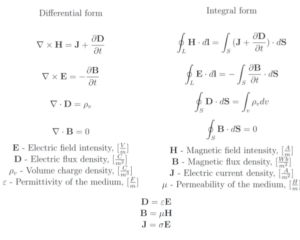
Maxwell’s equations form the backbone of electromagnetic theory. James Clerk Maxwell (1831 - 1879) was a Scottish mathematical physicist who reduced the empirical and theoretical knowledge of electricity and magnetism into a set of equations. Maxwell realized that only four1_{, at that time existing, laws are needed to completely describe}

electromagnetic field interaction with medium and source mechanisms. From [2],

I S E·dS= q ε0 (2.1) I S B·dS = 0 (2.2) Z L E·dl=− Z S ∂B ∂t ·dS (2.3) Z L B·dl=µ0(I+ε0 Z S ∂E ∂t ·dS). (2.4)

Eq. (2.1) together with (2.2) are referred to as Gauss’ law or Gauss’ law for the electric and magnetic field, respectively. The significance of the first law is that the total electric 1_{To fully constitute the basic framework of the electromagnetic theory the Lorentz force needs to be}

considered.

(13)

Table 1: The complete set of Maxwell’s equations Differential form ∇ ×H=J+ ∂D ∂t ∇ ×E=−∂B ∂t ∇ ·D=ρv ∇ ·B= 0

E - Electric field intensity, [V m]

D - Electric flux density, [ C m2]

ρv - Volume charge density, [_mC3]

ε - Permittivity of the medium, [F m] Integral form I L H·dl= Z S (J+ ∂D ∂t )·dS I L E·dl=− Z S ∂B ∂t ·dS I S D·dS= Z v ρvdv I S B·dS= 0

H - Magnetic field intensity, [A m]

B - Magnetic flux density, [W b m2]

J - Electric current density, [ A m2]

µ- Permeability of the medium, [H m]

D =εE

B =µH

J =σE

flux through an arbitrary closed surface is proportional to the total net charge inside the surface. The second law states that the magnetic flux through a closed surface is always zero, meaning that there exist no magnetic monopoles. This is quite intuitive since the lines of force of the magnetic field are always closed.

The third of Maxwell’s equations, (2.3), is called the Faraday-Henry law and relates a time-varying magnetic field with an induced electromotive force. Eq. (2.4) is called the Ampère-Maxwell law. Ampère’s law relates the magnetic circulation to a current in a conductor and was modified in 1873 by Maxwell. The second term on the right hand side will be zero if the flux of the electric field does not vary with time, as in Ampère’s approach. The modification is a direct consequence of the principal of conservation of energy, and led Maxwell to his prediction of the existence of electromagnetic waves.

By using Gauss’ divergence theorem, Maxwell’s equations also take on a differential form. This form is desirable when dealing with volume integration. Table 1 shows the complete set of Maxwell’s equations and also includes three medium-dependent equations. Index 0 of µand ε of (2.1) and (2.4) indicates that the medium is vacuum. Throughout this thesis no magnetic medium will be considered, thus makingµ=µ0.

(14)

2.2. Introduction to PEEC 5

2.2

Introduction to PEEC

The PEEC method [3, 4, 5] arises from inductance calculations by Albert E. Ruehli at IBM T.J. Watson Research Center in 1970. The PEEC approach has been proven suc-cessful for the modelling of electromagnetic problems and allows for inclusion of lumped elements describing voltage sources, resistances, inductances and capacitors. This fea-ture makes it, among other things, very suitable for modelling of printed circuit boards (PCBs) and since no discretization of the air is needed, large structures can be modelled without immense inherited computational complexity.

2.3

Derivation of basic PEEC theory

The scalar electrical potential, φ, is related to the electric field intensity according to (2.5). In analogy there exists a vector magnetic potential, A, which is defined by (2.6).

E=−∇φ (2.5)

∇ ×A=B (2.6)

If ∇ ·A= 0 is imposed, the vector magnetic potential is given by [6]

A= Z v µJ 4πrdist dv, (2.7)

whereJ is a current density vector and rdist is the distance between the observer and the source. The potential from a charge distribution is given by [6]

φ= Z v q 4πεrdist dv, (2.8)

whereqis the charge density andrdist is the distance between the observer and the charge distribution.

These expressions are presented under quasi-static conditions, meaning that the elec-tromagnetic waves travel at an infinite speed. Since the waves do propagate at a finite speed, the expressions must be dependent on time. This is indicated below by intro-ducing t. The significance of rdist in (2.7) and (2.8) stays the same, but since there is a strong need to handle more than one element, r and r0

k are introduced. The vector r points from the origin to the observer, and each r0

k is a vector pointing from the k:th source to the observer. The time delay is defined as |r−r0

k|/c, where c is the speed of light in vacuum, or approximately 3·108 _{m/s. In the frequency domain, the propagation}

delay results in a phase shift equal to ω|r−r0 k|/c.

(15)

2.3.1

Derivation of the electric field integral equation (EFIE)

The contents of the following subsections mainly originate from [7]. A basic understand-ing is important for realizunderstand-ing the complexity of large 3D structures, the limitations of the numerical models, and for the postprocessing explained in Chapter 4.

The starting point is to consider the total electric field,ET₍_r_{, t}_{) in (2.9), to be the sum} of a potential applied external electric field,Ei₍_r_{, t}_{), and a scattered field,}_ES₍_r_{, t}_).

ET₍_r_{, t}_{) =} _Ei₍_r_{, t}_{) +}_ES₍_r_{, t}₎ _(2.9)

The latter is considered to be the sum of the negative time derivative of the magnetic vector potential, and the negative gradient of the electric scalar potential, where

ET₍_r_{, t}_{) =} _Ei₍_r_{, t}₎₋ ∂A(r, t)

∂t − ∇φ(r, t). (2.10)

The transformation from (2.10) to the EFIE is made by introducing the free space Green’s function (2.11) and the delayed time, td, according to (2.12).

G(r,r0 k) = 1 4π 1 |r−r0 k| (2.11) td=t− |r−r0 k| c (2.12)

Under the condition that the observation point is on the surface of a conductor, the total electric field is equal to the ratio of the current density to the conduction, i.e.

ET₍_r_{, t}_{) =} J(r, t)

σ . (2.13)

Inserting (2.13), (2.7), (2.8), (2.11) and (2.12) in (2.10) finally yields ˆ n×Ei(r, t) = nˆ× " J(r, t) σ # + ˆn× " _K X k=1 µ Z vk G(r,r0_k)∂J(r 0 k, td) ∂t dvk # (2.14) + ˆn× " _K X k=1 ∇ ε0 Z vk G(r,r0 k)q(r0k, td)dvk # ,

where ˆn is the surface normal to the body surfaces. Note that the number of volume sources are indicated by K in (2.14).

(16)

2.3. Derivation of basic PEEC theory 7

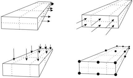
Figure 2.1: 3D discretization of a PEEC structure

2.3.2

Interpretation as equivalent circuit

To solve the integrals in (2.14), an approach that uses a concept of rectangular pulse functions is used. The structure is discretized into volume cells carrying a, throughout the volume, constant current density. The charges are supposed to be on the surfaces of the cells, and are also considered constant. The pulse functions are utilized in the PEEC models to mathematically describe this concept.

Figure 2.1 shows a 3D discretization of a rectangular conductor. The arrows indicate current direction, dashed lines separate volume cells while dotted lines separate surface cells. 1D and 2D discretization are also possible, the distinction will be the number of surface cells and the number of directions in which the currents exist. The use of 3D models should be avoided wherever possible, since the complexity significantly increases [8]. Figure 2.2 and 2.3 show a volume and a surface cell, both in one dimension, in-terpreted as equivalent circuits. The voltage sources can account for electromagnetic couplings from other cells.

2.3.3

Frequency domain circuit equations

The final frequency-domain PEEC model, which includes external sources and dielectric material, is shown in Figure 2.4. Applying Kirchhoff’s voltage and current laws to the branches and nodes of the equivalent circuit, results in the following equation system,

  −CM −(R+jωL) jωF+ST_Y L −STCTM     V IL  ₌   VS ST_I S  _, _(2.15)

which is to be solved for the unknown potentials and currents, V and IL, respectively.

(17)

facilitation, Y is an admittance matrix describing the lumped components, while VS and IS are external sources [7].

The arrangement in (2.15) is called the modified nodal analysis (MNA) method and makes it possible to extract all currents and potentials of the PEEC structure. The nodal analysis (NA) method uses another approach to solve the equivalent circuits of Figure 2.4. The NA only solves for the node potentials and is hence faster [7].

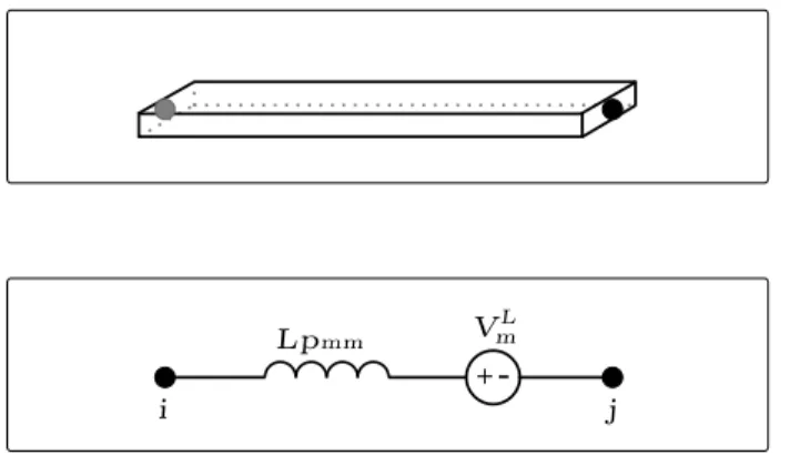
In the implementation, the MNA method is used to extract the currents from all volume cells when calculating the electromagnetic field. The NA method is used when the input terminal of the antenna is probed. This is of course also possible using MNA, but not vice versa. Volume cell Equivalent circuit (Lp)PEEC Lpmm Vm L i j

Figure 2.2: (L_p)PEEC model for a volume cell.

Surface cell Equivalent circuit (P)PEEC Vi C Pii 1 i

(18)

2.4. EISLAB’s PEEC solvers 9 Lpmm Rm i j V a C Pii 1 Pjj 1 Yij ILm

S

Paa Pia a=1 a=i N V i C VCj V a C

S

Paa Pja a=1 a=j N

S

Lpmb b=1 b=m M jw _I_Lb I_Cj I_Ci ILn IYij

Figure 2.4: (Lp,R,P)PEEC model.

2.4

EISLAB’s PEEC solvers

In the spring of 2005 Frederik Schmid finished his Master’s thesis in computer science at EISLAB [8]. The result was a PEEC solver running in Linux. It was developed in C++ using the Portable, Extensible Toolkit for Scientific Computation (PETSc) [9], an open suite of data structures and routines for applications modelled by partial differential equations. The task was to optimize experimental code developed by researchers at EIS-LAB and the EMC Laboratory of the Dept. of Electrical Engineering at the University of L’Aquila. The previous work was code fragments solving various PEEC problems, lacking consistency and means of a generic input. There was also a desire to surrender a Windows implementation that used a commercial linear-algebra package.

During the fall of 2005 Peter Anttu has done a revised implementation of the PEEC solver. PETSc has been replaced by Gmm++ [10], which is a C++ template library for matrix models and operations. Gmm turned out to be more suitable for PEEC calculations, hence a more efficient solver is now available with a clear and intuitive source code. As of today, the work is focused on making a parallel implementation that is intended to run on a computer cluster at Ume˚a University.

Both PETSc-PEEC and Gmm-PEEC have been utilized during the work of this thesis. Without going into detail, the implementations consider text files as input, describing the physical properties of the model, the existence of external components and a number of parameters affecting how the model is to be treated by the solver. The output is a text file containing the desired potentials and currents formatted in Matlab syntax.

(19)

(20)

C

HAPTER

3

Particle-swarm optimization

When dealing with optimization of engineering problems, the functions considered are often very complex, multi-dimensional and might be both continuous and discrete within the solution domain. Since calculus no longer applies, analytic evaluation can no longer be used to find points of minimum or maximum. Intuitively, the need for a smart scheme that makes guesses based on the relative solution fitness, is evident.

3.1

Background

In 1995 James Kennedy and Russell Eberhart presented particle-swarm optimization (PSO), an optimizer that models the behavior and intelligence of a swarm of bees, school of fish or flock of birds, and emphasizes both social interaction and nostalgia from the individual’s perspective.

Kennedy and Eberhart formed a research duo of a social psychologist and an electrical engineer, whose work has had a great impact on the electromagnetic community. PSO is intuitive, easy to implement and has been proven to outperform other and more intricate methods like genetic algorithms.

3.2

Genetic algorithms

A basic understanding of genetic algorithms (GAs) is preferable when dealing with other optimization techniques, thus a short introduction will be given in this section. GAs were introduced in the early 70s by John Holland, and is sprung from evolutionary computing, invented in the 60s.

GAs rely on the principals of Darwin’s theory of evolution. In optimization appli-cations the concept of survival of the fittest combined with selection and adaptation, provides robust and stochastic search methods. Being effective in optimizing complex,

(21)

multidimensional functions in a near-optimal fashion, GAs have proven successful in a vast amount of engineering problems.

Since GAs model evolution they, in essence, share paradigm with genetics. The key concepts are [11];

• Genes - A parameter is generally equivalent to a gene. Some sort of coding or mapping translates a parameter value into a gene,

• Chromosomes - A string of genes is referred to as a chromosome. In a 3D example three genes would together form a trail solution. This solution is equivalent to a chromosome or a position,

• Population - A set of solutions is called a population, • Generation - Iterations in the GA,

• Parent - A pair of existing chromosomes are selected from the population for mating or recombination,

• Child - The offspring of the parents, and

• Fitness - There must be a way to tell how fit an individual is. Often, there exists a function which given a chromosome returns a fitness value.

The main idea is to represent parameters as genes in chromosomes. Valid chromosomes are grouped in a population, from which fit parents are selected to produce new chromo-somes by recombination and mutation.

One reason for the fact that GAs are being considered complex and untidy to imple-ment, is the many options associated with the selection, recombination and mutation [12]. The PSO, on the other hand, only concerns one major operation. This operation is the velocity calculation, which will be discussed in the following sections.

3.3

Theory

Since PSO models swarm behavior, this sections takes of from a somewhat informal point of view. Imagine a swarm of bees looking for the most fertile feeding location in a field. Each bee has a location in the three-dimensional space, xm, where the parameters x1,

x2 and x3 are intended to constitute a point in space. The bee evaluates every position

for the absolute fitness. This fitness will, for this example, be a positive number which increases with increasing fertility. The bee remembers the spot where it encountered the best fitness and also shares this information with the other bees, so that the entire swarm will know the global best position. The bee’s movement is controlled by its velocity,vm, which is influenced by its best personally encountered location and the global best. The bee will always try to find the way back to its personal best location, while at the same

(22)

3.3. Theory 13

time curiously moving towards the global best. If a bee finds a location that has a fitness greater than any encountered before, the entire swarm will be informed instantly and thus move towards this location. The result will be a swarming behavior, evidently based on both nostalgia and social influence.

It should be emphasized that the algorithm is considered to be continuous, i.e. the particles’ parameters can take on any value in the defined interval. In the previous example this means that the bee can be in any position in the field, even in the exact same spot where other bees are. Another way of describing this is to state that collisions do not occur, which of course lacks correspondence in real life.

A function that evaluates the position in solution space is needed. Though the algo-rithm is generic, the fitness function is often unique to a specific problem.

More formally, the algorithm is [12]; • Define the solution space,

• Define a fitness function,

• Randomly initialize xm and vm (for particle 1 to M), • Reckon pbp

m and pbvm (for particle 1 to M), • Reckon gbp _and _gbv_{, and}

• Until some criteria are met do (for particle 1 to M): – Evaluate current position’s fitness

∗ If it is better than pbv

m, exchange pbpm and pbvm ∗ If it is better than gbv_{, exchange}_gbp _and _gbv – Reckon vm

– Letxm =xm+vm (Determine next position),

wherepbp

m is a vector pointing to the personal best position, andpbvm is the value associated with that position. gbp _and _gbv _{are in the same manner associated with the global best} position. Note that the personal position and value are related to one of theM particles, and that the global best position and value are shared, thus equal to all individuals. The dimension is of course not limited to three, but instead N.

Of consistency, the reckoning of next position should read

x(t+ ∆t)m =x(t)m+v(t)m∆t, (3.1)

though t is often omitted and ∆t is implied to be 1.

PSO is considered to be unique in the sense that it explores the space wherein the solutions exist, not a space of solutions, which is a fundamental property of GAs.

(23)

3.3.1

Change of change

The heart of the optimization is the computation of the velocity, which is analogous to the modification of the relative change, or simply change of change. The concept is to use vectors pointing from the current to the personal best and global best position, according to v(t)mn=v(t−∆t)mn+ φ1(pbpmn−xmn) +φ2(gbpn −xmn) ∆t , (3.2) where φ1 =c1rand() and φ2 =c2rand().

The constants c1 and c2 affect the influence of nostalgia and social interaction,

respec-tively, whereas rand() is a function returning a random number from a uniform distribu-tion in the interval [0,1). The calls to the random funcdistribu-tion are considered to be separate, thus making them independent. Again, implying t and ∆t= 1, a clearer representation of (3.2) is given by

vmn =vmn+φ1(pbpmn−xmn) +φ2(gbpn −xmn).

Throughout the report, the significance of φ1, φ2 and rand() will not change.

3.3.2

Craziness, explosion, inertia and constraints

Since φ1 and φ2 are stochastic, their presence models the slight unpredictable behavior,

or craziness, of particles in a swarm [13].

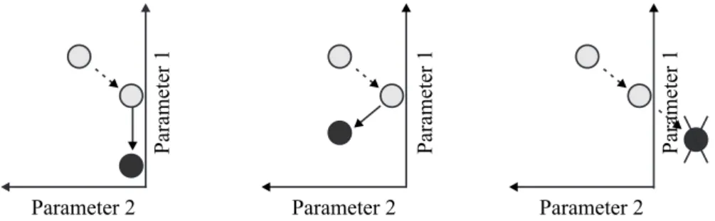
If the variables can take on any value, an oscillating behavior of increasing amplitude is likely to occur if the velocity is not constrained. This is often referred to as explosion and is avoided by limiting|vm| by the positive numbervmax.

The variables are often limited to some interval. This will introduce a need to handle particles trying to pass the boundary limits. Figure 3.1 shows three boundary conditions. The leftmost shows the absorbing-wall approach, where the velocity in the direction of the boundary is zeroed. The following condition, the bouncing-wall approach, reflects the particles while the rightmost, the invisible wall, simply lets the particles pass. An inherited condition is that no fitness evaluation will be performed beyond the boundaries. This usually reduces the number of computations drastically, since the algorithm itself is very simple compared to most fitness evaluations. Particles outside the boundaries are supposed to, on their own, find their way back to the defined space [12].

Inertial weight,w, is shown in (3.3) and was introduced for controlling the convergence of the algorithm. A largew encourages exploration, while a small w makes the particles fine-comb the area surrounding the global maximum. The inertial weight is therefor often

(24)

3.3. Theory 15

linearly decreased during an optimization, to speed up the convergence while covering a large area at the beginning.

vmn =wvmn+φ1(pbpmn−xmn) +φ2(gbpn −xmn). (3.3) The constriction factor, K, was introduced to make an analytical analysis of the PSO, though (3.4) can be considered a special case of (3.3) [12].

vmn=K(vmn+ϕ1rand()(pbpmn−xmn) +ϕ2rand()(gnbp−xmn)), (3.4) where K is determined from

ϕ=ϕ1+ϕ2;ϕ >4 (3.5)

and

K = 2

|2−ϕ−pϕ2 ₋₄_ϕ_|. (3.6)

Combinations of empirical testing and mathematical analysis of various test cases, by means of parameter settings, are summarized in [12]. The suggested settings are

c1 = 1.49, c2 = 1.49, and that wis linearly decreased from 0.9 to 0.4, or that K = 0.729,

ϕ1 = 2.8 and ϕ2 = 1.3, depending on method of implementation.

Overall, a population size of ≤30, using the invisible-wall approach with the settings displayed, has proven to provide good results [12].

Parameter 2 Parameter1 Parameter 2 Parameter1 Parameter 2 Parameter1

Figure 3.1: Boundary conditions in the PSO algorithm.

3.3.3

Matrix representation

In [14], a matrix representation of the particle swarm is proposed. The M positions, velocities and personal best locations, all in N dimensions, are gathered in the M ×N

(25)

matrices, X, V and P, as described in (3.7), (3.8) and (3.9), respectively. X =      x11 x12 . . . x1N x21 x22 . . . x2N ... xM1 xM2 . . . xM N      (3.7) V=      v11 v12 . . . v1N v21 v22 . . . v2N ... vM1 vM2 . . . vM N      (3.8) P=      p11 p12 . . . p1N p21 p22 . . . p2N ... pM1 pM2 . . . pM N      (3.9)

The global best is still represented by a vector, but is referred to as a 1×N matrix,

G=£ g1 g2 . . . gN

¤ .

The matrix representation leads to a very elegant expression for the new position of all particles,

X =X+V.

The velocity matrix must still be updated element by element as,

vmn =vmn+φ1(pmn−xmn) +φ2(gn−xmn), to retain the intended behavior.

Note that this is exactly what has been described in the previous section, though the value associated with each position is implied, and therefor the need for distinction between vector and scalar is no longer necessary.

3.4

Discrete binary representation

In [15], a clever technique for making the particle swarm and its operations binary is introduced. This implementation distinguishes the solution space from the coding space and uses a binary implementation of the position vectors, wherexm = [01. . . xmN],pm = [00. . . pmN] and gm = [10. . . gN] .

The velocity is given by

vmn =vmn+φ1(pmn−xmn) +φ2(gn−xmn), (3.10) where the velocity isnot a binary number.

(26)

3.4. Discrete binary representation 17

3.4.1

Change of change of change

While the update of the velocity according to (3.10) stays the same, compared to that of the continuous version, the interpretation is now that velocity is the probability of a bit taking on a one or a zero. The meaning of the change of change is therefor evidently different. This is implemented as an IF statement,

IF (rand() < S(vmn)) THENxmn= 1 ELSExmn = 0, where

S(vmn) = 1

1 +e−vmn, (3.11)

is called a sigmoid limiting transformation [15].

This leads to the conclusion that the probability of a bit taking on a one is S(vmn), and 1−S(vmn) that it will be a zero. Since this holds regardless of the initial state of a bit, the probability of a bit changing must be S(vmn)(1−S(vmn)). Note that this only holds if the initial state of a bit is unknown. This is represented in [15] as

p(∆) =S(vmn)(1−S(vmn)). (3.12) Thus a change in the velocity still is a change in the rate of change [15].

3.4.2

Gray coding

Initial testing of function optimization showed that the particles often converged on a spot near the global best, and that they never tended to find the global best, no matter how many iterations that were performed. The cause is easily realized if the distance in coding space is considered.

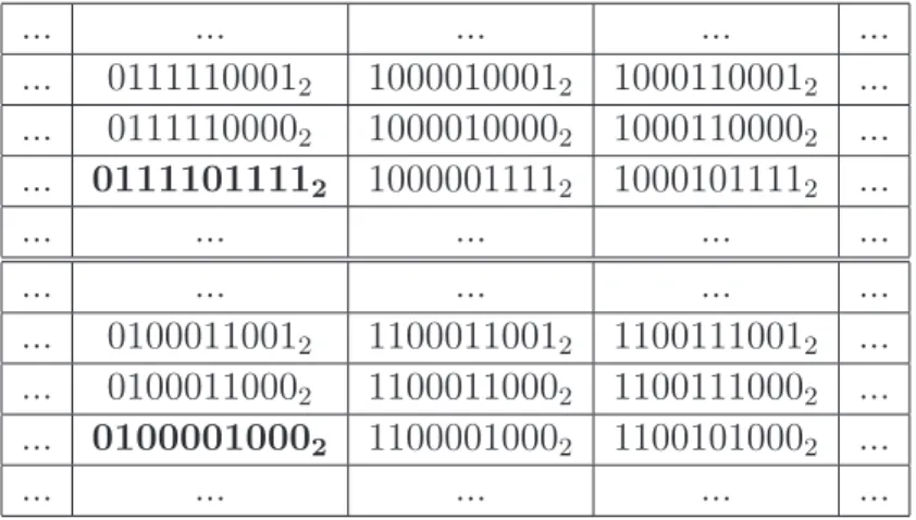
In Table 1, the fitness of a solution space is illustrated. Table 2 shows two different representations of the coding space, related to the solution space in Table 1.

If the algorithm used the the first representation in Table 2 and ended up on the position marked with bold figures, it would take a probability of all bits changing to end up on the global best, which of course is very low. In fact, it is a chance so slim that it can never be expected that the algorithm finds the global maximum. If, on the other hand, the second representation is used, only two bits need to change for the algorithm to find the global maximum.

To circumvent this problem, the desired mapping from coding to solution space is one that considers a short Hamming distance to represent a short distance in the solution space. On way of achieving this is to use a reflected binary Gray code shown in Table 3. The first implementation discussed uses a binary representation of increasing decimal numbers, while the second uses Gray code. The advantage is that adjacent positions will differ with a maximum Hamming distance of 2. One bit change does however not mean that an equivalent move of length one is executed, but it definitely makes the algorithm explore the space more freely.

(27)

Table 1: Fitness of the solution space. ... ... ... ... ... ... 0.88 0.94 0.88 ... ... 0.94 1.00 0.94 ... ... 0.88 0.94 0.88 ... ... ... ... ... ...

Table 2: Initial and Gray-code representation of coding space.

... ... ... ... ... ... 01111100012 10000100012 10001100012 ... ... 01111100002 10000100002 10001100002 ... ... 01111011112 10000011112 10001011112 ... ... ... ... ... ... ... ... ... ... ... ... 01000110012 11000110012 11001110012 ... ... 01000110002 11000110002 11001110002 ... ... 01000010002 11000010002 11001010002 ... ... ... ... ... ...

Table 3: Gray codes with corresponding decimal numbers.

Dec. Bin. Dec. Bin. Dec. Bin. Dec. Bin. 0 000002 8 011002 16 110002 24 101002 1 000012 9 011012 17 110012 25 101012 2 000112 10 011112 18 110112 26 101112 3 000102 11 011102 19 110102 27 101102 4 001102 12 010102 20 111102 28 100102 5 001112 13 010112 21 111112 29 100112 6 001012 14 010012 22 111012 30 100012 7 001002 15 010002 23 111002 31 100002

(28)

C

HAPTER

4

Electromagnetic field and

antenna parameters

When dealing with antennas, the radiated electromagnetic field is of great importance. Analytic evaluations are, however, often very cumbersome, even if extensive simplifi-cations are made. In this chapter, a numerical method for calculating the radiated electromagnetic field from a PEEC structure is discussed.

4.1

The spherical coordinate system

In the orthogonal implementation of PEEC, all volume elements will be in the direction of either one of the base vectors in the cartesian coordinate system. If the volume cells are treated as short dipoles, generally known as Hertzian dipoles, convenient ways of calculating the electric field exist.

In Figure 4.1 a point in space, P, is represented. The vector pointing to P can be represented by r = rxi+ryj +rzk or r = rReR +rθeθ +rφeφ. From the figure it is determined that rx = rRsinθcosφ = Rsinθcosφ, ry = rRsinθsinφ = Rsinθsinφ and

rz = rRcosθ = Rcosθ. From this, expressions converting from spherical to cartesian coordinates can be gathered in a matrix, allowing for conversions according to

  a_ax_y az  ₌ 

 sin_sinθ_θcos_sin_φφ cos_cosθ_θcos_sin_φφ −_cossin_φφ

cosθ −sinθ 0     a_aR_θ aφ  _,

where a is converted to a cartesian representaion.

(29)

Figure 4.1: Definition of base vectors from [16].

4.2

Electromagnetic field from a Hertzian dipole

In the far field of a Hertzian dipole the electric and magnetic field are completely in phase. It can be shown that they, for an infinitesimal current element in the direction of

k, can be described by [6]

Eθ =Z0

jIzd`zβ 4πrdist

sinθe−jβrdist (4.1)

and

Hφ =

jIzd`zβ 4πrdist

sinθe−jβrdist, (4.2)

whereZ0 = 120 Ω is the free-space impedance,Iz the current, d`the infinitesimal length, and β = ω/c = 2πf /c is the wave number. The distance between the observer and the center of the dipole is represented by rdist.

If the current is considered constant, the expressions for an infinitely thin dipole of finite lengthlz, placed at the origin and in the direction of k, will be

Eθ =Z0

jIz`zβ 4πrdist

sinθe−jβrdist _(4.3)

and

Hφ=

jIz`zβ 4πrdist

sinθe−jβrdist_. _(4.4)

In similar fashion, the electric field radiating from a short dipole, placed in the direction of i, will be

Eφ=−Z0

jIx`xβ 4πrdist

(30)

4.3. Antenna parameters 21

and if placed in the direction of j,

Eφ=−Z0

jIy`yβ 4πrdist

cosφe−jβrdist_. _(4.6)

Letting the PEEC solver use the MNA method yields the current and potential of each volume and surface cell, respectively. By utilizing the currents and knowing the position,

r0

k, and size of each volume cell, superpositioning of the electric field in a point, r, from K volume cells is given by

E(r) =       ER(r) Eθ(r) Eφ(r)      = K X k=1         0 Z0jI z k`zkβ 4πrdist k sinθe −jβrdist k −Z0jI x k`xkβ 4πrdist k sinφe −jβrdist k −Z₀jI y k` y kβ 4πrdist k cosφe −jβrkdist         (4.7) whererdist

k =|r0k−r|. Ikx,Iky andIkz are currents in the direction ofi,jandk, respectively. Each volume cell holds a current vector

Ik =       Ix k I_ky Iz k       (4.8)

in which only one element is non-zero. This makes it possible to use (4.7) to sum over all K elements. The resultant field is meant to be converted to a representation in the cartesian coordinate system.

While the expression for Eθ holds for any point of observation, the expressions for

Eφ are considered special cases for when the point of observation is on the plane of ij. Consistent evaluation of antennas is therefor limited to structures discretezied in the axis of k.

4.2.1

Extraction of currents

The Gmm-PEEC solver has been configured to return the information needed to calculate the electromagnetic field. The solver was modified to always include the min and max coordinate, and the direction of the current for each volume cell. In MNA mode, the vector containing VandILof (2.15) is returned, thus making the current for each source element available.

4.3

Antenna parameters

The radiated power and its pattern are important indications of an antenna’s properties. Some measures of antenna performance are defined in this section, which originate from

(31)

[6].

The power of an electromagnetic field is given by the time-average of the Poynting vector

Pavg =<(E×H∗), (4.9)

where the E and H fields are considered to be represented by their effective or RMS value.

The radiation intensity U(θ, φ) is defined as time-averaged power per unit solid angle as U(θ, φ)≡ dPrad dΩ =r 2_|_P avg|=r2|<(E×H∗)|= r 2 Z0 ||E|2|. (4.10) The directive gain Dgain(θ, φ) of an antenna is defined as the ratio of the radiation intensity to that of an isotropic radiator. An isotropic radiator is a hypothetical antenna that radiates the same total power at any point on a hypothetical sphere surrounding it as U0 = Prad 4π , (4.11) yielding Dgain(θ, φ) = U(θ, φ) U0 = 4πU(θ, φ) Prad . (4.12)

If the radiated power is considered to be equal to the power received by the antenna, the directive gain is given by

Dgain(θ, φ) = 4πU(θ, φ) Pin = 4πU(θ, φ) <(VinI∗in) , (4.13)

where Vin and Iin are complex phasors of the voltage and current at the feeding point. The asterisk, ∗_{, indicates that the current is represented by its complex conjugate.}

Di-rectivity of an antenna is considered to be the maximum value of its directive gain. The gain is often expressed in decibels, where

GdB(θ, φ) = 10 log10Dgain(θ, φ), (4.14) still under the assumption that Prad =Pin.

Another factor considered is the return loss, S11. It is defined as the ratio of the

re-flected wave to that of the outgoing, experienced by the generator supplying the antenna. The return loss can be evaluated considering the impedances of the transmission line, connecting the generator and the antenna, and the impedance of the feeding point, where

S11=

Zantenna−Zcoax

Zantenna+Zcoax

. (4.15)

Common impedances of coaxial cables, used as transmission lines, are 50 and 75 Ω. It is desired to keep S11 as close to 0 as possible, thus matching the antenna with the feed

(32)

4.4. Verification of method 23

4.4

Verification of method

The PEEC solver was configured to model a long dipole, consisting of two rectangular bars. The bars are each 10 cm long, with a cross-sectional area of 10−10 _cm2_{. A 1A}

sinusoidal source at the origin connects the bars which expand on the axis ofi, in opposite direction.

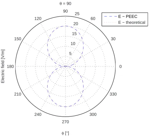
Each bar is discretisized 50 times into 50 volume cells, in the direction of i, and the antenna is fed at its theoretical resonant frequency of 750 MHz. The absolute value of the electric field at a distance of 3 m from the origin is observed. Figure 4.2 shows the absolute value of the electric field from the PEEC structure compared to that of a theoretical long dipole. The expressions for the theoretical long dipole originate from [17], where the theoretical intensity is determined to 20 V/m, for this particular example. The result from the superpositioning of the electric field, radiating from the 100 short dipoles in the PEEC structure, was a maximum field intensity of 20.082 V/m, which implies a deviation of 0.4 %. 5 10 15 20 25 30 210 60 240 90 270 120 300 150 330 180 0 θ = 90 φ [°] Electric field [V/m] E − PEEC E − theoretical

(33)

(34)

C

HAPTER

5

Implementation

This chapter presents an implementation of the PSO algorithm optimizing both known and unknown functions. The PSO algorithm has been implemented in Matlab. The electromagnetic structures are modelled using PETSc-PEEC and Gmm-PEEC, and the result is postprocessed in Matlab. The algorithm is implemented in its binary guise and the antennas being evaluated are a binary patch and a dipole array.

5.1

Building blocks

The heart of the implementation is PSO.m which incorporates a binary version of the PSO. When a particle is to be evaluated for fitness a binary vector is passed to Binary-Patch.m.

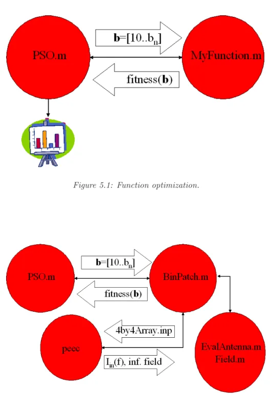
BinaryPatch.m takes two additional arguments, telling whether the optimization should be visualized and if the PEEC solver should use the MNA or the NA method. Binary-Patch.m creates an input file to the PEEC solver, runs the external solver and evaluates the fitness, which is returned to the calling function. If the optimization is to be visual, the binary vector is passed to MyFunction.m which returns a fitness for a mathematical function as shown in Figure 5.1.

In the case of electromagnetic optimization, shown in Figure 5.2, BinaryPatch.m eval-uates the impedance of the structure or the electromagnetic field. The latter is done by a call to EvalAntenna.m which returns the maximum directive gain, found in two horizontal planes, and the return loss. EvalAntenna.m calls Field.m, which implements the methods described in Chapter 4.

The electromagnetic problems are represented by binary patches, of which the PSO algorithm can alter the physical representations. Figure 5.3 shows the patch represented by b= [1000011000110011]. The lower left corner is represented by the first entry of b. The next position to the right, is the next entry. The positions are incremented row-wise,

(35)

up to the top right corner, represented by the last entry of b.

Appendix A contains the Matlab code of the functions mentioned in this section.

Figure 5.1: Function optimization.

(36)

5.2. Optimization of a known function 27

m

Figure 5.3: Example of a 4-by-4 patch antenna. The feeding point is indicated by the ring.

5.2

Optimization of a known function

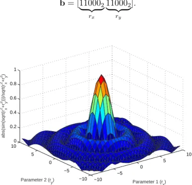
To visualize the activities of the algorithm the optimizer was set to find the maximum of a polar sinc function,

rz = |sinpr2 x+ry2| p r2 x+r2y , (5.1)

shown in figure 5.4. The length of the binary vector is set to ten and two five-bit numbers are used to represent a position, where

b= [11000_{| {z }}2 rx 110002 | {z } ry ]. −10 −5 0 5 10 −10 −5 0 5 10 0 0.2 0.4 0.6 0.8 1 Parameter 1 (r_x) Parameter 2 (r_y) abs(sin(sqrt(r x 2+r y 2)))/sqrt(r x 2+r y 2)

(37)

The numbers in b are interpreted as Gray code, as discussed in Chapter 3. Figure 5.5, 5.6 and 5.7 show the progress of the optimization, and that the algorithm eventually finds the global maximum of the function. If two or more particles end up in the same spot, their individual fitness values are added, indicating that there exist nine particles at the global maximum in figure 5.7. Note that the figure is scaled to show the particles’ added fitness. −10 −5 0 5 −10 −5 0 5 0 0.2 0.4 0.6 0.8 1 Parameter 1 (r_x) Parameter 2 (r_y) abs(sin(sqrt(r x 2+r y 2)))/sqrt(r x 2+r y 2)

(38)

5.2. Optimization of a known function 29 −10 −5 0 5 −10 −5 0 5 0 0.2 0.4 0.6 0.8 1 Parameter 1 (r_x) Parameter 2 (r_y) abs(sin(sqrt(r x 2+r y 2)))/sqrt(r x 2+r y 2)

Figure 5.6: Particle locations after ten iterations.

−10 −5 0 5 −10 −5 0 5 0 2 4 6 8 10 Parameter 1 (r_x) X= 0 Y= 0 Z= 9 Parameter 2 (r_y) abs(sin(sqrt(r x 2+r y 2)))/sqrt(r x 2+r y 2)

(39)

(40)

C

HAPTER

6

Results

6.1

Antenna optimization

Antennas are very untidy to handle by means of mathematical analysis. Instead, the an-tennas will be treated as composed of many infinitesimal dipoles, as previously discussed. This section considers a patch antenna that is placed at the origin in the ij-plane. The PSO controls the input to the PEEC solver and can hence alter the physical description of the antenna structures. The patch antenna is fed by a 1A current source in parallel with a 50 Ω resistor, representing a coaxial cable. The target for the PSO is to optimize resonant frequency.

The other configuration considered is an array of two long dipoles, with variable dis-tance between the dipoles. Here, the electric-field strength is evaluated, and the directive gain is optimized.

6.1.1

Optimization of resonant frequency

As a first example, a resonant-frequency optimization of a binary patch antenna is per-formed. The target is a full binary patch of size 4 by 4 cm fed at (1,1), as shown in figure 6.1, together with the 1 A current source and the 50 Ω resistor. The absolute value of the current (bottom) flowing into the antenna, and the potential (top) of the feeding point are shown in Figure 6.2. The current and potential are assumed to have zero phase, i.e. be real-valued, at the resonant frequencies.

The fitness function was set to count the number of resonant frequencies, by examining the derivative of |Iin|. A structure not having exactly two resonant frequencies, as the target, was given a fitness of 0. All other structures are given a fitness equal to 1 minus the deviation of each resonant frequency from the target’s of 1.9 and 4 GHz. Any negative

(41)

fitness is set to 0. The target is considered an invalid configuration, as is any configuration not having a PEEC cell adjacent to the feeding point.

1A _{50 ohm}

Patch antenna

Figure 6.1: Model setup of the patch antenna.

0 0.5 1 1.5 2 2.5 3 3.5 4 4.5 5 0 10 20 30 40 50 Freq. [GHz] Abs(V in ) [V] 0 0.5 1 1.5 2 2.5 3 3.5 4 4.5 5 0 0.2 0.4 0.6 0.8 1 Freq. [GHz] Abs(I in ) [A]

Figure 6.2: Input current (bottom) and input voltage (top) at the feed of the reference antenna.

(42)

6.1. Antenna optimization 33

1 and 2 show extracts from the log file. The rows in X hold current position of the particles while the rows inPshow the personal best, according to Section 3.3.3. The left and right fitness column show current and personal best fitness, respectively. Line one of each extract shows which particle whose personal best is constituting the global best. The antenna b = [0101111000101010], was obviously found to be most fit and its characteristics are shown in Figure 6.3. It is evident that the optimized antenna has the desired resonant frequencies at 1.9 and 4 GHz. Since this antenna is physically smaller than the reference, this optimization could also be considered aiming at low weight.

Table 1: The first iteration of the resonant-frequency optimization.

Iteration: 1 Global best: Particle 8

X(1,:): 1000000001101000 Fitness:0.636 P(1,:): 1000000001101000 Fitness:0.636 X(2,:): 1011110010000011 Fitness:0.000 P(2,:): 1011110010000011 Fitness:0.000 X(3,:): 0000110001111110 Fitness:0.768 P(3,:): 0000110001111110 Fitness:0.768 X(4,:): 0111101001110100 Fitness:0.000 P(4,:): 0111101001110100 Fitness:0.000 X(5,:): 0000011001111100 Fitness:0.000 P(5,:): 0000011001111100 Fitness:0.000 X(6,:): 0110110101010110 Fitness:0.000 P(6,:): 0110110101010110 Fitness:0.000 X(7,:): 0100000010001101 Fitness:0.000 P(7,:): 0100000010001101 Fitness:0.000 X(8,:): 0111101110101110 Fitness:0.972 P(8,:): 0111101110101110 Fitness:0.972 X(9,:): 0100100000001011 Fitness:0.000 P(9,:): 0100100000001011 Fitness:0.000 X(10,:):0010011010111000 Fitness:0.000 P(10,:):0010011010111000 Fitness:0.000

Table 2: The last iteration of the resonant-frequency optimization.

(43)

0 0.5 1 1.5 2 2.5 3 3.5 4 4.5 5 0 10 20 30 40 50 Freq. [GHz] Abs(V in ) [V] 0 0.5 1 1.5 2 2.5 3 3.5 4 4.5 5 0 0.2 0.4 0.6 0.8 1 Freq. [GHz] Abs(I in ) [A]

Figure 6.3: Input current (bottom) and input voltage (top) at the feed of the optimized patch antenna.

6.1.2

Optimization of the electric-field strength

The patch antennas turned out to be complicated to model, when it comes to field optimization. However, since the dipole was proven to be modelled with good results, an array with such elements replaces the patch antenna for this purpose. BinPatch.m has been replaced by BinDipole.m, but works conceptually in the same way. Figure 6.4 shows the array used for the electric-field optimization, wherea represents the length of the dipoles and b half the distance between them. The total distance, or 2b, is labelled

d.

The PEEC solver is used to model two dipoles of the same kind that was mentioned in Chapter 4, i.e. a = 20 cm or, equivalently, λ/2 for the intended frequency of 750 MHz. The distinction from the previous dipole model, is that the dipoles are placed in the direction of k, instead of i, and that the elements are interconnected by two electromagnetically shielded 0 Ω cables, modelled by two 10−3 _{Ω resistors.}

The directivity is evaluated in the planes of jk and ij. The variable b is controlled by the PSO, using a five-bit binary number, interpreted as Gray code. The distance is varied between 0 and λin 32 steps, while the directivity is being optimized. Table 3 and 4 show extracts from the log file. When the run was terminated after 10 iterations, the best fitness had been discovered by particle one to nine. 011112 interpreted as Gray code

(44)

6.1. Antenna optimization 35

b

a

k

j

0

a

d

1A

Figure 6.4: Model setup of the dipole array.

Table 3: The first iteration of the directivity optimization.

represents 10, which implies that the distance is b = 10λ/31⇒d = 20λ/31. This result agrees well with the theoretical two-dipole array [18], where the maximum directive gain is found when d= 2λ/3. Ifd is manually configured to 2λ/3, the directivity found from the array modelled by the PEEC solver is 4.68 or 6.87 dB. Figure 6.5 shows the electric field intensity at a distance of three meters from the array. The figure is showing the plane of ij, in which the maximum directive gain was found.

(45)

Table 4: The last iteration of the directivity optimization.

X(1,:): 00111 Fitness:3.914 P(1,:): 01111 Fitness:6.868 X(2,:): 01111 Fitness:6.868 P(2,:): 01111 Fitness:6.868 X(3,:): 01111 Fitness:6.868 P(3,:): 01111 Fitness:6.868 X(4,:): 01111 Fitness:6.868 P(4,:): 01111 Fitness:6.868 X(5,:): 01111 Fitness:6.868 P(5,:): 01111 Fitness:6.868 X(6,:): 01111 Fitness:6.868 P(6,:): 01111 Fitness:6.868 X(7,:): 01111 Fitness:6.868 P(7,:): 01111 Fitness:6.868 X(8,:): 01111 Fitness:6.868 P(8,:): 01111 Fitness:6.868 X(9,:): 01111 Fitness:6.868 P(9,:): 01111 Fitness:6.868 X(10,:):01011 Fitness:6.311 P(10,:):01011 Fitness:6.311 5 10 15 20 25 30 210 60 240 90 270 120 300 150 330 180 0 θ = 90 φ [°] Electric field [V/m]

E − Dipole array from PEEC model

(46)

C

HAPTER

7

Conclusions and further work

7.1

Conclusions

The thesis presents how to combine the PSO algorithm with a PEEC-based electromag-netic solver, for the purpose of optimizing antenna structures. The intuitive behavior of the PSO algorithm was easily implemented and the result was overall very good. The merging of the existing PEEC solvers and the particle-swarm optimization algorithm turned out to be successful. The results indicate that the optimization is not limited to antennas, but could also be used for inverse problems and the design of micro-strip filters.

The field calculation turned out to be very tedious, since the extraction of currents never were intended while the structure of the object-oriented code was developed. Due to the definition of the spherical coordinate system, the results are only valid if the structures are 1-dimensional in the plane of ik orjk, or if the point of observation lies in the plane of ij for 3D structures. This is something that should be taken care of before using the resulting code as a generic optimizer.

The behavior was stable and the activities of the algorithm can be viewed and back-tracked, by the use of a log.

It should be noted that the attached Matlab code is to be considered a draft, though it hopefully will be an aid for others interested in implementing the algorithm.

7.2

Further work

The first improvement would be to endow the PSO algorithm with a memory for the fitness of a certain antenna configuration. Since the structures being used in this thesis are relatively small, the penalty for evaluating the same configuration multiple times does

(47)

not degrade the overall performance significantly. For larger structures, it would however not be acceptable to reevaluate multi-hour runs.

It would be interesting to include an implementation of the genetic algorithm and thus be able to compare their progress. An elaborate investigation of how the PSO parameters affect this particular antenna optimization is also of interest.

The field evaluation of the dipole array was used mainly to show that the field op-timization works. The initial idea of optimizing patch antennas did not turn out as expected, as was therefor partly abandoned. Since the patch antennas are important in the current research projects at EISLAB, the work involving modelling of these antennas will continue.

I have been advised to change the core of the binary version of the PSO. This proposal would make the movement equivalent to that of the continuous version and would preserve the swarming behavior of the particles. The concept is to use an alternate version of the presented Gray code and has, to my knowledge, never been implemented.

(48)

A

PPENDIX

A

Matlab code

PSO.m: 0001 clear all; 0002if(length(strfind(path,’/mypeec/common’))==0) 0003 path(path,’~/mypeec/common/’); 0004end

0005 RAND(’state’,sum(100*clock))%Do not use pseudo-random numbers 0006 numOfParticles=10;

0007 numOfIterations=40;

0008 sizeOfArray=16;%Initialize the size 0009 fid0=fopen(’log.txt’,’w’); 0010 visual=0;

0011ifvisual==1

0012 [x,y]=meshgrid([-10:0.625:9.75],[-10:0.625:9.75]); 0013 r=sqrt(x.^2+y.^2)+eps;

0014 z=abs(sin(r))./r;%Radial sinc function 0015end 0016 Vmax=6; 0017 w=0.729; 0018 c1=1.494;c2=1.494; 0019 mode=’MNA’; 0020 X=zeros(numOfParticles,sizeOfArray+1); 0021 X(:,1:sizeOfArray)=round(rand(numOfParticles,sizeOfArray)); 0022forparticle=1:numOfParticles%Check for invalid configurations 0023 ifX(particle,1)==0&&X(particle,2)==0&&... 0024 X(particle,5)==0&&X(particle,6)==0 0025 X(particle,1)=1; 0026 elseifX(particle,1:sizeOfArray)==ones(1,sizeOfArray) 0027 X(particle,1)=0; 0028 end 0029end 0030 Xnext=zeros(size(X)); 0031 tempBest=0;%zeros(numOfParticles,1); 0032 V=rand(numOfParticles,sizeOfArray)*Vmax*2-Vmax; 0033 P=zeros(numOfParticles,sizeOfArray+1);

0034 P(:,1:sizeOfArray)=X(:,1:sizeOfArray);%Let all particles have 0035%a location for their personal best

0036forparticle=1:numOfParticles%Let all particles have 0037 %a fitness value for their personal best 0038 ifvisual==1

0039 P(particle,sizeOfArray+1)=...

0040 BinPatch(P(particle,1:sizeOfArray),’visual’); 0041 else

0042 P(particle,sizeOfArray+1)=...

0043 BinPatch(P(particle,1:sizeOfArray),’antenna’,mode); 0044 end

0045end

0046 gBest=find(P(:,sizeOfArray+1)==max(P(:,sizeOfArray+1)));%gBest 0047%represents a row in the P matrix

0048 gBest=gBest(1);%If two or more particles represent equally 0049 %fit locations, use the first one

0050 X(:,sizeOfArray+1)=P(:,sizeOfArray+1);%Since the current fitness is 0051 %printed to the log, a value is 0052 %needed.

0053%End of initialization 0054foriteration=1:numOfIterations

0055 fprintf(fid0,’Iteration: %i Global best: Particle %i\n’,...

(49)

0056 iteration,gBest);%Print to the log 0057 forparticle=1:numOfParticles

0058 ifparticle<10

0059 fprintf(fid0,’X(%i,:): ’,particle); 0060 else

0061 fprintf(fid0,’X(%i,:):’,particle); 0062 end 0063 forn=1:sizeOfArray 0064 ifX(particle,n)==1 0065 fprintf(fid0,’1’); 0066 else 0067 fprintf(fid0,’0’); 0068 end 0069 end 0070 ifparticle<10

0071 fprintf(fid0,’ Fitness:%.3f P(%i,:): ’,...

0072 X(particle,sizeOfArray+1),particle); 0073 else

0074 fprintf(fid0,’ Fitness:%.3f P(%i,:):’,...

0075 X(particle,sizeOfArray+1),particle); 0076 end 0077 forn=1:sizeOfArray 0078 ifP(particle,n)==1 0079 fprintf(fid0,’1’); 0080 else 0081 fprintf(fid0,’0’); 0082 end 0083 end

0084 fprintf(fid0,’ Fitness:%.3f’,P(particle,sizeOfArray+1)); 0085 fprintf(fid0,’\n’);

0086 end

0087 forparticle=1:numOfParticles%Recon vmn 0088 VTemp=w*V(particle,:)+rand()*c1*... 0089 (P(particle,1:sizeOfArray)-X(particle,1:sizeOfArray))+rand()*c2*... 0090 (P(gBest,1:sizeOfArray)-X(particle,1:sizeOfArray)); 0091 ifVTemp>Vmax 0092 V(particle,:)=Vmax; 0093 elseifVTemp<-Vmax 0094 V(particle,:)=-Vmax; 0095 else 0096 V(particle,:)=VTemp; 0097 end 0098 end 0099 forparticle=1:numOfParticles 0100 forn=1:sizeOfArray

0101 ifrand()<1/(1+exp(-V(particle,n)))%Logistic function 0102 Xnext(particle,n)=1; 0103 else 0104 Xnext(particle,n)=0; 0105 end 0106 end 0107 end

0108 forparticle=1:numOfParticles%Check for invalid configurations 0109 ifXnext(particle,1)==0&&Xnext(particle,2)==0&&... 0110 Xnext(particle,5)==0&&Xnext(particle,6)==0 0111 Xnext(particle,1)=1; 0112 elseifXnext(particle,1:sizeOfArray)==ones(1,sizeOfArray) 0113 Xnext(particle,1)=0; 0114 end 0115 end 0116 forparticle=1:numOfParticles 0117 ifvisual==1

0118 tempBest = BinPatch(Xnext(particle,1:sizeOfArray),’visual’); 0119 else

0120 tempBest = BinPatch(Xnext(particle,1:sizeOfArray),’antenna’,mode); 0121 end 0122 iftempBest > P(particle,sizeOfArray+1) 0123 P(particle,sizeOfArray+1)=tempBest; 0124 P(particle,1:sizeOfArray)=Xnext(particle,1:sizeOfArray); 0125 end 0126 iftempBest > P(gBest,sizeOfArray+1) 0127 gBest = particle; 0128 end

0129 Xnext(particle,sizeOfArray+1)=tempBest;%Save current fitness in the log 0130 end

0131 X=Xnext; 0132

0133 %Start of visualization section 0134 0135 ifvisual==1 0136 particleLoc=NaN(size(y)); 0137 forparticle=1:numOfParticles 0138 xbin=[];ybin=[]; 0139 forcount=1:sizeOfArray/2 0140 ifX(particle,count)==1

(50)

41 0141 xbin=[xbin’1’]; 0142 else 0143 xbin=[xbin’0’]; 0144 end 0145 end 0146 xpos=gray2dec(xbin); 0147 forcount=sizeOfArray/2+1:sizeOfArray 0148 ifX(particle,count)==1 0149 ybin=[ybin’1’]; 0150 else 0151 ybin=[ybin’0’]; 0152 end 0153 end 0154 ypos=gray2dec(ybin); 0155 if(isnan(particleLoc(ypos+1,xpos+1))) 0156 particleLoc(ypos+1,xpos+1)=z(ypos+1,xpos+1); 0157 else 0158 particleLoc(ypos+1,xpos+1)=... 0159 particleLoc(ypos+1,xpos+1)+z(ypos+1,xpos+1); 0160 end 0161 end 0162 contour3(x,y,z);hold on;

0163 xlabel(’Parameter 1 (r x)’);ylabel(’Parameter 2 (r y)’); 0164 zlabel(’abs(sin(sqrt(r x^2+r y^2)))/sqrt(r x^2+r y^2)’); 0165 stem3(x,y,particleLoc);hold off;

0166 pause(0.1); 0167 end

0168end

0169 fclose(fid0);%Close log

BinPatch.m:

0001functionfitness = BinPatch(varargin) 0002 b=varargin{1}; 0003 MNA=0; 0004iflength(varargin)>1&&strcmp(upper(varargin(1,2)),’VISUAL’) 0005 fitness=MyFunction(b); 0006 return 0007end 0008iflength(varargin)>2&&strcmp(upper(varargin(1,3)),’MNA’) 0009 MNA=1; 0010end 0011 0012ifb(1)==0&&b(2)==0&&b(5)==0&&b(6)==0 0013 error(’Invalid location of current source’) 0014end

0015ifb==ones(1,16)%This is the reference 0016 error(’Reference antenna found’) 0017end

0018 fid0=fopen(’Geometry.inp’,’w’); 0019 squareSize=1;thickness=1e-2;%[cm] 0020 sigma=574e6;

0021 fprintf(fid0,[’number of bars ’num2str(sum(b))’\n’]); 0022forcount = 1:sum(b)

0023 fprintf(fid0,’ndiva 2 ndivb 2 ndivc 0 thinthickness yes\n’); 0024end

0025%.cs sigma 574e6

0026%.bz 0 0 0 1 0 0 0 1 0 1 1 0 0 0 1e-9 1 0 1e-9 1 1 1e-9 0027% ^z ^y p7 p8 0028% | / /| /| 0029% |/ / | / | 0030% | >x p5 / p3 /p6 |p4 0031% | / | / 0032% | / | / 0033% |/ |/ 0034% p1 p2 0035 z=0; 0036fory = 0:sqrt(length(b))-1 0037 forx = 0:sqrt(length(b))-1 0038 if(b(x+1+y*(sqrt(length(b))))==1) 0039 p1to4=[num2str(x*squareSize) ’ ’... 0040 num2str(y*squareSize)’ ’... 0041 num2str(z*squareSize)’ ’... 0042 num2str((x+1)*squareSize)’ ’... 0043 num2str(y*squareSize)’ ’... 0044 num2str(z*squareSize)’ ’... 0045 num2str(x*squareSize)’ ’... 0046 num2str((y+1)*squareSize)’ ’... 0047 num2str(z*squareSize)’ ’... 0048 num2str((x+1)*squareSize)’ ’... 0049 num2str((y+1)*squareSize)’ ’... 0050 num2str(z*squareSize)]; 0051 p5to8=[num2str(x*squareSize) ’ ’... 0052 num2str(y*squareSize)’ ’... 0053 num2str((z+thickness)*squareSize)’ ’...

(51)

0054 num2str((x+1)*squareSize)’ ’... 0055 num2str(y*squareSize)’ ’... 0056 num2str((z+thickness)*squareSize)... 0057 ’ ’num2str(x*squareSize)’ ’... 0058 num2str((y+1)*squareSize)’ ’... 0059 num2str((z+thickness)*squareSize)... 0060 ’ ’num2str((x+1)*squareSize)... 0061 ’ ’num2str((y+1)*squareSize)’ ’... 0062 num2str((z+thickness)*squareSize)];

0063 fprintf(fid0,[’.cs sigma ’num2str(sigma,’%e’)’\n’]); 0064 fprintf(fid0,[’.bz ’p1to4’ ’p5to8’\n’]); 0065 end

0066 end

0067end

0068 fclose(fid0);

0069 unix(’rm 4by4Array.inp’);

0070if(MNA)%Get the E field for one frequency (the first in samples) 0071 clear Vin;

0072 unix(’rm dump.out’); 0073 unix(’rm dump.m’); 0074 unix(’rm peec.m’);

0075 unix(’cat Geometry.inp Part2MNA.inp > 4by4Array.inp’); 0076 unix(’~/peec/src/peec 4by4Array.inp > dump.out’); 0077 run(’peec’)%run peec.m

0078 %peec.m contains the probe data, the frequencies (samples),

0079 %the coordinates repr. min and max of the volume cells, Xmin and Xmax, and 0080 %the normalized direction of each current, I.

0081 fid0=fopen(’dump.out’,’r’);%Open the dump file 0082 fid1=fopen(’dump.m’,’w’);%Make it an m file 0083 while1

0084 inline=fgetl(fid0);

0085 %Search for the first occurrence of x=[. If not found, silently 0086 %ignore it.

0087 iflength(inline)>=3 && strcmp(inline(1:3),’x=[’) || feof(fid0) 0088 break

0089 end

0090 end

0091 fprintf(fid1,[inline’\n’]); 0092 fclose(fid0);fclose(fid1); 0093 run(’dump’)%run dump.m

0094 %dump.m contains the potentials and currents from the mna 0095 %eq. system.

0096 x=x(size(x,2)-size(I,2)+1:size(x,2));%Get the currents from the x 0097 %vector, where Mx=b from the 0098 %MNA solver. The size of I 0099 %determines how many vaules that 0100 %are currents. 0101 0102 x=[x 0103 x 0104 x]; 0105 I=I.*x; 0106 Vin=Vin(1,1)

0107 Iin=1-Vin./50%Probed data. Make it of length one. 0108 f=samples(1);%Get the frequncy from samples

0109 [dBGain,S11]=EvalAntenna(Vin,Iin,Xmin,Xmax,I,f);%S11 is invalid if no 75 ohm 0110 %coaxial cable is being modelled. 0111 fitness=-abs(S11)+dBGain

0112 return

0113else%Evaluate the probed data for resonant frequencies. 0114 unix(’cat Geometry.inp Part2.inp > 4by4Array.inp’); 0115 unix(’~/peec/src/peec 4by4Array.inp’);

0116 peec%run peec.m

0117 %peec.m contains the probe data, the frequencies (samples),

0118 %the coordinates repr. min and max of the volume cells, Xmin and Xmax, and 0119 %the normalized direction of each current, I.

0120 Iin=1-Vin./50; 0121 Zin=Vin./Iin; 0122 figure(1)

0123 subplot(211),plot(samples/1e9,real(Vin.*conj(Iin))),...

0124 xlabel(’Freq. [GHz]’),ylabel(’Power [W]’),grid on

0125 subplot(212),plot(samples/1e9,abs(Iin)),xlabel(’Freq. [GHz]’),...

0126 ylabel(’Abs(I i n) [V]’),grid on 0127 figure(2)

0128 subplot(211),plot(samples/1e9,real(Zin)),xlabel(’Freq. [GHz]’),...

0129 ylabel(’Re(Z i n) [ohm]’),grid on

0130 subplot(212),plot(samples/1e9,imag(Zin)),xlabel(’Freq. [GHz]’),...

0131 ylabel(’Im(Z i n) [ohm]’),grid on 0132 pause

0133 a=find((abs(Iin)>0.5)&(abs(gradient(abs(Iin)))<0.005));%Find the

0134 %sections of resonance 0135 c=[];

0136 xcount=1; 0137 ycount=1;

(52)

43 0139 temp=a(count); 0140 next=a(count+1); 0141 iftemp+1<next 0142 c(ycount,xcount)=temp; 0143 xcount=xcount+1; 0144 ycount=1; 0145 c(ycount,xcount)=next; 0146 count=count+1; 0147 else 0148 c(ycount,xcount)=temp; 0149 ycount=ycount+1; 0150 ifcount==length(a)-1 0151 c(ycount,xcount)=a(count+1); 0152 end 0153 end 0154 end 0155 a=[];

0156 iflength(c)>0%Get the resonances in GHz 0157 forresFreq=1:length(c(1,:))

0158 a(resFreq)=find(max(abs(Iin(c(find(c(:,resFreq)>0),...

0159 resFreq)’)))==abs(Iin)); 0160 end

0161 else