WHITE PAPER
AJIKUMAR TN,
Wipro Technologies
A software development project typically has 25-30% effort spent on testing the system. This article talks about nine different phases of a testing project and a few of the possible tools and techniques which could be used in each of these phases. These tools and techniques are being encouraged in a testing project in order to achieve the following objectives.
1. The testing process is carried out in a systematic way
2. The system under test (SUT) will have minimum possible residual defects when it is ready for release
3. Testing effort is minimum
Table-1 summarizes the different phases in a testing project and the tools used in each of these phases.
Sl. No. Test Phase Techniques / Tools
1 Test Requirement Gathering Voice of Customer (VoC)
2 System Study and Effort Estimation • System Complexity Estimator (SCE)
• Analytical Hierarchical Program (AHP) 3 Test Sequencing Dependency Structure Matrix (DSM)) 4 Test Suite Optimization and Creation Orthogonal Array (OA)
5 Resource Leveling and Scheduling Resource Leveling
6 Test Execution • Testing by Suite
• Testing by Exploration
• Testing by Pairs
• Test Execution Tracker
• Defect Flow Analysis (DFA) 7 Defect Tracking and Closure Defect Tracker
8 Reliability Estimation and Release Reliability Estimation
Testing is one of the key phases in software development life cycle (SDLC). Experience shows that around 25-30% of the total SDLC effort is goes towards the testing phase.
There are certain tools and techniques developed to help testing managers and teams with the testing process. This article explains nine different phases in a testing cycle and describes possible tools and techniques which can be used across these nine phases. These tools and techniques make sure that each phase has got a structured approach, which minimizes the effort required during the subsequent phases. The minimization of effort comes through doing things right first time in each of the phases and thus minimizes rework.
The nine phases of the testing cycle are: 1. Test Requirement Gathering
2. System Study and Effort Estimation 3. Test Sequencing
4. Test Suite Optimization and Creation 5. Resource Leveling and Scheduling 6. Test Execution
7. Defect Tracking and Closure 8. Reliability Estimation and Release 9. Maintenance Testing
Let us discuss the objectives of these phases in detail along with the tools and techniques that can be applied in each one of them.
1. Test Requirement Gathering
2. System Study And Effort Estimation
Requirements Gathering of testing projects can be done in a similar fashion to that of Design projects. One of the suggested methods is to use 'Voice-Of-Customer' (VOC) tool. This is widely used in Six Sigma Methodology.
Different methods are available to do test effort estimation for a system. Whichever method is used for estimation, a thorough understanding of the system itself is of prime importance.
The system study can be conducted by reviewing the information collected in the Test Phase 1. They are: 1) VoC 2) System Documents 3) System Architectural diagrams 4) Discussions with client test teams and 5) Discussions with end users. Some other channels of information collection are: 1) Formal training sessions with the client and 2) Hands-on practice on the system.
The VoC template is given in Figure 1. This tool enables the test manager to explore the requirements in a detailed manner so that there is sufficient clarity on each of the requirements. It is suggested that sign-off on the VoC be taken from the customer before progressing to the later phases.
During this phase, the test manager can also collect as much information as possible about the system through different other means such as the following:
1. System documents from the client 2. System architecture diagrams
3. Discussions with the client managers / team 4. Discussions with the end users of the system
The requirements gathered are restated in unambiguous language in a table called 'Requirement Traceability Matrix' (RTM). This is a matrix which relates the client requirements to the relevant test plans and test cases. This is to make sure that the requirements are getting tracked as we go into the later phases of the testing cycle. Third party tools can also be used to collect and track requirements.
Sl. No. Who is the customer?
What did the customer say? What is the need? When is the need felt? Where is the need felt? Why is the need felt? How is the situation handled now?
Towards the purpose of estimation, one has to understand the following facts about the SUT before moving ahead. The information collected through the above mentioned channels can be used to derive the following: 1. No. of modules in the system
2. Strength of interdependency between modules
3. No. of factors indicating module complexity within each of the modules. This is also known as cohesion. The above three types of information together with any of the estimation techniques can be used to determine the effort required for testing the system. The other inputs include but are not limited to:
4. Experience of the organization with similar test projects 5. Tacit knowledge of the estimators
Two tools, System Complexity Estimator (SCE) and Analytical Hierarchy Program (AHP) which are described below can also be used for effort estimation. These methods complement other estimation techniques and also help determine the effort distribution across different modules of the system.
System Complexity Estimator
SCE helps us determine the relative architectural complexity of each of the modules in the system. The relative complexity information can be used to decide which module is more important and needs more attention from a testing perspective. This information can be used to determine the effort distribution across different modules on a % basis w.r.t the total system. The inputs required for SCE tool are:
1. The strength of interdependency between different modules
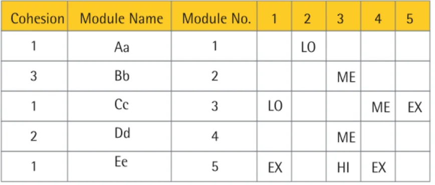
2. The no. of factors affecting the complexity within each of the modules Typical examples of an SCE input and output are given in Figures 2 and 3.
Figure 2: Typical SCE Input Cohesion Module Name
Aa LO ME ME HI ME EX EX EX LO Bb Cc Dd Ee Module No. 1 1 3 1 2 1 1 2 3 4 5 2 3 4 5
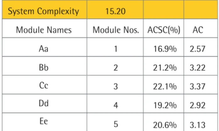
In Figure 3, the column ACSC(%) i.e. Application Contribution to System Complexity (%) is very important for test effort estimation purposes. This helps determine the distribution of effort across different modules. In the example shown, ACSC column suggests that we need 16.9 PDays to test the Module 'Aa' if the total test effort is 100 PDays.
While the SCE tool does not give a direct answer to the total effort required for testing, it gives a clear answer for distribution of effort among different modules. But, the 'System Complexity' information shown in Figure 3 can be used to estimate the total effort as well, provided we have the required inputs mentioned below. Scenario 1:
If we have the following information about a system which is similar to the SUT, we can arrive at an estimation of total effort required:
1) The system complexity of a second system (SC2) 2) The effort used for testing that system (EFF2)
Then the effort required for testing SUT, EFF1 = EFF2 * SC1/SC2 ; where SC1 is the system complexity of SUT.
Scenario 2:
In the event that we have several data points (System Complexity and Efforts) for a group of systems which are similar to SUT, we can derive a trend line using the following information.
The effort required for testing SUT, EFF1 = k * SC1
;where k is the proportionate ratio of 'Effort Vs Complexity' derived from the past data Analytical Hierarchy Program:
Another technique which can be used on similar lines is Analytical Hierarchy Program (AHP). This can be used in two circumstances:
1) As a second method for Effort Distribution Estimation along with SCE to reduce risk
2) When we do not have the complete system architecture knowledge; but only tacit knowledge which is sufficient enough to judge relative importance between modules taken two at a time
Figure 3: Typical SCE Output System Complexity
Module Names Module Nos. ACSC(%) AC 15.20 Bb Aa Cc Dd Ee 2 1 16.9% 2.57 21.2% 3.22 22.1% 3.37 19.2% 2.92 20.6% 3.13 3 4 5
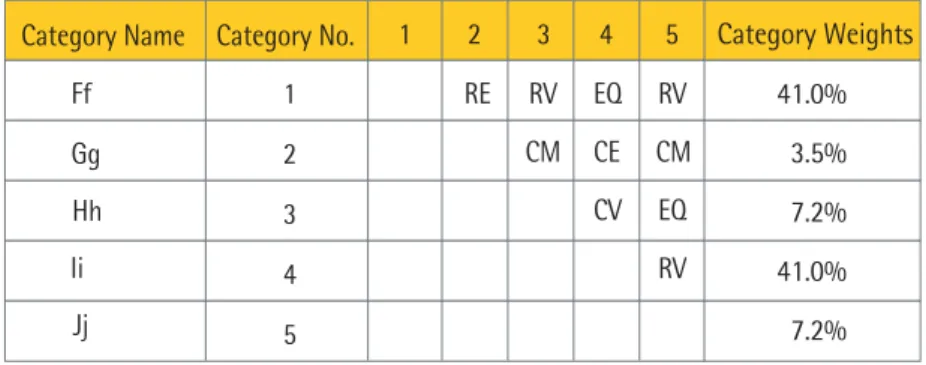
The input needed to apply this technique is only the relative importance of different modules of the system taken two at a time. AHP derives the relative importance of different modules from this pair-wise information.
Typical AHP input and output are given in Figures 4.
Figure 5 suggests that if the total system required 100 PDays of testing effort, module 'Hh' needs 7.2 PDays.
3. Test Sequencing
We have used module interdependency information in Phase 2 to derive system complexity. The same information, processed in a different manner can be used to determine the sequence between modules. This sequencing of information can be useful to schedule the testing activities in the Test Execution phase.
The tool used here is Dependency Structure Matrix (DSM). The input to the DSM is the Module interdependency information and the output is Module sequence for test execution. A typical input and output of the DSM tool is shown in Figures 6 and 7.
Figure 4: Typical AHP Input and Typical AHP Output
Figure 6: DSM Input Category Name Category No.
Gg Ff Hh Ii Jj 2 1 RE RV EQ RV CM CE CM CV EQ RV 1 2 3 4 5 3 4 5 41.0% 3.5% 7.2% 41.0% 7.2% Category Weights Module Nos. 2 1 1 1 1 1 1 2 3 4 5 3 4 5 Figure 7: DSM Output Levels 2 1 5 Modules -->> 3 3 4 2 1 4
As we can see in Figure 7, Modules 3 and 5 are at level 1. This means both these modules are to be tested first, before proceeding to the other modules. Module 4 is at level 2. This module has to be tested next before testing modules 2 and 1. This is good information to have since it helps us to prioritize between modules.
Also, it avoids unnecessary wastage of effort during test execution getting into re-testing mode because of dependencies. In the above example, Module 1 depends on Module 4. In the OUTPUT table, Module 4 is in level 2 and Module 1 is in level 4. This suggests that we have to test Module 4 before moving to Module 1. There is no meaning in testing Module 1 if we test and failed Module 4. Thus we save the effort of unnecessarily testing Module 1 in case Module 4 itself is not functioning rightly.
4. Test Suite Optimization
This phase is concerned with designing of test suite. The objective is to design a test suite which will maximize the test coverage and optimize the no. of test cases and the effort required.
Orthogonal Array (OA) is a technique to achieve this objective. This exercise starts with identifying the factors and levels of the system from the perspective of testing. Factors are defined as components of the system which work together to make the system itself. It can also be an attribute of the system. Levels are defined with respect to a factor. Levels are those values a factor can take at different points of time.
For e.g. in the case of a telephone network, the factors can be the originating party phone, line card, terminating party phone etc. The level of the originating party phone can be on-hook, off-hook etc. In the case of a GUI, a tab for entering SEX can be a factor. The levels are MALE and FEMALE for this factor.
With respect to the factors and levels defined above, using OA method, we can arrive at a particular set of combinations which together will satisfy the following two conditions:
1. All levels of all factors will have a presence in the set
2. All levels of a factor will appear against all levels of other factors at least Factor Name->
Sl. No.
2 1
FACA FACB FACC
3 a a a a a m n o p q m n o x y z w v y z w b b b 4 6 5 7 8 p v b 9 Factor Name-> Sl. No. 11 10
FACA FACB FACC
12 b c c c c q m n o p q m n x z w v x y w x c d d 13 15 14 16 17 o v d 18 Factor Name-> Sl. No. 20 19
FACA FACB FACC
21 d d a a a p q m n o p q y z v x y z w a a 22 24 23 25 Figure 8: OA Combinations
If we form test cases using the combinations suggested by OA, we will make sure of the following: 1. All states (values) of all components of the system are tested
2. All states of a component are tested against all states of other components at least once
This will make sure that we completely cover the system from a testing perceptive. This is achieved through a very minimum set of test cases. Let us take the following example. A system has three factors. Each of the three factors has got levels as follows:
Factor: FACA and Levels: a, b, c, d (Total levels = 4) Factor: FACB and Levels: m, n, o, p, q (Total levels = 5) Factor: FACC and Levels: v, w, x, y, z (Total levels = 5) The combinations given by OA are shown in Figure 8.
As we can see in Figure 8, OA gives 25 combinations which satisfy the rules described above. All the levels (i.e. a, b, p, x etc) of all factors are appearing at lease once. The level 'a' of FACA appears against the levels m, n, o, p and q of FACB at least once. The level 'a' appears against the levels v, w, x, y and z of FACC at least once. Similar is the case with other levels as well.
The full set of combinations possible in this example is 4*5*5 = 100. The no. of OA combinations is only 25. Here a saving of 75% can be seen in terms of no. of test cases. OA can be described as the best sample from the whole set of combinations from a testing perspective.
A practical example shows the following results: 1. Full set of combinations possible = 2400
2. No. of test cases used prior to OA implementation = 800 3. No. of test cases in OA Test Suite = 137
Here we can see a practical saving of 83% (reduction from 800 to 137) and a theoretical saving of 94% (reduction from 2400 to 137). Also, the testing can be at risk if the OA test cases are not a subset of the 800 test cases used earlier. This is because of test coverage issues.
In practice, practitioners are encouraged to add some more test cases to the OA test suite based on their experience. This is to avoid missing any important combinations to be tested from the experience they have. These test cases are called OA Complementary Coverage (OACC) test cases.
5. Resource Leveling And Scheduling
By now, we have test effort estimation and the test suite in place. The next thing is to arrive at a test execution schedule which can be used in the test execution phase. To determine the schedule, we should have the following inputs also:
1. Resource Vs. Module Matrix: This matrix gives the information on which resource can be used for testing which module
2. Resource Availability: This gives the information on which date a resource is available for testing activities 3. Modules Vs. Levels : This gives the information on which module is in which level (as detailed in the 'Test
Sequence' phase above)
4. Resource Weightage Matrix: This gives the information on the testing capability of each of the resource w.r.t. each of the modules
5. Maximum Resource: This gives the information on the maximum number of resources that can be used for a module at a time
6. Effort Vs. Module: Effort required for completing testing on each of the modules
Once these inputs are in place, we can do a resource leveling exercise and arrive at a possible schedule. A Resource Leveling Tool (RLT) can also be devised to generate a test schedule given the above inputs. If the schedule length (i.e. the total duration of test execution) we arrive at using Resource Leveling technique is more than the target duration, it means that more resources need to be added against some of the modules, which can be shortened. If the schedule is less than the target, we may examine the chance of pulling out some resources so that they can be used in other projects.
A typical RLT output is shown in Figure 9. Here M1,M2 etc are Modules and R1, R2 etc. are resources who will work on these modules. R1 shown in the cell (M1, 2) means that she works on Module M1 on the second day. There is no work assigned for R6 on the seventh day. This means that he can be released from the project after the sixth day.
Days--> Modules 1 2 3 4 5 6 7 M1 M2 M3 M4 R1, R3, R5 R2, R6 R2, R6 R2, R6 R1 R3, R5 R3, R5 R3, R5, R6 R3, R5, R6 R3, R5 R1 R1, R2 R1, R2 R1, R2 R2, R6 R1, R3, R5 Figure 9: RLT Output
There are three modes of testing which can be used in the test execution phase: 1) Testing by Suite 2) Testing by Exploration and 3) Testing by Pairs.
Testing by Suite
This is a straight forward method of testing as per the test cases decided by OA test suite. Test cases have to be divided between resources as per the output from the resource leveling phase.
Testing by Exploration
This is creative testing. A tester comes out of the conventional test suite scenarios and creates certain situations for the system and observes its behavior. This is a good way of forcing the system to break. In combination with OA test suite, this type of testing will ensure that the system is thoroughly tested. In projects where OA is used, the team gets a lot of time to do this type of testing and thus complements each other's effectiveness. This is because the OA test suite contains less no. of test cases than the conventional test pack.
Testing by Pairs
Testing by Suite is systematic method; Testing by Exploration is individual creativity. Testing by Pairs brings synergy among two testers and offers a chance for different ideas to complement each other and thus benefiting the final outcome.
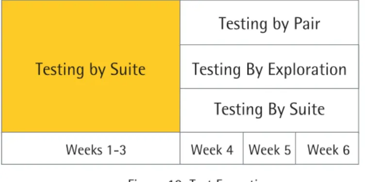
Figure 10 demonstrated how these testing modes can be used. In the example shown, during the first three weeks the team completes the Testing By Suite once. This way, the team can discover most of the defects early in the test cycle. In the next three weeks, team split their work between the three modes of testing. It is important to note that they repeat the Testing By Suite (partially or fully as required) to make sure that any bug fixes coming in is tested using the respective test cases.
Whichever testing method is used, we should have a Test Execution tracker.
6. Test Execution
Testing by Pair
Testing By Suite
Testing By Exploration
Testing by Suite
Week 4 Week 5 Week 6 Weeks 1-3
This will act as a log for testing. Ideally, a good test execution tracker will have the following fields among other things:
1. Version of system getting tested 2. Date of testing
3. Time stamp
4. Test case (Name / ID) 5. Tester
6. Status of test case (Pass, Fail, Hold, Abandoned)
Also important is how we analyze the defect trends and other metrics collected from the test bed / lab. Normally, we collect the following metrics from test bed. (Ref Figure 11)
1. No. of Test cases Executed 2. No. of Test Cases Passed 3. No. of Test Cases Failed 4. Test Effort
5. No. of Defects Reported 6. No. of Defects Rejected
We can have a tool called 'Defect Flow Analysis' (DFA), which comprehensively analyzes all these metrics and gives outputs. The advantages of having the same tool across different projects are:
1. Standard metrics analysis reports
2. Comparison between projects becomes easy
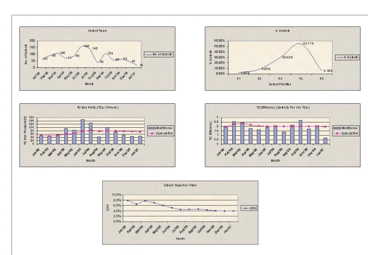
3. Reports come together with required graphs at once; thus comprehensive reports with less time The expected analysis reports from DFA are:
1. Defect Trend Report 2. Cumulative Defect Trend
3. Test Execution Productivity Trend 4. Test Case Efficiency Trend 5. Test Case Pass / Fail Rate 6. Defect Rejection Rate / Trend 7. Defect Severity Analysis etc.
All these reports are supported by required graphs for a better understanding by the manager. Refer Figure 12 for an example. The tool can also give a statistical summary of the trends in different individual reports.
Week Testing Effort(PDay) TCs executed TCs Passed No. of Defects Rejected Defects 1 2 3 4 83.75 56.13 102.13 74.56 903 731 1120 1033 757 683 721 824 34 25 32 27 0 1 0 2 Figure 11: Defect Report / Example
7. Defect Tracking And Closure
Defects will get reported once the test team begins the testing activity. These defects are to be tracked from the moment they are discovered till such time that they are fixed by the design team and retested by the test team. An ideal Defect Tracking tool should have among other things the following field entries:
1. Version of system 2. Date of testing 3. Test case (Name / ID) 4. Tester
5. Module impacted 6. Comments 7. Design contact
8. Status of defect (Raised, In Analysis, In Bug Fix, In Clarification, In Testing, Closed)
This defect tracking mechanism will be used by both testing and design teams. Ideally all the defects recorded in this system will have to be fixed and retested before a system can be released to field.
8. Reliability Estimation And Release
There are several factors which help us decide when we can release a product to field. One of the important factors is Residual Defect Estimation. Residual defects are those defects which have not been discovered yet, even after a certain amount of testing activity.
We can have a Residual Defect Estimator which analyses the trend of the defects detected over a period of time through out the testing cycle. The input to this estimator is the Defect Report which is mentioned in the phase 'Test Execution'. The outputs from this trend analysis are:
1. The estimated count of residual defects; and
2. The estimated time for testing to discover the residual defects
Suppose in as typical project, after analyzing the defect trends, the tool estimates that there are still 25 defects in the system out of 600 estimated total defects, tt suggests that 4% defects are still in the system which are yet to be discovered. There are two questions asked at this point:
1. With 4% residual defects (25 nos), can we stop testing and release the product to the field?
2. If the answer is No, how much more effort do we need to spend further on testing to discover these defects (an estimation)? If this estimation is found to be reasonable, the manager can continue testing. If the effort is huge, the manager may decide against further testing after considering parameters in SLA (Service Level Agreement) and other criteria.
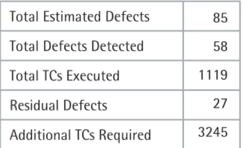
Figure 13 shows an output from a typical Reliability Estimation exercise. In the example shown, total estimated defects in the system are 85 and residual defects are 27. It also estimates that 3245 test cases (or equivalent effort) are required to discover the residual defects.
9. Maintenance Testing
During the maintenance phase of a system, there will be defects reported from the field and Change Requests (CRs) will be raised. This leads to further enhancement of the system and the system needs to be tested again. Here, there is a need to find out how much time one needs to spend testing a particular module or a CR relatively. This is to make sure that the valuable test effort is distributed appropriately across different modules and CRs. A technique called System Change Impact Matrix (SCIM) can be used to determine this distribution of effort.
Total Estimated Defects Total Defects Detected Total TCs Executed Residual Defects Additional TCs Required 85 58 1119 27 3245 Figure 13: Typical Reliability Estimation Output
The inputs needed are:
1. The system complexity of the system
2. The relative complexity of each of the modules
3. The impact of each of the CRs on each of the modules on a one-on-one basis (if any)
The first two inputs come directly from Test Phase 2: System Study and Estimation. The third information is to be determined after analyzing each of the CRs. The outputs of System Change Impact analysis will be:
1. Change impact index
2. Relative impact on each of the modules 3. Relative impact of each of the CRs
The output 2 can be used to determine in what way the total test effort has to be distributed across different modules. The output 3 can be used to determine how much of the test effort has to be spent on each of the CRs. This leads to proper selection of test cases covering all modules and CRs appropriately.
A typical analysis output of a SCIM is shown in Figure 14. This example suggests that the team has to spend 29% of the test effort on CR no. 3 and 17% on Module 4 and so on. This also suggests that Module 1 is not impacted at all and the test manager can decide whether he can avoid testing this module based on priorities.
Change Impact Analysis
1. CR Impact Analysis
2. Module Impact Analysis
Change Impact Index
CR Nos. Mdl Nos. 1 2 3 4 1 2 3 4 5 6 7 8 0% 20% 8% 17% 14% 21% 7% 13% 0.00 4.03 1.58 3.47 2.81 4.21 1.33 2.58 14% 15% 29% 41% 2.86 3.03 5.87 8.24 %FII FII %MII MII 23.92
Conclusion
The test phases, techniques and tools described in this article together draw a systematic picture of the whole test cycle.
1. VoC helps to capture requirements correctly and without ambiguity so that we can have the information on what to look for while doing testing. RTM is used to track the requirements till the testing cycle is completed. 2. Effort estimation and distribution techniques help to know the relative complexity between modules so that
the testing team can split their effort between modules accordingly.
3. DSM helps to sequence the testing of different modules so that the execution plan is proper, thus avoiding any unnecessary and avoidable delays.
4. OA technique helps to maximize the test coverage and optimize the test suite.
5. Resource leveling techniques ensure that we have the optimum schedule as per the resource availability and capability. It also plans for resource movement across modules as per their expertise.
6. The 3 modes of test execution are 1) Testing by Suite 2) Testing by Exploration and 3) Testing by Pairs. This ensures that the system is tested on 360 degrees basis. DFA is used to analyze all the metrics which are collected from Test Bed.
7. Defect Tracking Mechanism ensures that the bugs are tracked properly till they get fixed and retested. 8. Reliability estimation predicts the residual defects in the system so that the test manager can take the
decision to continue or to stop testing accordingly.
9. System Change Impact Matrix helps us to determine the relative effort distribution between modules and CRs during maintenance testing.
Gaining knowledge of these tools and techniques is important for a test manager. The latter also has to apply there tools religiously in the project to achieve the objective of better testing with minimum or optimized effort.
References
1. Six Sigma DMAIC Training documents, Wipro Technologies, Internal Publication, 2005
2. Bhushan Navneet and Rai K., Strategic Decision Making - Applying the Analytic Hierarchy Process, Decision Engineering Series, Springer, UK, Jan 2004.
3. Bhushan Navneet, System Complexity Estimator, Productivity Office, Wipro Technologies, Internal publication, Dec 2004
4. Bhushan Navneet, System Change Impact Model, Productivity Office, Wipro Technologies, Internal publication, Aug 2005
5. Bhushan Navneet, Deploying Paired Programming, Productivity Office, Wipro Technologies, Internal Publication, 2005
6. Arunachalam Ganesh, Varma Pramod, TN Ajikumar, Robust Testing Methodologies , Wipro Technologies, Internal Publication, 2005
7. Arunachalam Ganesh, Varma Pramod, TN Ajikumar, Guidelines to Reliability Measurement , Wipro Technologies, Internal Publication, 2005
About The Author
Ajikumar TN is at present 'Head-Testing Competency Team' in the Testing Services Division of Wipro Technologies, Bangalore. He holds an MBA in Software Enterprises Management from Indian Institute of Management, Bangalore and a B Tech Degree in Electronics & Communication Engineering. He has got about 12 years of experience in the software industry and has worked for enterprises like BPL Telecom earlier. He can be reached at [email protected].