Globalisation and the euro area: simulation based analysis using the New Area Wide Model

Working PaPer SerieS

no 907 / June 2008

globaliSation and

the euro area

Simulation baSed

analySiS uSing

the neW area

Wide model

WO R K I N G PA P E R S E R I E S

N O 9 0 7 / J U N E 2 0 0 8

In 2008 all ECB publications feature a motif taken from the 10 banknote.

GLOBALISATION AND THE EURO AREA

SIMULATION BASED ANALYSIS USING

THE NEW AREA WIDE MODEL

by Pascal Jacquinot

_{and Roland Straub}

This paper can be downloaded without charge from http://www.ecb.europa.eu or from the Social Science Research Network electronic librar y at http://ssrn.com/abstract_id=1138607.

© European Central Bank, 2008 Address

Kaiserstrasse 29

60311 Frankfurt am Main, Germany

Postal address

Postfach 16 03 19

60066 Frankfurt am Main, Germany

Telephone +49 69 1344 0 Website http://www.ecb.europa.eu Fax +49 69 1344 6000

All rights reserved.

Any reproduction, publication and reprint in the form of a different publication, whether printed or produced electronically, in whole or in part, is permitted only with the explicit written authorisation of the ECB or the author(s).

The views expressed in this paper do not necessarily refl ect those of the European Central Bank.

The statement of purpose for the ECB Working Paper Series is available from

Abstract 4 Non-technical summary 5 1 Introduction 8 2 The framework 10 2.1 The model 11 3 Model calibration 13 3.1 Domestic dimension 13 3.2 International dimension 14 4 How to measure the impact of globalisation on

the euro area? 15 4.1 Model-based defi niton of globalisation 16 4.2 Identifying the channels of transmission 17

4.2.1 The increase of potential output in emerging Asia 18 4.2.2 An increase in openness in the euro

area 19

4.3 Globalisation scenarios 20 5 Transitional dynamics 22 6 Structural reforms in the euro area

and globalisation 23 7 Conclusion 24 References 25 Appendix A 26 Appendix B 33 Appendix C 36

European Central Bank Working Paper Series 40

CONTENT S

Abstract

In this paper, we utilise the multi-country version of the NAWM to analyse the impact of globalisation on euro area macroeconomic aggregates. We provide alternative model-based definitions of globalisation associated with an increase in potential output in emerging Asia and its impact on total factor productivity in the euro area, and a shift in international specialisation patterns leading to changes in relative demand and import substitutions. The results indicate that globalisation has a positive impact on output, consumption, investment and real labour income in the long-run. This impact is driven by the improvement in the terms of trade and associated positive wealth effects, as well as by spillovers of higher potential output in emerging Asia on euro area total factor productivity. Additionally, we provide evidence that structural reforms in goods and labour markets would amplify the benefits associated with globalisation.

Keywords: DSGE modelling, globalisation, euro area JEL Classification: E32, E62

Non-technical Summary

In this paper, we argue that globalisation contributes to improve standards of living in the euro area due to the benefits arising from trade with emerging economies. For demonstrating the channels through which globalisation is potentially affecting the euro area, we utilise the recently developed multi-country version of the New Area Wide Model (NAWM). The multi-country version of the NAWM is an open economy dynamic stochastic general equilibrium model (DSGE) calibrated to represent the euro area, United States, emerging Asia, and a remaining countries bloc, respectively.

In the model set up, we define globalisation as an increase in potential output in emerging Asia driven by an increase in total factor productivity and in the rise in the pool of labour force. We also provide some assessment on the impact of a change in comparative advantage pattern in the world.

The wealth created by the increase in potential output are transferred to the euro area via trade in goods. The euro area economy is impacted by the increase in potential output in emerging Asia through (i) a terms-of-trade effect, as goods imported from these economies become cheaper; (ii) a substitution effect, as euro area firms are then induced to pro-duce more efficiently, by substituting cheaper intermediate goods imported from emerging economies to domestic intermediate goods; (iii) a wealth effect, as euro area consumption and investment both increase due to availability of cheaper goods; (iv) in addition, the wealth effect allows to work less for a given level of desired consumption and leads to an increase in leisure.

For instance, assuming that globalisation leads to an increase in output in emerging Asia of 40 percent in the long-run (of which four-fifths is due to higher productivity and the rest to an increase in the available pool of labour), we show that output, consumption and investment in the euro area would also increase by more than 2 percent in the long run, while real wages would rise by more than 3 percent and leisure by close to 1 percent. The benefits from globalisation for the euro are compounded with strong productivity spillovers from the emerging market world.

devel-opment in emerging Asia relies less on productivity and more on increasing labour force participation. For instance, assuming that a 1 percent increase in productivity in emerging Asia brings a 0.05 percent increase in productivity in the euro area, a similar increase in output in emerging Asia of 40 percent as under the previous scenario, but based on opposite development patterns (one-fifth due to higher productivity and four-fifths due to an increase in the pool of labour available) would lead to a much smaller gain in euro area output in the long-run (0.3 percent). Likewise, the increase in consumption, investment and real wages would be more limited (around 1 percent). The latter result is driven by the assumption that labour supply driven developments strategy dampens the productivity spillover to the euro area.

Furthermore, we argue that a key challenge for the euro area is also to ensure that it does not lose its competitive edge relative to emerging economies, which would then somewhat dampen the benefits from globalisation. A common concern is that increasing competitive-ness and rising quality of goods produced in emerging economies could ultimately lead to a complete shift in euro area consumption away from domestic goods, including for those goods for which euro area producers had a competitive edge thus far. Such an increase in euro area demand for emerging economy goods would lead to: (i) an increase in euro area import prices, and thereby to deterioration in the terms of trade and to a fall in real wages; (ii) in equilibrium, as a result of the deterioration of the terms of trade, to a substitution ef-fect towards euro area goods and away from emerging market goods; (iii) an adverse wealth effect and a fall in real consumption, with a given level of desired consumption requiring a reduction in leisure and longer working hours. For instance, assuming that emerging Asian firms start to produce goods previously produced in the euro area only and that the euro area’s imports-to-GDP ratio increases by 2 percent, our simulations suggest that leisure would fall by 0.2 percent, real consumption by 0.5 percent and real wages by close to 1 percent in the long run. The increase in working hours would lead to an increase in euro area output of 0.2 percent, however.

Furthermore, we argue that structural reforms can contribute to maximise the benefits from globalisation, but sequencing is important to address potentially adverse impacts on

labour markets, notably on wages. Reforms in goods markets, which are associated with stronger competition among firms and with a reduction in mark-ups, can compound the positive effects of globalisation. For instance, assuming that such reforms lead to a reduction in goods mark-ups from 15 percent to 5 percent, output increases by 10 percent in the long run - relative to a scenario taking into account globalisation effects solely - as firm are less able to take advantage of their market power. Likewise, real consumption rises by another 3 percent and real wages by a further 20 percent. Reforms in labour markets lead to similar results, with the exception of the real wage impact, as the ability of workers to exploit their market power is lessened. For instance assuming a reduction in wage mark-ups from 25 percent to 15 percent, such reforms would lead to an increase in output by a further 3 percent, as well as to an increase in real consumption by another 3 percent. Conversely, the increase in real wages would fall short of 0.5 percent, relative to a scenario taking into account globalisation effects solely.

1

Introduction

Globalisation is a widely used term in policy debates. Although, there are certainly different dimensions of globalisation, such as the increase in cultural and political linkages between different regions in the world, the term is usually used in context of ”economic globalisa-tion”. There are several attempts to characterise and define economic globalisation. Wolf (2004), for example, associate globalisation with the ”movement in the direction of greater integration, as both natural and manmade barriers to international economic exchange continue to fall”. Bernanke (2006) acknowledge that trade between countries has been in-creasing intermittently in the last centuries, but ”(t)he emergence of China, India, and the former communist bloc countries implies that the greater part of the earth’s population is now engaged, at least potentially, in the global economy.” This dramatic intensification of the globalisation process is transforming the economic structures of the developed and developing world. This goes in line with the reduction of trade barriers and home bias in goods and asset markets, which are reflected by an increasing share of imported goods in the global production process and the rise of cross-border holdings of financial assets in the global economy. As a result, economic globalisation, defined above, can be considered as the largest structural upheaval since the industrial revolution.

In order to give an indication of the rapid pace of developments, we present in Figure 1 the evolution of labour productivity and labour force in China in the previous years. Since 1988, labour productivity in China has increased by more than 150 percent, while the labour force by over 20 percent. These developments are also reflected in the very high average real GDP growth rate in China. Interestingly, the last decade of the previous century were contemporaneously associated by a substantial decline in average tariff rates in the European Union (see lower-left panel of Figure 1). As a result, it is natural to ask how the described developments, which we associate in broader sense with globalisation are likely to affect macroeconomic aggregates in the long-run.

The literature on the effects of real globalisation, i.e. abstracting from the effect of increasing financial integration, on macro aggregates has risen substantially in the recent years. The most comprehensive study so far on the effects of globalisation on Europe has

been produced by the European Commission (Denis, Mc Morrow and R¨oger, 2006). The academic literature has so far focused mainly on the impact of globalisation on inflation. See for example contributions by Rogoff (2003), or Kamin, Marazzi and Schindler (2006). Chen, Imbs and Scott (2004) argue, using a disaggregated data set for EU manufacturing sectors, that productivity and markup effects, driven by the increase in market shares of low-cost emerging economies, are significant and have equally important impact on euro area macro variables in the short term, whereas the effects of productivity is dominating in the long run.

This paper aims to look at the issue of globalisation through the lens of a dynamic stochastic general equilibrium model. There are various advantages of using macro-models, when analysing such a complex phenomena as globalisation. First and most importantly, in a general equilibrium models the inter-linkages between the different variables provide an important feedback mechanism that is lacking in a partial framework. In addition, in econometric analysis it is difficult to control for all possible shocks affecting historical data and consequently to measure a ”pure” effect of a shock. In a model, however it is possible to single out structural shocks, which allow for the identification of independent channels and mechanisms. In this way the impact of globalisation can be disentangled into opposing forces with identified signs and sizes even when net effects are hard to measure. Therefore, in a model framework, assumptions are easier to monitor and transmission mechanisms are easier to identify than in empirical exercise.

Therefore, in this paper, we utilise the multi-country version of the New Area Wide Model (NAWM), recently developed in Jacquinot and Straub (2007) for analysing the im-pact of globalisation on the euro area. Furthermore, we provide a model-based definition of globalisation, identify the channels through which globalisation is affecting macro aggre-gates, and provide some quantitative analysis of the potential impact of globalisation on the euro area.

The paper is organised as follows. Section 2 discusses in a nutshell the features of the multi-country version of NAWM. Section 3 presents the calibration of the model. Section 4 provides a set of model-based definitions of globalisation and the corresponding impact of

1990 1995 2000 100 150 200 250 Productivity in China 1990 1995 2000 100 105 110 115 120

Labour Force in China

19802 1985 1990 1995 2000 2005 4 6 8 10 12 14 16 Real GDP China 1990 1995 2000 5 10 15 20 25 30 35 40

Average Tariffs in the EU

Figure 1: Productivity (defined as valued added divided by labour force), real GDP growth and labour force data in China is calculated using data from the World Development In-dicators (WDI) data base of the World Bank. Productivity and Labour Force is an index with the base year 1988. The average tariff data is from the Fraser Institute.

the latter on euro area aggregates. Section 5 discusses the transitional dynamics following the structural changes/ shocks triggered by the process of globalisation, while section 6 assesses whether structural reforms in goods and labour markets are able to amplify the effects associated with globalisation. Section 7 concludes.

2

The Framework

In the following sections, we outline the features of the multi-country version of the NAWM model, as discussed in Jacquinot and Straub (2007) and present the calibration of the model. We provide a detailed description of key parts of the model in Appendix A. The reader that is not interested in modelling details can skip these section and can move immediately to section 4.

2.1 The Model

The multi-country version of the NAWM builds on recent advances in developing micro-founded Dynamic Stochastic General Equilibrium (DSGE) models suitable for quantitative policy analysis, as exemplified by the closed-economy model of the euro area by Smets and Wouters (2003), the International Monetary Fund’s Global Economy Model (GEM; cf. Bayoumi, Laxton and Pesenti, 2004), the Federal Reserve Board’s new open economy model named SIGMA (cf. Erceg, Guerrieri and Gust, 2005), and the two-country version of NAWM as discussed in Coenen, McAdam and Straub (2007). Thus, it incorporates a relatively large number of nominal and real frictions in an effort to improve its empirical fit regarding both the domestic and the international dimension.

The multi-country version of the NAWM consists of four symmetric countries of different size representing the euro area (EA), United States (US), emerging Asia (EM), and a remaining countries (RW) block respectively. International linkages arise from the trade of goods and international assets, allowing for imperfect exchange-rate pass-through to consumer prices and imperfect risk sharing. In each country, there are four types of economic agents: households, firms, a fiscal and a monetary authority. Extending the setup in Coenen and Straub (2005), the NAWM features two distinct types of households which differ with respect to their ability to participate in asset markets, with one type of household only holding money as opposed to also trading bonds and accumulating physical capital. As a result, also households with limited ability to access asset markets can intertemporally smooth consumption by adjusting their holdings of money. Due to the existence of these two types of households, fiscal policies other than government spending—notably transfers— also have real effects even though both types of households are optimizing consumption and labour supply subject to intertemporal budget constraints. Further, it is assumed that both types of households supply differentiated labour services and act as wage setters in monopolistically competitive markets by charging a markup over their marginal rate of substitution. Specifically, wage setting is characterised by sticky nominal wages and indexation, eventually resulting in two separate wage Phillips curves. Moreover, in order

to establish a more pronounced role of transfer payments made by the fiscal authority, we assume that transfers, in per-capita terms, are unevenly distributed across the two types of households, favouring the constrained households with limited asset-market participation over the unconstrained ones in a proportion of three to one. This also helps to guarantee that the levels of consumption and hours worked are not too dissimilar across households.

Regarding firms, the NAWM distinguishes between producers of tradable and nontrad-able differentiated intermediate goods and producers of three non-tradnontrad-able final goods: a private consumption good, a private investment good, and a public consumption good. Fi-nal good producers in the consumption good and investment good sector utilize imported intermediate goods in their production process 1, while public consumption good is only consuming goods of domestic origin. Domestic tradable and nontradable intermediate-good producers sell their differentiated outputs under monopolistic competition, while the final-good producers operate under perfect competition and take prices as given. In the tradable and nontradable intermediate good sector, there is sluggish price adjustment due to staggered price contracts and indexation, yielding two separate price Phillips curves.

The fiscal authority purchases units of the public consumption good and makes transfer payments to the two types of households, in unevenly distributed amounts. These expenses are financed by different types of distortionary taxes, including taxes on consumption spend-ing, labour and capital income, as well as profits. A simple feedback rule is assumed to stabilize the government debt-to-output ratio by appropriately adjusting a suitable fiscal instrument.

Finally, the monetary authority is assumed to follow in all economies but emerging Asia, an inertial Taylor-type interest-rate rule with interest-rate smoothing, which is specified in terms of annual consumer-price inflation and quarterly output growth. In emerging Asia the monetary authority is assumed to follow a fixed exchange rate regime.

1_{Imported intermediate goods are a CES aggregate of imported intermediate goods from different regions.}

For example, the euro area imported intermediate good is an aggregate of US, emerging Asia and remaining countries imported goods, see Jacquinot and Straub (2007) for details

3

Model Calibration

The parametrisation of the model draws heavily on the results of estimated DSGE models such as Smets and Wouters (2003), Christiano, Eichenbaum and Evans (2005), and on the former version of the NAWM described in Coenen, McAdam and Straub (2007). With regards to the international dimension, the model utilises estimated values reported by de Walque, Smets, and Wouters (2005). In what follows, we highlight the differences to Coenen, McAdam and Straub (2007) with particular emphasis on the calibration of the international dimension.

3.1 Domestic Dimension

In Appendix B, Tables A through E document the parametrisation adopted for the four regional blocs. Unless otherwise stated, similar behavioral parameter values apply to all regions. First, Table A presents the main macroeconomic aggregates of the different regions calibrated to match stylized facts in the data. Table B depicts the parameters that are key for the consumers’ optimization problem. Although consumers may differ with respect to their access to financing, the preferences of the liquidity-constrained and forward-looking households are taken to be the same. We assume that in US, euro area and in the remaining countries block, the share of liquidity-constrained consumers is 25 percent. The share is much higher in emerging Asia at 50 percent, reflecting the underdeveloped financial markets for domestic consumers. The rate of time preference is in the current version of the model is assumed to be equal around 0.993 in all regions. The intertemporal substitution in consumption set at 0.5. The value of habit persistence equals 0.6. Conversely for labour, we assume that the inverse of the Frisch leasticity of labour supply is 2. The values are taken from the previous version of the NAWM, and are not updated given the lack of information on the size of these parameters for the regions of interest. Furthermore, we assume for both households a Calvo parameter determining the persistence of wage adjustment of 0.75, roughly equivalent to a four-quarter contract length under Calvo-style pricing. Similarly, in the labour market households have pricing power, resulting in the wage markups. For US and the euro area markups (16 percent and 30 percent respectively) correspond to Bayoumi,

Laxton and Pesenti (2004). We further assume that RW is somewhere in between US and euro area, with a 20 percent wage markup, while we assume EM has a labour market as competitive as the US. In the production sector, the bias towards the use of capital in both sectors is calibrated to achieve a relatively high investment share of GDP in EM, and a low share in US, in line with their respective historical averages. The calibration can be done by adjusting tax rates or the technology parameter, currently we decided to choose the former, leaving the technology parameter α at 0.3. The depreciation rate is assumed to be 2.5 percent per quarter across all regions. Real rigidities in investment and import adjustment costs align with the parametrization of the baseline NAWM. The estimates for the price markups are taken from Martins, Scarpetta and Pilat (1996). The US bloc has the lowest price markups, indicating the greatest degree of competition, while euro area have the highest. Finally, to provide a nominal anchor for the domestic economy, monetary policy is parameterized as follows. US, euro area and remaning countries block follow an Taylor rule with the calibration borrowed from the baseline NAWM. Emerging Asia is assumed to pursue a fixed exchange rate regime against the US dollar.

3.2 International Dimension

The main results of the model rely heavily upon the calibration of each region’s external sector in Table G. For given steady-state net foreign asset positions for each region, it is straightforward to calculate the current account and trade balances consistent with long-term stock-flow equilibrium. Using the IMF’s Direction of Trade Statistics on merchandise trade, the national accounts data on the imports of goods and services, and the United Nations’ Commodity Trade Statistics (COMTRADE) data on each region’s imports of con-sumer and capital goods, we derive a disaggregated steady-state matrix delineating the pattern and composition of trade for all regions’ exports and imports. On the basis of this trade matrix, we derive all the weight coefficients in the demand function for imports and the regional composition of imports (see Table D). For the corresponding trade elasticities, we assume that the elasticity of substitution between domestically-produced and imported tradable consumption goods and investment goods is 2.5. The elasticity of substitution between goods from different regions for imported consumption goods and imported

invest-ment goods is set at 1.5, consistent with existing estimates of import elasticities. Lastly, we need to calibrate the behavior of net foreign assets. For the long-run behavior of net foreign assets our prior is that a permanent increase in government debt by one percentage point of GDP is roughly associated with an increase in the net foreign liability position of the region by 0.5 percentage points of GDP2. Moreover, when the US expands its net foreign liabilities as a result of a permanent change in its public debt, the absorption of new issuance by each region is calibrated (on the basis of net foreign asset holdings in recent years) by assigning 24 percent of new issuance by US to emerging Asia, and 38 percent to each of euro area and remaining countries. This calibration implies that for a one percent net foreign liabilities to GDP shock in the US, the emerging Asia’s net-foreign-asset-to-GDP rises the most — around 0.8 percent of GDP — while euro area and the remaining countries see their ratios only rise by around 0.3 and 0.5 percent of GDP respectively.

4

How to Measure the Impact of Globalisation on the Euro

Area?

As discussed above, we associate globalisation with three main driving factors: (1) increase in productivity and (2) labour supply in emerging Asia and (3) reduction in trade barriers in the industrialised world. While the first two capture one specific aspect of globalisa-tion, namely the increase in potential output in emerging Asia, the latter represents the reduction of institutional and technological constraints in the euro area, which has triggered an increase in demand for goods originating in the rest of the world 3. Alternatively, the reduction in home bias could also be interpreted as changes in international specialisation patterns inducing a shift in relative demand of domestically produced goods. With that in mind, we provide in this section a model-based analysis on the impact of globalisation on the euro area in a multi-country version of the New Area Wide Model (NAWM). The results of the scenario analysis are presented in Appendix C.

2_{Overlapping generations models (particularly those which follow the Blanchard-Weil-Yaari formulation)}

provide theoretical underpinnings to evaluate this non-Ricardian behavior.

3_{In the model, the increasing demand for goods associated with the decrease in home bias is captured at}

the firm level. One could easily argue that the reduction of trade barriers and technological constraints also lead to an increase in final good consumption from emerging Asia. In our model, however, trade integration

4.1 Model-Based Definiton of Globalisation

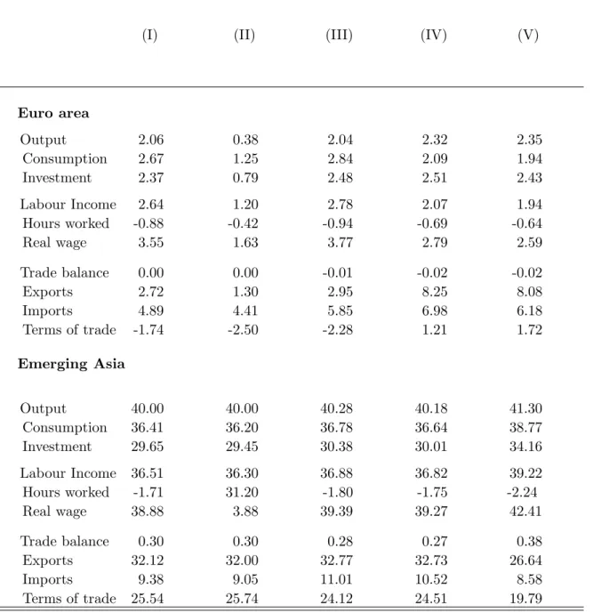
First, we provide a model-based definition of globalisation in terms of quantifiable shocks hitting the world economy. Furthermore, given differing views on the nature of globalisation, we will also discuss in this section four alternative ”economic globalisation” scenarios.

In scenario (I), the benchmark simulation, we assume that globalisation is associated with a 40 percent long-run increase in GDP in emerging Asia. The increase in GDP is calibrated in such a way that 80 percent of the increase is due to a rise in total factor productivity and 20 percent due to an increase in labour supply in emerging Asia. The increase in productivity in emerging Asia is assumed to have spillovers to euro area total factor productivity (TFP). In particular, a 1 percent increase in emerging Asia TFP has a 0.05 percent impact on TFP in the euro area. We argue that globalisation is closely associated with technological spillovers, with significant implications for productivity, in-cluding: (i) direct technology transfer, through imports of capital goods (ii) economies of scale effects, notably the possibility for firms to increase the scale of their operations; (iii) ”defensive” innovation, with firms becoming more innovative in response to stronger com-petitive pressures globally. In this context, the magnitude of the gains for the euro area from globalisation also depends on the extent of the productivity spillovers from emerging economies.

Note that according to the latter scenario, the increase in GDP in emerging Asia does not necessarily induce a fundamental change in the production structure in the euro area. While the technological progress in emerging Asia induces a relative price (terms of trade) effect, it does not trigger an increase in the quasi-share of foreign goods (a reduction in home bias) in production in the long-run. In other words, the increase in TFP and labour supply in emerging Asia does not lead to a shift in demand in favour of emerging Asia goods, beyond the effect induced by the change in the terms of trade.

In scenario (II), we assume that the labour supply shock plays a more prominent role in driving the 40 percent increase in output in emerging Asia. As the role of productivity is dampened, the spillover to euro area TFP are also subdued.

Scenario (III) is similar to scenario (I), but we assume that the euro area is lagging behind the US and the remaining regions in benefiting from the positive (TFP) spillovers associated with globalisation. In particular, we assume that the spillovers from emerging Asia to the US, and the rest of the world block are twice as strong as to the euro area.

In scenario (IV), we assume that the technological progress in emerging Asia is also associated with a contemporaneous reduction in home bias in the euro area. A possible explanation for this could be that the technological progress in emerging Asia allows for production of goods and services, which were previously produced only in the euro area, inducing changes in international specialisation patterns. The latter in isolation leads to a change in relative demand in the euro area with its corresponding impact on relative prices

4_.

In scenario (V), we push the previous argument further assuming that the technological progress in emerging Asia does not only lead to a shift in relative demand in the euro area, but also to an import substitution effect in emerging Asia (increase in home bias).

4.2 Identifying the Channels of Transmission

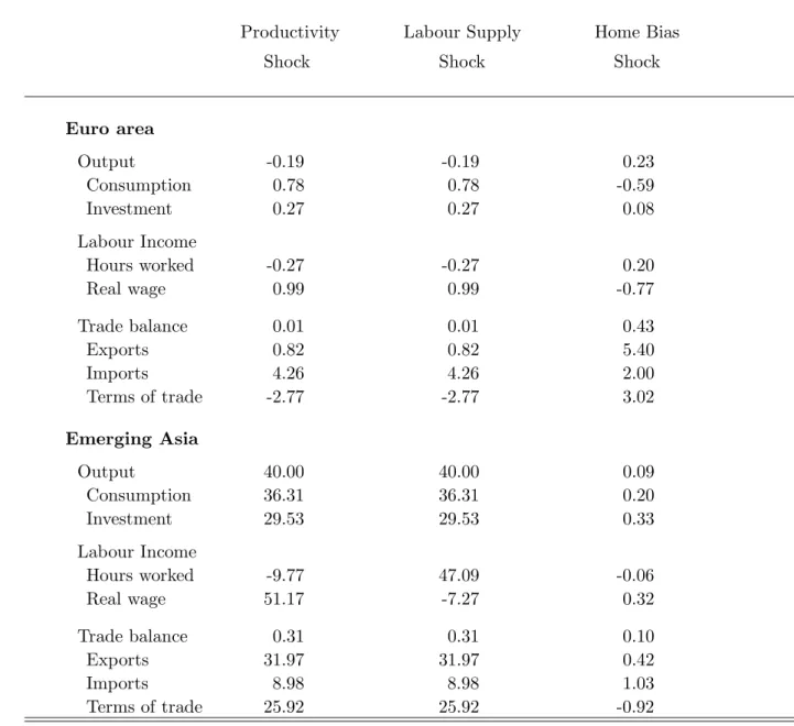
Before turning to the analysis of the various scenarios, it is helpful to analyse the effects of the individual shocks in our model. The latter will help us to understand and to identify the channels through which economic globalisation is affecting macroeconomic aggregates. As a result, we first show separately the effects of productivity and labour supply shocks in emerging Asia, and the impact of a reduction in home bias in the euro area on macro aggregates, before presenting the results of the discussed globalisation scenarios. Total factor productivity and labour supply shocks are calibrated to generate a 40 percent increase in GDP in emerging Asia, while the home bias shock to trigger a 2 percent increase in the import to GDP ratio in the euro area. The results in Table 1 are presented as percentage changes compared to the old steady state of the model.

4_{Alternatively, one could see the fall in home bias, as a reduction in institutional constraints/non-tariff}

4.2.1 The Increase of Potential Output in Emerging Asia

The permanent increase in productivity has a substantial positive impact on consumption and investment in emerging Asia. At the same time, the rise in total factor productivity reduces hours worked in the long-run through the generated positive wealth effect 5. The relative increase in the supply of goods from emerging Asia leads to a deterioration of the terms of trade (defined as the relative price of imports to exports) in emerging Asia, and a corresponding improvement in the terms of trade in the euro area. The improvement of the terms of trade in the euro area has three main effects in the long-run: (1) a pos-itive wealth effect associated with the terms of trade improvement, which has a pospos-itive impact on consumption and investment; (2) a reduction in hours worked due to the positive wealth effect; (3) a substitution effect due to the relative decrease in the price of goods from emerging Asia, which induces euro area tradable firms to substitute away from domestic to foreign tradable intermediate goods. The latter two factors imply jointly a slightly negative long-run impact on euro area GDP (-0.19 percent compared to the old steady-state). Note, however, that using a model based welfare function (the utility of the households in the model), welfare in the new steady state appears to be higher, as both consumption and leisure increases compared to the old steady-state. In conclusion, while a positive produc-tivity in emerging Asia could have a slightly negative impact on euro area GDP, it leads to overall welfare improvement in particular due to the rise in purchasing power triggered by the improvement in the terms of trade.

Permanent labour supply shock in emerging Asia has the same effect on euro area aggregates, but induces significantly different impact on real wages in emerging Asia. The similar impact of labour supply shock and productivity shocks on the euro area is not surprising as they both affect the long-run potential output in the same way. In fact, note that while real wages react differently in the model, the real income of households (product of real wage and hours worked) are very similar under both scenarios6.

5_{In this type of models an increase in hours worked usually indicates the existence of a negative wealth}

effect on households. Note also that the model-based welfare measure depends positively on consumption and leisure. As a result, and in contrast to the ”conventional view”, a decrease in hours worked is associated with a rise in welfare in the model.

4.2.2 An Increase in Openness in the Euro Area

A reduction in the home bias parametersϑCandϑI, defined in details below, has a

substan-tially different impact on the euro area in our simulation exercise. The home bias parameter determines the share of imported goods in the final production of tradable consumption and investment goods for a given elasticity of substitution. In particular, considering only the consumption sector, the bundle of tradable goodsT_tC is produced by the following constant elasticity of substitution technology:

TtC = ⎛ ⎜ ⎝ϑ 1 μC_T C HtC 1− 1 μC_T + (1−ϑC) 1 μC_{T (1−Γ} IMC(IM_tC/QC_t ))IM_tC 1− 1 μC_T ⎞ ⎟ ⎠ μC_T μC_T−1 (1)

whereHtC is a bundle of domestic produced tradable andIMtC is bundle of imported tradable

goods,μC_T stands for the intratemporal elasticity of substitution between the distinct bundles of tradable domestic and imported goods, andϑC determines the share of domestic tradable

goods compared to imported goods. Notice that the consumption-good firm incurs a cost, Γ_IMC(IM_tC/QC_t ), when varying the use of the bundle of imported goods in producing the tradable consumption good. The corresponding demand functions for IM_tC is defined as follows: IM_tC = (1−ϑC) PC IM,t PC T,tΓ†_{IMC,t −μ}C T TC t 1−Γ_IMC(IMC t /QCt), (2)

where P_T,tC , P_IM,tC are the corresponding prices of inputs, while Γ†_IMC_,t = 1 − Γ_IMC(IM_tC/QC_t )−Γ_IM C(IM_tC/QC_t )IM_tC represents the first order derivative of the import adjustment cost functions. Note that in the steady state the adjustment cost of imports equals to zero, while the first derivative of import adjustment costs is one. Consequently, in the steady state (1−ϑC) determines the share of domestic tradable goods for a given

value of elasticity of substitution, or jointly with the corresponding parameter in the invest-ment sector (1−ϑI), the openness of the economy. Correspondingly,ϑC andϑI determines

emerging Asia, particularly in China have remained relatively stable despite the rise in productivity. In particular, the migration of an increasing number of workers from central China to the dynamic coastal

the degree of home bias in the model. Home bias can be interpreted as a technological constraint for a firm, determining the relative response of imported goods following an ex-ogenous increase in the demand for the final output produced. The reduction in home bias can therefore be also associated with an increase in quality of goods originated in emerging Asia. Alternatively, it can be also interpreted as an institutional constraint or a preference parameter. As demonstrated in the last column of Table 1, a reduction in home bias has correspondingly a significant impact on the demand for imported goods. The latter leads to a substantial deterioration of the terms of trade, and a corresponding (1) negative wealth effect inducing a rise in hours worked and a fall in consumption, and (2) an expenditure switching effect towards euro area goods both domestically and in the rest of the world. Both effects trigger a rise in euro area output in the long-run7.

4.3 Globalisation Scenarios

After investigating the transmission of the individual shocks in the model, we can turn now to the analysis of the previously described globalisation scenarios. In the first column of Table 2, we report the long-run impact of globalisation scenario (I) on macro aggregates. As we have discussed above, this scenario does not induce a change in specialisation patterns (as the home bias parameters remain unchanged) and is therefore close to the conventional trade and growth view, based on the notion of comparative advantage. Note that the effect of globalisation is positive on output, consumption, investment in the euro area. Comparing the results with the individual shocks presented in Table 1, we can observe that the positive impact on euro area GDP is mainly induced by the TFP spillovers from emerging Asia

8_{. The positive impact of globalisation on euro area consumption is mainly triggered by}

improvement in the terms of trade (defined as price of imports over the price of exports, hence a negative sign implies an improvement). Note that the decrease in hours worked is also associated with the latter and should be understood as an endogenous reduction in the labour market participation rate due to the positive wealth effect associated with the 7_{The results depend partly on the standard assumption of imperfect international risk sharing in the}

model. As a result, increasing financial integration might influence the international transmission of home bias shocks.

8_{In the model, as long as the growth of TFP in the Euro area is larger than 0.5 percent of the actual}

improvement in terms of trade, rather than an increase in unemployment. The positive wealth effect is also demonstrated by the increase in real wages and real labour income of more than 2 percent in the long-run.

Scenario (II) highlights the importance of TFP spillovers for euro area GDP growth. If the rise in GDP in emerging Asia is driven by labour supply shocks, and the corresponding TFP spillovers are reduced, euro area GDP growth is subdued.

Scenario (III) indicates that higher spillovers to the rest of the world dampens the positive impact of globalisation on euro area GDP, but the GDP growth is still positive. Furthermore, the rise in US and remaining countries productivity improves further euro area terms of trade, and is a fillip for euro area consumption and investment growth.

In scenario (IV), which abstracts again from the spillovers to the US and the rest of the world, we assume that the increase in potential output in emerging Asia leads to a shift in international specialisation patterns characterised by the entrance of goods from emerging Asia, which were previously produced in the EU. The latter is modelled as a reduction in the home bias parameter in the euro area 9. While in the literature this scenario is considered to dampen the positive impact of globalisation on the euro area, see for example Denis et al (2006), this is not the case in our model. As discussed in the previous section, an exogenous reduction in the home bias leads to a deterioration in the the terms of trade (relative price of imports increase) triggering a negative wealth effect inducing an increase in hours worked in the model. This channel is missing in some of the traditional policy models or partial equilibrium frameworks (see Samuelson, 2004), where labour supply is considered to be either exogenous or inelastic. Comparing with the previous scenarios, the deterioration of the terms of trade and subdued negative response of hours worked leads to a more pronounced response in euro area GDP than in scenario (I).

In scenario (V), we push the argument that globalisation leads to a change in interna-tional specialisation patterns further and assume addiinterna-tionally to scenario (III) that techno-logical progress leads to import substitution in emerging Asia (increase in home bias). This 9_{We assume that in the euro area the home bias parameter is reduced such to generate an increase in the}

level of total imports by 2 percent. Note that this holds only for the individual home bias shock discussed, as the other shocks will also affect the level of imports in the new steady state.

assumption further amplifies the negative wealth effect on the euro area, associated with the deterioration of terms for trade and a subdues negative response of hours worked, and leads to a even stronger increase in euro area real GDP.

5

Transitional Dynamics

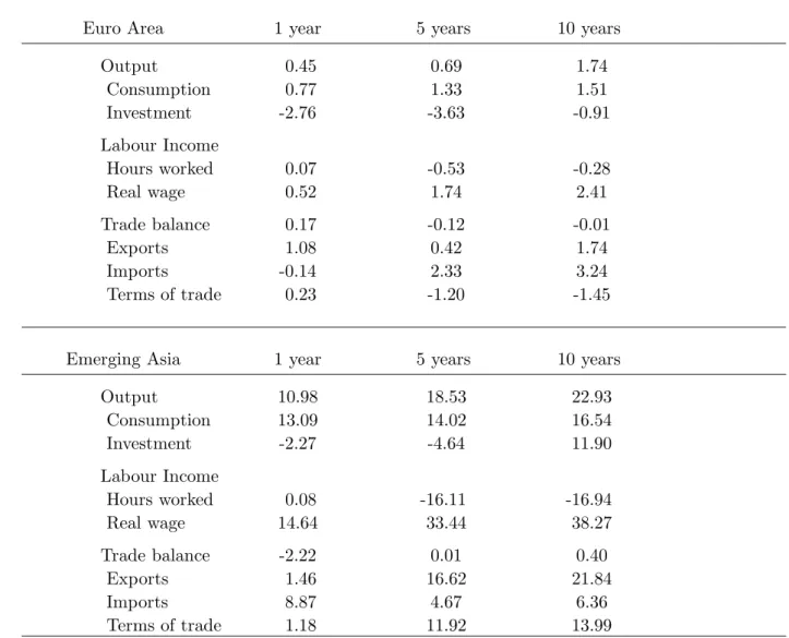
In Table 3, we report the transitional dynamics of scenario (I). In order to get a more realistic path for GDP and real consumption in emerging Asia, we also assume a persistent negative preference shock in the model, generated by an reduction in the time preference rate (discount factor), which triggers a subdued response of consumption and output on impact. Furthermore, we assume that the TFP spillover to the euro area is not taking place contemporaneously, but only 6 quarters after the TFP shock in emerging Asia. Note, however, that the TFP spillover is assumed to be anticipated. The results provide some interesting insights into the transitional dynamics of the globalisation shock.

First, while the response of output and consumption is positive, the reaction of in-vestment is negative for the first 10 years. The latter is driven by the expected rise of productivity in the long-run (determined by the assumed concave path of TFP following the shock) and the corresponding postponement of real investment. Note also that the concave path of level TFP also implies a gradual change in the terms of trade in emerging Asia.

In emerging Asia, the rise in permanent income generates an increase in consumption, which also triggers a demand for imported goods as they are necessary for the production of final consumption goods (level effect in emerging Asia). However, the impact of relative price changes in the rest of the world is subdued due to import adjustment costs, therefore the impact on real exports from emerging Asia is dampened (composition effect in the rest of world). Both factors lead to an initial deterioration of the trade balance.

In the euro area, the relative price of domestic goods falls, as the impact coming from emerging Asia is still limited, but price of imported goods from the US and the remaining countries remain relatively high. Although, import adjustment costs exclude a substantial immediate adjustment, aggregate imports do fall in the first year. Interestingly in both

cases the rise (deterioration) of the terms imply a negative wealth effect also indicated by the rise in hours worked. In the following years, as real quantities adjust, we observe a path for the macroeconomic variables, which are consistent with the long-run behaviour of the model.

6

Structural Reforms in the Euro Area and Globalisation

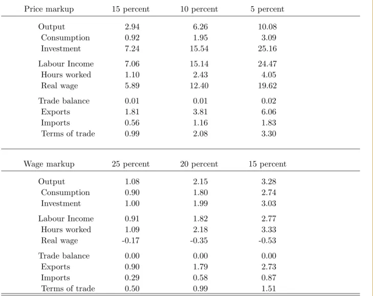
A widely discussed question in policy circles is how the euro area economy should react to the recent wave of globalisation? Are there any concrete policy measures or recommendations that we can derive from the model based analysis? One widely used argument is that goods and labour markets in the euro area should be made more flexible for being able to adjust faster to challenges and opportunities associated with globalisation. In what follows, we analyse the impact of structural reforms in goods and labour markets on the euro area economy conditional on a shock that we have above associated with the process of globalisation (column 1 in Table 2). In table 4, we present the results of this exercise. In particular, we simulate the model following the globalisation scenario for different degrees of monopolistic competition in goods and labour markets in the euro area. Note that all results are in deviation from the benchmark scenario, which has been conducted by assuming a price and wage markup of 20 and 30 percent respectively. The results indicate that structural reforms can amplify the positive effects of globalisation, as exemplified in the relative responses of output, consumption and investment. The results also give an indication that both scenarios would have significantly different impact on real wages in the euro area. While structural reforms in the goods market have a positive impact on real wages, labour market reforms driven by a reduction in the monopoly power on the household side will result in a reduction of real wages.

In analysing these simulations, it is worth recalling the reasons behind the differential impact of goods and labour market reforms on euro area GDP. Increased competition across firms lowers the price markup and these firm increase output since they are now constrained in their ability to exploit their market power. The increase in output affects capital more

rise in hours worked is demand driven as also indicated by the substantial rise in real wages, which also triggers a substantial increase in labour income. Note, however, that these results and therefore the quantitative impact on GDP are sensitive to the assumed labour supply elasticity in the model. By contrast, increased competition in labour markets reduce the ability of workers to exploit their market power, which increases hours worked, but leads to a less pronounces adjustment of capital and output, and even to a reduction of real wages. In addition, note that the change in consumption is closely allied to the change in labour effort as, in steady state, the disutility of work has to be equated with the benefits of consumption.

7

Conclusion

In this paper, we used the multi-country version of the NAWM to assess the impact of globalisation on euro area aggregates. We have provided a model-based definition of glob-alisation associated with an increase in potential output in emerging Asia and its potential impact on total factor productivity in the euro area, and a reduction in technological and institutional constraints that have previously forced domestic firms and consumers to pur-chase more goods of domestic origin. The results indicate that globalisation has a positive impact on output, consumption and investment in the long-run. Furthermore, the positive impact of globalisation through the improvement in the terms of trade, and the correspond-ing positive wealth effect allows households to reduce their labour market participation rate in the long-run, while at the same time experiencing an increase in real income through the rise in real wages. We argue, however, that a change in the relative competitiveness, represented by a change in home bias in our model, might lead to a deterioration of the terms or trade in the long-run triggering a negative wealth effect. While the latter will increase euro area output through a rise in labour supply, aggregate consumption will fall. Additionally, we have provided evidence that structural reforms in the goods and labour markets in the euro area could help amplifying the benefits associated with globalisation.

References

Bayoumi, T., D. Laxton and P. Pesenti, 2004, “Benefits and Spillovers of Greater Compe-tition in Europe: A Macroeconomic Assessment”, ECB Working Paper No. 341, Eu-ropean Central Bank, April.

Chen, N., J. Imbs and A. Scott, 2004, “Competition, Globalization and the Decline of In-flation”, CEPR discussion paper, 4695.

Christiano,L., M. Eichenbaum, and C. Evans, 2005, “Nominal Rigidities and the Dynamic Effects of a Shock to Monetary Policy”, Journal of Political Economy, University of Chicago Press, vol. 113(1), pages 1-45, February.

Coenen, G., P. McAdam and R. Straub, 2005, “Tax Reform and Labour-Market Perfor-mance in the Euro Area: A Simulation-Based Analysis Using the New Area-Wide Model”, forthcoming in theJournal of Economic Dynamics and Control.

Coenen, G. and R. Straub, 2005, “Does Government Spending Crowd in Private Consump-tion? Theory and Empirical Evidence for the Euro Area”, International Finance, 8, 435-470.

Denis, P., K. McMorrow and W. R¨oger, 2006, “Globalisation: Trends, Issues and Macro Implications for the EU”, European Commission Papers Nr. 254.

De Walque, G., Smets, F., Wouters, R., 2005, “An Estimated Two-country DSGE Model for the Euro Area and the US Economy”, European Central Bank, mimeo.

Erceg, C. J., L. Guerrieri and C. Gust, 2005, “SIGMA: A New Open Economy Model for Policy Analysis”, International Finance Discussion Papers No. 835, Board of Gover-nors of the Federal Reserve System, July.

Jacquinot, P. and R. Straub, 2007, “The multi-country version of the NAWM”, mimeo. Kamin, S.B., M. Marazzi, and J.W. Schindler, 2006, “The Impact of Chinese Exports on

Global Import Prices”,Review of International Economics, 14(2), 179-201.

Rogoff, K., 2003, “Globalization and global disinflation”, Proceedings, Federal Reserve Bank of Kansas City, pages 77-112.

Samuelson, P., 2004, “Where Ricardo and Mill Rebut and Confirm Arguments of Main-stream Economists Supporting Globalization”, Journal of Economic Perspectives, American Economic Association, vol. 18(3), pages 135-146, Summer.

Sbordone A.M., 2007, “Globalization and Inflation Dynamics: The Impact of Increased Competition”, NBER, working paper, 13556.

Appendix A

In this section, we define in detail the behaviour of firms in the model, which clarify the role of openness and channels of international transmissions as discussed in the main text. For more details, see Jacquinot and Straub (2007).

Firms

There are three types of firms, tradable intermediate and nontradable intermediate goods firms and final goods firms. In the nontradable intermediate goods market, there are a continuum of monopolistically competitive firms indexed by f ∈ Sn, each of which pro-duces a single nontradable differentiated intermediate good, H_f,t, while tradable goods firms indexed byf ∈Sn, produce a single tradable differentiated intermediate good, Hf,t.

In the final goods market, there are three types of firms, which combine domestically-produced tradable intermediate and nontradable intermediate goods with imported inter-mediate goods into three distinct non-tradable final goods, namely a private consumption good,QCt , a private investment good,QIt, and a public consumption good,QGt .

Final-Good Firms

In each country there is a continuum of symmetric firms producing three final goods, QC_t

(the final consumption good),QI_t, (the final investment good) andQG_t (public good) under perfect competition. For simplification we will drop the firm indices in what follows.

The representative firm producing the non-tradable final private consumption good,

QC_t , combines purchases of a bundle of domestically-produced non-tradable goods, HC_t , with purchases of a bundle of tradable goods,TtC ,

QC_t = ⎛ ⎝_(1−νC)μC1 _HC 1− 1 μC t +νC 1 μC_TtC 1− 1 μC ⎞ ⎠ μC μC−1 , (3) where the parameter μC > 1 denotes the intratemporal elasticity of substitution between

the distinct bundles of tradable and non-tradable goods. The weight of the inputs in the consumption basket are defined as (1−νC) and νC respectively. The bundle of tradable

T_tC = ⎛ ⎜ ⎝ϑ 1 μC_T C H_tC 1− 1 μC_T + (1−ϑC) 1 μC_{T (1−Γ} IMC(IM_tC/QC_t ))IM_tC 1− 1 μC_T ⎞ ⎟ ⎠ μC_T μC_T−1 (4)

where H_tC is a bundle of domestically produced tradable and IM_tC is bundle of imported tradable goods, (which is defined, as we will discuss later, as a bundle of imported goods from all remaining economies),μC_T stands for the intratemporal elasticity of substitution between the distinct bundles of tradable domestic and imported goods, andϑC determines the share

of domestic tradable goods compared to imported goods. Notice that the consumption-good firm incurs a cost, Γ_IMC(IM_tC/QC_t), when varying the use of the bundle of imported goods in producing the tradable consumption good.

The final good firm takes as given the prices of three inputs and minimizes its costs subject to the technological constraint defined above. The corresponding demand functions forHC_t, T_tC, IM_tC, H_tC are defined as follows:

HC_t = (1−νC) P_H,t PC,t _−μC QC_t , T_tC = νC P_T,tC PC,t _−μC QC_t , H_tC = νCϑC PH,t PC,t _−μC T _PC T,t PC,t _μC T−μC QC_t, IMtC = νC(1−ϑC) ⎛ ⎝ PIM,tC PC,tΓ†_IMC_,t ⎞ ⎠ −μC T P_T,tC PC,t _μC T−μT _QC t 1−Γ_IMC(IM_tC/QC_t), where P_H,t, PH,t, P_T,tC , P_IM,tC are the corresponding prices of inputs, while Γ†_IMC_,t = 1− Γ_IMC(IM_tC/QC_t )−Γ_IM C(IMtC/QCt )IMtC represents the first order derivative of the import

adjustment cost functions with respect to imports and P_T,tC is the price of the composite basket of domestic and foreign tradables (imports) defined as:

P_T,tC =ϑC(PH,t)1−μCT + (1−ϑC) (PIM,t)1−μCT

1

The formal characterization of the investment sectors is similar with self-explanatory changes in the notation. As in Coenen, McAdam and Straub (2007), we assume that the government sector is subject to complete home bias. In our model this implies that the final public good QGt is a composite of different varieties of nontradable goods only. Demand for domestic tradable and nontradable intermediate goods

In the next step, we will consider the composition of the baskets of intermediate tradable and nontradable goods. Intermediate goods come in different varieties (brands) and are produced under monopolistic conditions. Tradable and nontradable intermediate goods are defined over a continuum of mass s, standing for the size of the country. Each nontradable good is produced by a domestic firm indexed by f ∈ Sn , while each tradable good is produced by a firm indexed by f ∈ Sn.

In what follows, we will focus first on the production of the final domestically produced nontradable consumption goodHC_t , but the formal characterization holds also for the trad-able goods sector. Defining as HC_f,t the use of the intermediate goods produced by the domestic firm f , we have HC_t = 1 sn 1 θ_H Sn HC_f,t1− 1 θ_H df θ_H θ_H−1 , (6) whereθ_H are the intratemporal elasticities of substitution between the differentiated inter-mediate nontradable goods.

With nominal prices for differentiated intermediate goodsfbeing set in monopolistically competitive markets, the consumption-good firm takes pricesP_H,f,tas given and chooses the optimal use of each differentiated intermediate good f and by minimising the expenditure for the bundles of intermediate nontradable goods subject to the aggregation constraints defined above. This yields the following demand functions for the domestic intermediate goods f : HCf,t = _s1_n P_H,f,t P_{H,t −θ} H HCt, (7)

defined as: P_H,t = 1 sn Sn P_H,f,t1−θHdf 1 1−θ_H (8) Aggregating across firms and accounting for the public demand of nontradables (assumed to have the same composition as private demand), we get the following total demand function for nontradable goods:

HC_f,t+HI_f,t +HG_f,t= P_H,f,t P_{H,t, −θ} H HC_t +HI_t +HG_t (9) Following the same steps we can derive the domestic demand schedule for the tradable intermediate good: Hf,tC +Hf,tI +Hf,tG = PH,f,t PH,t _−θH HtC +HtI (10)

Imported Goods Sector

The representative domestic firm producing the final imported consumption good, IM_tC

combines purchases of a bundle of imported goods IMtC,nusing a CES technology:

IM_tC = n ν_IMC,n 1 μC_IM IM_tC,n1− 1 μC_IM μC_IM μC_IM−1 , (11) where 0 ≤ν_IMC,n ≤ 1,NνC,n = 1 and μCIM is the elasticity of import substitution across

countries. The higher μC_IM, the easier it is to substitute imports from one country with imports from the other. The parameter ν_IMC,n determines the composition of import baskets across countries. Note that the share of consumption goods imports of total consumption imports from a generic country does not need to be the same as the share of investment goods imports of total investment imports. Looking at the individual components of the final-imported consumption good aggregator, IMtC,n is in analogy to the domestically produced

sector, a CES index of all varieties of all tradable intermediate goods produced by firmsfn

in countryn. In particular: IMtC,n = _s1_n 1 θn_IM Sn IM_fC,nn_{,t 1−} 1 θn_IM dfn θn_IM θn_IM−1 , (12)

note that snis the share of a generic country. Furthermore, θn_IM is the elasticity of substi-tution between intermediate tradable goods in the generic country n.

Taking the prices of imported goods as given, the final imported-good firm chooses a combination of imported goods that minimizes _N PtnIMtn subject to aggregation

con-straint (??). This yields the following demand functions for IM_fC,nn_,t :

IM_fC,nn_,t = 1 sn ⎛ ⎝PIM,fC,n n,t P_IM,tC,n ⎞ ⎠ −θn IM IMtC,n, (13)

CorrespondinglyP_IM,tC,n can be defined as:

P_IM,tC,n = 1 sn Sn P_IM,fC,n n_{,t 1−θ}n IM dfn 1 1−θn_IM (14) The aggregate imported good price index can be defined as follows:

PIM,tC = N ν_IMC,n P_IM,tC,n _1−μH C 1 1−μC_IM (15) Similar conditions hold for the investment imported-good sector.

Intermediate Non-tradable Good Firms

Each intermediate-good firm f produces its differentiated output using an increasing-returns-to-scale Cobb-Douglas technology,

H_f,t= maxz_H,tK_f,tα N_f,t1−α−ψ_H,0, (16) utilising as inputs homogenous capital services,K_f,t, that are rented from the members of household I in fully competitive markets, and an index of differentiated labour services,

N_f,t, which combines household-specific varieties of labour supplied in monopolistically competitive markets. The variable zt represents (total-factor) productivity which is

as-sumed to be identical across firms and which evolves over time according to an exogenous serially correlated process, ln(z_H,t) = (1−ρ_z,H)z_H +ρ_z,H ln(z_H,t−1) +ε_H,z,t, where z_H

determines the steady-state level of productivity. The parameter ψ_H represents the fixed cost of production.10

10_{The fixed cost of production will be chosen to ensure zero profits in steady state in the tradable and}

non-tradable sectors respectively. This in turn guarantees that there is no incentive for other firms to enter the market in the long run.

Capital and Labour Inputs

Taking the rental cost of capital RK,t and the aggregate wage index Wt (to be derived

below) as given, the firm’s optimal demand for capital and labour services must solve the problem of minimising total input costRK,tK_f,t+(1+τtWf)WtN_f,tsubject to the technology

constraint defined above. Here, τtWf denotes the payroll tax rate levied on wage payments

(representing the firm’s contribution to social security).

Defining as MC_f,t the Lagrange multiplier associated with the technology constraint, the first-order conditions of the firm’s cost minimisation problem with respect to capital and labour inputs are given, respectively, by α(H_f,t+ψ_H)/K_f,tMC_f,t = RK,t and (1−

α) (H_f,t+ψ_H)/N_f,tMC_f,t = (1 + τ_tWf)Wt, with the payroll tax rate τtWf introducing a

wedge between the firm’s effective labour cost and the marginal revenue of labour.

The Lagrange multiplier MC_f,t measures the shadow price of varying the use of capital and labour services; that is, nominal marginal cost. We note that, since all firms f face the same input prices and since they all have access to the same production technology, nominal marginal costMC_f,t are identical across firms; that is,MC_f,t=MC_H,t with

MC_H,t= 1

z_H,tαα(1−α)1−α (RK,t)

α_{((1 +τ}Wf

t )Wt)1−α. (17) Intermediate Tradable Good Firms

Each intermediate-good firm f produces its differentiated output using an increasing-returns-to-scale Cobb-Douglas technology,

Yf,t= max

ztKf,tα Nf,t1−α−ψH,0

, (18) utilising as inputs homogenous capital services, Kf,t, that are rented from the members of

householdIin fully competitive markets, and an index of differentiated labour services,Nf,t,

which combines household-specific varieties of labour supplied in monopolistically compet-itive markets. The variable zt represents (total-factor) productivity which is assumed to

be identical across firms and which evolves over time according to an exogenous serially correlated process, ln(zH,t) = (1−ρH,z)z+ρH,z ln(zH,t−1) +εH,z,t, where zH determines

the steady-state level of productivity. The parameter ψH represents the fixed cost of

pro-duction.11

Capital and Labour Inputs

Taking the rental cost of capital RK,t and the aggregate wage index Wt (to be derived

below) as given, the firm’s optimal demand for capital and labour services must solve the problem of minimising total input costRK,tKf,t+(1+τtWf)WtNf,tsubject to the technology

constraint. Here, τ_tWf denotes the payroll tax rate levied on wage payments (representing the firm’s contribution to social security).

Defining as MCf,t the Lagrange multiplier associated with the technology constraint,

the first-order conditions of the firm’s cost minimisation problem with respect to capital and labour inputs are given, respectively, by α(Yf,t +ψH)/Kf,tMCf,t = RK,t and (1−

α) (Yf,t+ψH)/Nf,tMCf,t= (1 +τtWf)Wt, with the payroll tax rateτtWf introducing a wedge

between the firm’s effective labour cost and the marginal revenue of labour.

The Lagrange multiplier MCf,tmeasures the shadow price of varying the use of capital

and labour services; that is, nominal marginal cost. We note that, since all firms f face the same input prices and since they all have access to the same production technology, nominal marginal cost MCf,t are identical across firms; that is, MCf,t =MCH,t with

MCH,t= 1

zH,tαα(1−α)1−α (RK,t)

α_{((1 +τ}Wf

t )Wt)1−α. (19)

11_{The fixed cost of production will be chosen to ensure zero profits in steady state. This in turn guarantees}

Appendix B

A- Macroeconomic Aggregates

E A U S E M R W

Output Share in World Output 0.23 0.30 0.09 0.37

Consumption to GDP C/Y 0.59 0.63 0.54 0.62

Investment to GDP I/Y 0.22 0.20 0.30 0.23

Government Spending to GDP G/Y 0.18 0.16 0.16 0.16 Trade Balance to GDP T B/Y 0.01 0.03 -0.02 -0.02 Net foreign Assets to GDP Bf /Y -0.52 -1.12 1.00 0.97

B- Household

E A U S E M R W

Population size s 0.200 0.200 0.300 0.300

Subjective discount factor β 0.993 0.993 0.993 0.993 Inverse of the intertemporal elasticity

of substitution

σ 2.000 2.000 2.000 2.000

Habit persistence κ 0.600 0.600 0.600 0.600

Inverse of the Frish elasticity of labour supply

ζ 2.000 2.000 2.000 2.000

Depreciation rate δ 0.025 0.025 0.025 0.025

Size of household J ω 0.250 0.250 0.500 0.250 Households Calvo parameter ξI,ξJ 0.750 0.750 0.750 0.750

Wage indexation χI,χJ 0.750 0.750 0.750 0.750

C- Intermediate-good firms

E A U S E M R W

Share of capital income αH,αO 0.300 0.300 0.300 0.300

Share of fixed cost in production ψH 0.200 0.154 0.143 0.200

ψO

TFP parameter z 1.000 1.000 1.000 1.000

Price elasticity of labour demand η 4.300 7.300 7.300 6.000 Price elasticity of specific labour

de-mand

ηI,ηJ 4.300 7.300 7.300 6.000

Firms Calvo parameter ξH 0.900 0.900 0.900 0.900

ξO 0.900 0.900 0.900 0.900

ξX 0.300 0.300 0.300 0.300

Price indexation χH,χO 0.500 0.500 0.500 0.500

χX 0.500 0.500 0.500 0.500

Note: The subscriptI stands for unconstrained andJ for liquidity constrained households in our model. Correspondingly, H stands for tradable, X for the exports sector and O for nontradable sector in the model.

D- Final-goods firms

E A U S E M R W

Quasi-share of domestic nontradable νC 0.650 0.700 0.650 0.700

goods νI 0.300 0.350 0.300 0.350

Quasi-share of tradable goods νT C 0.301 0.617 0.324 0.417

νT I 0.873 0.689 0.220 0.467

Price elasticity of goods demand μC, μI 0.500 0.500 0.500 0.500

μC_IM,μI_IM 1.500 1.500 1.500 1.500

μT C,μT I 2.500 2.500 2.500 2.500

Price elasticity of intermediate goods demand

θ 6.000 6.000 6.000 6.000

Note: The subscript C stands for consumption goods sector, andI for investment goods sector. Corre-spondingly, the subscriptsT CandT Istand for tradable consumption and investment goods sector, while

IM denotes imported goods sector. The parameterμC_IM denote therefore the elasticity between different type of imported goods in the imported consumption good sector. The parameter μT C stand for the

elasticity of substitution between domestic and imported tradable goods.

E- Fiscal and monetary authorities

E A U S E M R W

Government debt-to-output ratio B∗_Y 2.400 2.400 2.400 2.400 Sensitivity of lump-sum taxes to BY Φ_{T B} 0.100 0.100 0.100 0.100

Inflation target π∗ 1.020 1.020 n.a. 1.020

Interest rate inertia Φ_RR 0.950 0.950 0 0.950

Inflation gap Φ_R,Π 2.000 2.000 0 2.000

Output gap Φ_R,GY 0.100 0.100 0 0.100

Response to US dollar FX Φ_R,S 0 0 + inf 0.100

F- Adjustment and transaction costs

E A U S E M R W

Transaction cost γv1 0.029 0.029 0.029 0.029 γv2 0.150 0.150 0.150 0.150 Capital utilisation cost γu2 0.007 0.007 0.007 0.007 Investment adjustment cost γI 3.000 3.000 3.000 3.000

Import adjustment cost γIMC,γIMI 5.000 5.000 5.000 5.000

G- Trade matrix (imports as a share of nominal GDP) to/from E A U S E M R W Consumption goods E A - 0.006 0.023 0.120 U S 0.011 - 0.014 0.049 E M 0.027 0.027 - 0.063 R W 0.051 0.044 0.011 -Investment goods E A - 0.006 0.004 0.014 U S 0.006 - 0.012 0.023 E M 0.017 0.037 - 0.098 R W 0.032 0.031 0.017

-H- Import Market Shares (as a percentage of total imports): Benchmark Calibration

Euro Area United States Emerging Asia Rest of the World

Consumption

Euro Area - 4.47 15.54 79.98

United States 14.92 - 19.77 65.30

Emerging Asia 23.10 22.90 - 54.00

Rest of the World 47.46 42.10 10.43

-Investment

Euro Area - 25.74 15.62 58.64

United States 14.46 - 29.24 56.30

Emerging Asia 11.09 24.52 - 64.39

Rest of the World 40.26 39.01 20.73

-Note: The columns indicate the country of origin, while the rows indicate the consumption and investment sector in a particular market.

Table 1: Long-run Impact of Structural Shocks

Productivity Labour Supply Home Bias

Shock Shock Shock

Euro area Output -0.19 -0.19 0.23 Consumption 0.78 0.78 -0.59 Investment 0.27 0.27 0.08 Labour Income Hours worked -0.27 -0.27 0.20 Real wage 0.99 0.99 -0.77 Trade balance 0.01 0.01 0.43 Exports 0.82 0.82 5.40 Imports 4.26 4.26 2.00 Terms of trade -2.77 -2.77 3.02 Emerging Asia Output 40.00 40.00 0.09 Consumption 36.31 36.31 0.20 Investment 29.53 29.53 0.33 Labour Income Hours worked -9.77 47.09 -0.06 Real wage 51.17 -7.27 0.32 Trade balance 0.31 0.31 0.10 Exports 31.97 31.97 0.42 Imports 8.98 8.98 1.03 Terms of trade 25.92 25.92 -0.92

Note: The individual productivity and labour supply shocks in emerging Asia are calibrated to generate a 40 percent increase in real GDP in emerging Asia. While the negative home bias shock in the euro area is calibrated to trigger a 2 percent increase in euro area imports in the long-run.

Appendix C