Identification of the Aquifer Parameters from
Pumping Test Data by using a Hybrid
Optimization Approach
M. Tamer Ayvaz
1*and Gurhan Gurarslan
11 Department of Civil Engineering, Pamukkale University, Denizli, Turkey
[email protected], [email protected]
Abstract
The main objective of this study is to propose a linked simulation-optimization approach to determine the parameters of the confined and leaky-confined aquifers from the results of the pumping tests. In the simulation part of the proposed approach, the drawdowns at the given monitoring points and times are calculated by considering Theis and Hantush approaches for confined and leaky-confined aquifers, respectively. This simulation part is then integrated with a hybrid optimization approach where global exploration feature of the harmony search (HS) and strong local search capability of the generalized reduced gradient (GRG) approach of the spreadsheet Solver add-in are mutually integrated. The performance of the proposed approach is evaluated by considering two pumping test data for the confined and leaky-confined aquifers. Identified results indicated that the hybrid HS-Solver optimization approach provides better results than those obtained by using both curve matching and stand-alone HS approaches.
1
Introduction
Groundwater management is an important part of the water resources planning and management. Mathematical simulation models are the essential tools for developing sustainable management plans for groundwater resources which require of knowing the spatial distributions of aquifer parameters over the field. These parameter distributions are usually obtained by interpolating the point observations which are mostly determined by performing pumping tests. Note that most of these tests are conducted by extracting the groundwater with a constant rate and recording the corresponding drawdowns in different monitoring locations and times. After obtaining the time-drawdown data from pumping test results, the parameters of the aquifer system are traditionally determined by means of a manual curve
* Corresponding author
Engineering
Volume 3, 2018, Pages 147–154
matching approaches. Although these approaches are simple to employ, some errors might be introduced since the accuracy of these approaches is mostly dependent to the modeller’s ability (Huang and Yeh, 2008). Therefore, use of the simulation-optimization models becomes popular tools to determine the aquifer parameters.
The current literature includes various solution approaches that integrate different simulation and optimization models for determining the aquifer parameters. These models mainly differ in terms of the considered optimization approaches. Both deterministic and heuristic optimization approaches are used employed to the solution of aquifer parameter estimation problems. Although deterministic approaches such as conjugate gradient, Gauss-Newton, and Marquardt algorithms are efficient to solve the problem in reasonable times, they usually prone to finding the local optimum solutions if a special initial solution is not provided (Samuel and Jha, 2003). The reason of this problem is associated with the non-convex solution space of the groundwater optimization problems (Willis and Yeh, 1987; Sun, 1994). Consequently, heuristic optimization approaches such as simulated annealing (SA) (Huang and Yeh, 2008), genetic algorithm (GA) (Samuel and Jha, 2003), and particle swarm optimization (PSO) (Sahin, 2018) algorithms are preferred to use in the solution of aquifer parameter estimation problems. Note that heuristic approaches are usually inspired from some events in natural phenomena and usually find the global or near global optimum solutions no matter where the solution starts (Ayvaz et al., 2009). However, stand-alone use of these approaches may require long computation times to precisely find the global optimum solutions (Michalewicz, 1992). Therefore, hybrid optimization approaches are employed for solving the optimization problems with a non-convex solution space. The main philosophy of the hybrid optimization approaches is to integrate the global exploration feature of the heuristic approaches and strong local search ability of the deterministic optimization approaches. In these algorithms, the global exploration process starts with multiple starting points and explores the search space, and then, deterministic approaches find the optimum solution by taking the results of global exploration as their initial values (Ayvaz et al., 2009). This kind of an integration makes the solution of the problem more robust than both heuristic and deterministic optimization approaches by themselves (Shannon, 1998).
The main objective of this study is to propose a hybrid solution approach for solving the aquifer parameter estimation problems by using the pumping test data. In the proposed approach, drawdown values at given distance and times are calculated by using the Theis and Hantush equations for confined and leaky-confined aquifers, respectively. These solutions are then integrated to an optimization model where hybrid HS-Solver optimization approach is used. HS-Solver is a recently proposed hybrid optimization approach which integrates the heuristic harmony search (HS) algorithm and a generalized reduced gradient (GRG) approach in the spreadsheet Solver add-in as the global and local optimizers, respectively. The performance of the proposed hybrid approach is evaluated by considering two pumping test data for the confined and leaky-confined aquifers. Identified results indicated that the proposed hybrid approach provides better results than those obtained by using both curve matching and stand-alone HS approaches.
2
Model Development
In this section, the main structure of the proposed hybrid approach is presented. For this purpose, first, the mathematical formulations of the Theis and Hantush models are given, and then, how to integrate them to the hybrid HS-Solver optimization approach is presented.
2.1
Theis Model
𝑠(𝑟, 𝑡) = 𝑄
4𝜋𝑇𝑊(𝑢) (1)
where 𝑠(𝑟, 𝑡) is the drawdown at a distance 𝑟 and at a time 𝑡, 𝑄 is the pumping rate which is constant during test, 𝑇 is the transmissivity of the aquifer, 𝑢 is a dimensionless parameter, and 𝑊(𝑢) is the well function of 𝑢, which is also known as the Theis function. Dimensionless parameter of 𝑢 and well function of 𝑊(𝑢) are given as follows:
𝑢 =𝑟2𝑆
4𝑇𝑡 (2)
𝑊(𝑢) = ∫𝑢∞𝑒−𝑦𝑦 𝑑𝑦 (3)
where 𝑆 is the storage coefficient of the aquifer, 𝑡 is the time since the beginning of pumping, and 𝑦 is the variable of integration. Note that the well function in Equation (3) can also be expressed with the following series (Kresic, 1997):
𝑊(𝑢) = 𝑙𝑛0.5615
𝑢 + ∑ (−1)
𝑛+1 𝑢𝑛 𝑛∙𝑛! ∞
𝑛=1 (4)
In the proposed approach, the value of 𝑊(𝑢) is calculated by means of Equation (4) by taking the upper limit of 𝑛 is 100.
2.2
Hantush Model
Unsteady groundwater flow toward a fully penetrating well in a leaky-confined aquifer without aquitard storage is given by the Hantush model which is expressed as follows (Hantush and Jacob, 1955):
𝑠(𝑟, 𝑡) = 𝑄
4𝜋𝑇𝑊(𝑢, 𝑟 𝐵⁄ ) (5)
where 𝐵 is the leakage factor, and 𝑊(𝑢, 𝑟 𝐵⁄ ) is the well function for the leaky confined aquifer whose value is the function of 𝑢 and 𝑟 𝐵⁄ . Definition of 𝑊(𝑢, 𝑟 𝐵⁄ ) and 𝐵 are given as follows:
𝑊(𝑢, 𝑟 𝐵⁄ ) = ∫ 𝑒
(−𝑦−(𝑟/𝐵)24𝑦 )
𝑦 ∞
𝑢 𝑑𝑦
(6)
𝐵 = √𝑇𝑏′
𝐾′ (7)
where 𝑏′ and 𝐾′ are the thickness and hydraulic conductivity of the confining bed (aquitard). Note that 𝑊(𝑢, 𝑟 𝐵⁄ ) values are tabulated for different 𝑢 and 𝑟 𝐵⁄ values by numerically integrating Equation (6) on MATLAB before executing the HS-Solver approach. In the optimization process, values of 𝑊(𝑢, 𝑟 𝐵⁄ ) are determined by conducting a bilinear interpolation between these tabulated values for the calculated 𝑢 and 𝑟 𝐵⁄ values.
2.3
Hybrid HS-Solver Optimization Approach
memory. Geem et al (2001) first adapted these musical rules to solve engineering optimization problems as: i) new decision variable values are selected randomly from the possible range, ii) new decision variable values are selected from harmony memory, iii) new decision variable values are further replaced with other ones which are close to their current values. Combinations of these rules in an optimization framework allow obtaining a global optimum solution in HS optimization algorithm.
Nowadays, electronic spreadsheets have become necessary tools to perform various engineering computations. Almost all the commercially available spreadsheet products such as Excel® include a built-in Solver add-in for solving unconstrained and constrained optimization problems by means of the GRG approach (Frontline Systems, 2018). Since Solver works on Excel®, all its computational features are accessible from the Visual Basic for Applications (VBA) platform. Therefore, HS and Solver processes have been hybridized on VBA platform by developing three separate VBA modules. The first module is for the stand alone HS and can be directly used to solve any optimization problem. The second module is developed for calling the Solver, which is created by using the macro recording feature of Excel®. The last module is used to integrate the HS and Solver modules to generate a hybrid optimization approach. Note that there are two options to integrate the HS and Solver processes in the last module. In the first option, the entire search space is explored by HS, then Solver gets the best result of HS as a starting point to precisely find the global optimum solution. In the second option, both HS and Solver run simultaneously such that all the solutions of HS are subjected to local search by Solver based on a small probability of 𝑃𝑐 (Ayvaz and Geem, 2018). In the proposed approach, the second
option is considered by setting the probability of 𝑃𝑐= 0.10 for all the solutions. The required solution
parameters of HS-Solver are the harmony memory size (𝐻𝑀𝑆), harmony memory considering rate (𝐻𝑀𝐶𝑅), pitch adjusting rate (𝑃𝐴𝑅), fret width (fw), and the probability of 𝑃𝑐. A detailed description
of these parameters and HS can be found in Geem et al. (2001) and Ayvaz et al. (2009).
2.4
Problem Formulation
The aquifer parameters can be identified by integrating HS-Solver approach with Theis and Hantush models for the confined and leaky-confined aquifers, respectively. In this integration, HS-Solver approach generates the associated aquifer parameters and these parameters are used in the Theis and Hantush models to estimate the drawdown of 𝑠(𝑟, 𝑡) in Equations (1) and (5), respectively. After this process, value of the objective function is calculated by means of the estimated and observed drawdowns at given distance and times. Note that the objective function used in this study is the sum of square errors (𝑆𝑆𝐸) which is given as follows:
𝑆𝑆𝐸(𝑟) = ∑𝑛𝑡 (𝑠(𝑟, 𝑡) − 𝑠̃(𝑟, 𝑡))2
𝑡=1 (8)
where 𝑆𝑆𝐸(𝑟) is the calculated 𝑆𝑆𝐸 value at a distance 𝑟, 𝑛𝑡 is the number of monitoring time steps,
and 𝑠̃(𝑟, 𝑡) is the observed drawdown at a distance 𝑟 and at a time 𝑡 which is obtained from the results of pumping test. After calculation objective function value, the parameter values of the aquifer system are adjusted by HS-Solver approach in order to minimize the calculated 𝑆𝑆𝐸(𝑟) value. Note that decision variables of the optimization model are 𝑇 and 𝑆 for the confined and 𝑇, 𝑆, and 𝐵 for the leaky-confined aquifers.
3
Numerical Applications
Furthermore, both problems have been solved 2 times for the same initial solutions in order to evaluate the model performance for HS and HS-Solver approaches. The HS-Solver solution parameters are taken as: 𝐻𝑀𝑆 = 10, 𝐻𝑀𝐶𝑅 = 0.95, 𝑃𝐴𝑅 = 0.50, 𝑃𝑐= 0.10, and 𝑓𝑤 = (𝑥𝑗𝑚𝑎𝑥− 𝑥𝑗𝑚𝑖𝑛)/300 where 𝑥𝑗𝑚𝑎𝑥
and 𝑥𝑗𝑚𝑖𝑛 are the maximum and minimum limits of the jth decision variable.
3.1
Example 1: Confined aquifer
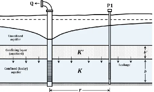
Figure 1 shows the confined aquifer system under consideration. A 24 hour pumping test is conducted to determine the 𝑇 and 𝑆. The pumping rate of 𝑄 is kept constant at 0.008 m3/s throughout
the test and the corresponding drawdowns at the piezometers of P1, P2, and P3 are recorded. By assuming 𝑟1= 5.5 m, 𝑟2= 40.5 m, and 𝑟3= 118 m in Figure 1, the problem is solved by using both
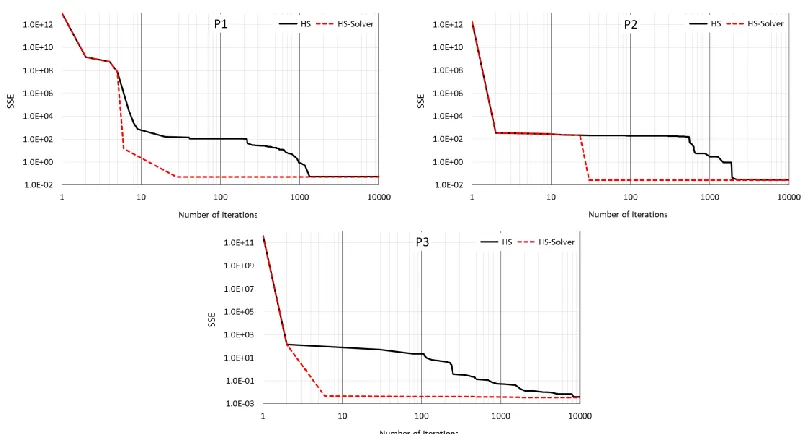
HS and HS-Solver based solution approaches. Figure 2 shows the convergence plots for both HS and HS-Solver approaches for each piezometer.
Figure 1: Cross-section of the confined aquifer under consideration
As can be seen from Figure 2, both HS and HS-Solver start the search process from the same initial solutions since the same random numbers seeds are used. Although both approaches have similar trend in the earlier stages of the optimization process, it is observed a significant improvement in the objective function value when the Solver is included to the HS solution. For these outcomes, Table 1 and 2 compare the model results with those obtained by using the manual curve matching approach. Table 1 states that although the identified 𝑇 and 𝑆 values well agree with the ones obtained from the curve matching approach for P2 and P3, there is a small difference in both 𝑇 and 𝑆 for P1. The reason of this difference is associated with the distance between pumping well and P1. Since P1 is the closest piezometer to the well location, its corresponding drawdowns are greater than those obtained in P2 and P3. Therefore, the recorded drawdown data of P1 are much less curved than for P2 and P3 and matching the theoretical Theis curve is more arbitrary as expected (Kresic, 1997). This outcome is also observed in Table 2 such that the calculated 𝑆𝑆𝐸 for P1 in the curve matching approach is approximately 10 times bigger than both HS and HS-Solver approaches. Note that Table 2 also includes a comparison of HS and Solver in terms of the number of required iterations. As can be seen, for each piezometer, HS-Solver finds better 𝑆𝑆𝐸 values by performing significantly fewer iterations than HS.
Solution approach P1 P2 P3
𝑇 (m2/day) 𝑆 (× 10−5) 𝑇 (m2/day) 𝑆 (× 10−5) 𝑇 (m2/day) 𝑆 (× 10−5)
Curve matching 119.23 8.70 130.46 4.70 129.60 5.20
HS 127.87 5.69 129.60 4.81 129.60 5.10
HS-Solver 128.74 5.46 128.74 4.92 131.33 4.96 Table 1: Comparison of the estimated 𝑇 and 𝑆 values for each piezometer
Solution approach 𝑆𝑆𝐸 Number of HS (Solver) Iterations
P1 P2 P3 P1 P2 P3
Curve matching 0.5497* 0.0306* 0.0056* N/A N/A N/A
HS 0.0529 0.0271 0.0039 1494 6378 9196
HS-Solver 0.0519 0.0264 0.0035 120 (83) 130 (45) 1858 (38) * This value is calculated by writing the results of Kresic (1997) into the Theis model.
Table 2: Comparison of the final 𝑆𝑆𝐸 values and number of required iterations (the values in the parentheses correspond to number of Solver iterations)
3.2
Example 2: Leaky-confined aquifer
Figure 3 shows the leaky-confined aquifer considered in this example. A pumping test is conducted at a fully penetrating well in a confined aquifer. The aquifer is overlain by an aquitard which is overlain by an unconfined aquifer. The test is conducted by considering a constant 𝑄 of 0.012 m3/s and the
Figure 3: Cross-section of the leaky-confined aquifer under consideration
Figure 4: Convergence plots of the HS and HS-Solver approaches
Solution approach 𝑇 (m2/day) 𝑆 (× 10−5) 𝐵 (m) 𝑆𝑆𝐸 Number of HS (Solver) Iterations
Curve matching 257.47 1.09 640.00 3.3678* N/A
HS 160.48 1.25 460.03 0.0754 9076
HS-Solver 159.93 1.26 457.90 0.0753 1053 (129) * This value is calculated by writing the results of Kresic (1997) into the Hantush model.
Table 3: Comparison of the estimated 𝑇, 𝑆, and 𝐵 values and final 𝑆𝑆𝐸 values and number of required iterations (the values in the parentheses correspond to number of Solver iterations)
4
Conclusions
In this study, the hybrid HS-Solver approach is first applied to the solution of aquifer parameter estimation problems by using the results of pumping tests. In the proposed approach, drawdown values at given distance and monitoring times are calculated by means of Theis and Hantush models for the confined and leaky-confined aquifers, respectively. These models are then used in conjunction with HS-Solver approach to determine the given aquifer parameters. Evaluation of the proposed approach is conducted by solving two pumping test examples. Identified results indicate that use of a simulation-optimization approach outperforms the inadequacy of the manual curve matching approach. Furthermore, use of a local search approach in a heuristic optimization approach significantly reduces the number of required iterations to find an optimum solution.
References
Ayvaz, M.T., Geem, Z.W. (2018). Optimum design of the booster chlorination systems by using hybrid HS-Solver optimization technique, PAJES (doi: 10.5505/pajes.2017.22587).
Ayvaz, M.T., Kayhan, A.H., Ceylan, H., Gurarslan, G. (2009). Hybridizing the harmony search algorithm with a spreadsheet 'Solver' for solving continuous engineering optimization problems,
Engineering Optimization, Vol. 41, pp. 1119-1144.
Frontline Systems (2018). Premium Solver’s web site. http://www.solver.com/premium-solver-platform#tab2
Geem, Z.W., Kim, J.H., Loganathan, G.V. (2001). A new heuristic optimization algorithm: Harmony Search, Simulation, Vol. 76, pp. 60-68.
Hantush, M.S., Jacob, C.E. (1955). Non-steady radial flow in an infinite leaky aquifer. Trans., Am. Geophys. Union, Vol. 36, pp. 95-100.
Huang, Y.C., Yeh, H.D., Lin, Y.C. (2008). A computer method based on simulated annealing to identify aquifer parameters using pumping-test data, Int. J. Numer. Anal. Meth. Geomech. Vol. 32, pp. 235–249.
Kresic, N. (1997). Quantitative solutions in hydrogeology and groundwater modelling, CRC Press, New York.
Michalewicz, Z. (1992). Genetic algorithm + data structure = evolution programs, Springer– Verlag, NewYork.
Sahin, A.U. (2018). A particle swarm optimization assessment for the determination of non-darcian flow parameters in a confined aquifer, Water Resources Management, Vol. 32, pp. 751-767.
Samuel, M.P., Jha, M.K. (2003). Estimation of aquifer parameters from pumping test data by genetic algorithm optimization technique, Journal of Irrigation and Drainage Engineering, Vol. 129.
Shannon, M.W. (1998). Evolutionary algorithms with local search for combinatorial optimization. Thesis (PhD), University of California, USA.
Sun, N.Z. (1994). Inverse problems in groundwater modeling, Kluwer Academic, Dordrecht, the Netherlands.
Theis, C.V. (1935). The relation between the lowering of the piezometric surface and the rate and duration of discharge of well using groundwater storage, Trans., Am. Geophysi. Union, Vol. 16, pp. 519–524.