Vol. 5, No. 4, 2013 Article ID IJIM-00263, 17 pages Research Article
Numerical solution of fuzzy differential equations under generalized
differentiability by fuzzy neural network
Maryam Mosleh ∗ †
————————————————————————————————–
Abstract
In this paper, We interpret a fuzzy differential equation by using the strongly generalized differen-tiability concept. Utilizing the Generalized characterization Theorem. Then a novel hybrid method based on learning algorithm of fuzzy neural network for the solution of differential equation with fuzzy initial value is presented. Here neural network is considered as a part of large field called neural computing or soft computing. The model finds the approximated solution of fuzzy differential equa-tion inside of its domain for the close enough neighborhood of the fuzzy initial point. We propose a learning algorithm from the cost function for adjusting of fuzzy weights.
Keywords: Fuzzy neural networks; Fuzzy differential equations; Feedforward neural network; Learning algorithm.
—————————————————————————————————–
1
Introduction
P
rquires detailed information of the system-oper design for engineering applications re-property distributions such as temperature, ve-locity, density, etc. in space and time domain [8, 9]. This information can be obtained by ei-ther experimental measurement or computational simulation. Although experimental measurement is reliable, it needs a lot of labor efforts and time. Therefore, the computational simulation has become a more and more popular method as a design tool since it needs only a fast com-puter with a large memory. Frequently, those engineering design problems deal with a set of∗Corresponding author. mosleh@iauf b.ac.ir
†Department of Mathematics, Firoozkooh Branch, Is-lamic Azad University, Firoozkooh, Iran.
differential equations (DEs), which have to nu-merically solved such as heat transfer, solid and fluid mechanics. Numerical methods of predictor-corrector, Runge-Kutta, finite difference, finite element, finite volume, boundary element, spec-tral and collocation provide a strategy by which we can attack many problems in applied math-ematics, where we simulate a real-word problem with a differential equation, subject to some ini-tial or boundary conditions. In the finite differ-ence and finite element methods we approximate the solution by using the numerical operators of the function’s derivatives and finding the solu-tion at specific preassigned grids [56]. The lin-earity is assumed for the purposes of evaluating the derivatives. Although such an approximation method is conceptually easy to understand, it has a number of shortcomings. Obviously, it is
cult to apply for systems with irregular geome-try or unusual boundary conditions. Predictor-corrector and Runge-Kutta methods are widely applied over preassigned grid points to solve or-dinary differential equations [35]. In the spectral and collocation approaches a truncated series of the specific orthogonal functions (basis functions) are used for finding the approximated solution of the DE. In the spectral and collocation techniques the role of trial functions as a basis function is important. The trial functions used in spectral methods are chosen from various classes of Ja-cobian polynomials [22], still the discretization meshes are preassigned. Neural network model is used to approximate the solutions of DEs for the entire domains. In 1990 the authors of [36] used parallel computers to solve a first order dif-ferential equation with Hopfield neural network models. Meade and Fernandez [39,40] solved lin-ear and nonlinlin-ear ordinary differential equations using feed forward neural networks architecture and B1-splines. Leephakpreeda [37] applied
neu-ral network model and linguistic model as uni-versal approximators for any nonlinear continu-ous functions. With this outstanding capability, the solution of DEs can be approximated by the appropriate neural network model and linguistic model within an arbitrary accuracy.
When a physical problem is transformed into a deterministic initial value problem
{ dy(x)
dx =f(x, y),
y(a) =A, (1.1)
We usually cannot be sure that this modelling is perfect. The initial value may not be known exactly and the functionf may contain unknown parameters. If the nature of errors is random, then instead of a deterministic problem (1.1) we get a random differential equation with random initial value and/ or random coefficients. But if the underlying structure is not probabilistic, e.g. because of subjective choice, then it may be appropriate to use fuzzy numbers instead of real random variables.
The topic of Fuzzy Differential Equations (FDEs) has been rapidly growing in recent years. The fuzzy initial value problem have been
stud-ied by several authors [1, 2, 6, 7,10, 50, 42, 43,
41, 13, 17, 51]. The concept of fuzzy derivative was first introduced by Chang and Zadeh [16], it was followed up by Dubois and Prade [19] who used the extension principle in their approach. Other methods have been discussed by Puri and Ralescu [49] and by Goetschel and Voxman [21]. Fuzzy differential equations were first formulated by Kaleva [32] and Seikkala [52] in time depen-dent form. Kaleva had formulated fuzzy differ-ential equations, in terms of Hukuhara derivative [32]. Buckley and Feuring [14] have given a very general formulation of a fuzzy first-order initial value problem. They first find the crisp solution, make it fuzzy and then check if it satisfies the FDE. In [48, 20], investigated the existence and uniqueness of solution for fuzzy random differen-tial equations with non-lipschitz coefficients and fuzzy differential equations with piecewise con-stant argument.
review relevant definition of the architecture of fuzzy neural networks. Section 3 gives details of problem formulation and the way to construct the fuzzy trial function and training of fuzzy neural network for finding the unknown adjustable co-efficients. Also, training of partially fuzzy neural network for finding the unknown adjustable coef-ficients.
2
Preliminaries
In this section the most basic notations used in fuzzy calculus are introduced. We start by defin-ing the fuzzy number.
Definition 2.1 A fuzzy number is a fuzzy setu:
R1−→I = [0,1]which satisfies i. u is upper semi-continuous.
ii. u(x) = 0 outside some interval [a, d]. iii. There are real numbers b, c:a≤b≤c≤d for which
1. u(x) is monotonic increasing on[a, b], 2. u(x) is monotonic decreasing on[c, d], 3. u(x) = 1, b,≤x≤c.
The set of all the fuzzy numbers (as given by Def-inition 2.1) is denoted by E1.
We briefly mention fuzzy number operations defined by the extension principle [57,58]. Since input vector of feedforward neural network is fuzzy in this paper, the following addition, mul-tiplication and nonlinear mapping of fuzzy num-bers are necessary for defining our fuzzy neural network:
µA+B(z) =max{µA(x)∧µB(y)|z=x+y}, (2.2)
µAB(z) =max{µA(x)∧µB(y)|z=xy}, (2.3) µf(N et)(z) =max{µN et(x)|z=f(x)}, (2.4)
where A, B, N et are fuzzy numbers, µ∗(.) de-notes the membership function of each fuzzy number, ∧ is the minimum operator and f(.) is a continuous activation function (like sigmoidal activation function) inside hidden neurons.
The above operations of fuzzy numbers are numerically performed on level sets (i.e.,α-cuts).
The h-level set of a fuzzy numberA is defined as
[A]h={x∈R|µA(x)≥h} f or 0< h≤1,
(2.5) and [A]0 =
∪
h∈(0,1][A]h. Since level sets of fuzzy
numbers become closed intervals, we denote [A]h
as
[A]h = [[A]Lh,[A]Uh], (2.6)
where [A]Lh and [A]Uh are the lower limit and the upper limit of the h-level set [A]h, respectively.
From interval arithmetic [5], the above operations of fuzzy numbers are written for h-level sets as follows:
[A]h+ [B]h= [[A]Lh + [B]Lh,[A]Uh + [B]Uh], (2.7)
[A]h.[B]h = [min{[A]Lh.[B]Lh,[A]Lh.[B]Uh,
[A]Uh.[B]Lh,[A]Uh.[B]Uh}, max{[A]Lh.[B]Lh,
[A]Lh.[B]Uh,[A]Uh.[B]Lh,[A]Uh.[B]Uh}], (2.8)
f([N et]h) =f([[N et]Lh,[N et]Uh]) =
[f([N et]Lh), f([N et]Uh)], (2.9) where f is increasing function.
Definition 2.2 [21] For arbitrary fuzzy numbers U, V, we use the distance
D(U, V) =sup0≤h≤1max{|[U]Lh −[V]|Lh,
|U]Uh −[V]Uh|}
and it is shown that (E, D) is a complete metric space.
Definition 2.3 Let U, V ∈ E. If there exists W ∈E, such that U =V +W, then W is called the H-difference of U, V and it is denotedU ⊖V.
In this paper the sign ⊖ always stands for the H-difference, and let us remark that U ⊖ V ̸= U + (−1)V. Usually we denote U+ (−1)V by U−V, whileU⊖V stands for the H-difference. In what follows, we fix X = (a, b), for a, b∈R.
limh−→0+
f(x0+h)⊖f(x0) h
and
limh−→0+
f(x0)⊖f(x0−h)
h ,
exist and are equal to F′(x0).
The above definition is a straightforward general-ization of the Hukuhara differentiability of a set-value function. From proposition 4.2.8 in [18], it follows that a Hukuhara differentiable function has increasing length of support. Note that this definition of a derivative is very restrictive [12]. The authors of [12] introduced a more general def-inition of a derivative for a fuzzy-number-valued function. In this paper we consider the following definition [15]:
Definition 2.5 Let f : X −→ E. Fix x0 ∈ X. We sayf is differentiable atx0, if there exists an element F′(x0)∈E such that
(1) for all h > 0 sufficiently close to 0, there exist f(x0+h)⊖F(x0), f(x0)⊖f(x0−h)and the limits (in the metric D)
limh−→0+
f(x0+h)⊖f(x0)
h =
limh−→0+
f(x0)⊖f(t0−h)
h =f
′(t 0), or
(2) for all h > 0 sufficiently close to 0, there exist f(x0+h)⊖f(x0), f(x0)⊖f(x0−h) and the limits (in the metric D)
limh−→0−
f(x0+h)⊖f(x0)
h =
limh−→0−
f(x0)⊖f(x0−h)
h =f
′(x 0).
Remark 2.1 [12] This definition agrees with the one introduced in [12]. Indeed, if f is differ-entiable in the senses (1) and (2) simultane-ously, then for h > 0 sufficiently small,, we have f(x0 +h) = f(x0) + U1, f(x0) = f(x0 − h) + U2, f(x0) = f(x0 +h) + V1 and f(x0) = f(x0 +h) +v2, with U1, U2, V1, V2 ∈ E. Thus, f(x0) = f(x0) + (U2 +V1), i.e.,U2+V1 = χ{0},
which implies two possibilities: U2 =V1 =χ{0} if f′(x0) =χ{0}; or U2 = χ{a} = −V1, with a∈ R, if f′(x0) ∈R.Therefore, if there exists f′(x0) in the first form (second form) with f′(x0) is not in R, then f′(x0) does not exist in the second form (first form, respectively).
Remark 2.2 In the previous definition, case (1) corresponds to the H-derivative introduced in [49], so this differentiability concept is a generalization of the H-derivative.
Remark 2.3 In [12], the authors consider four cases for derivatives. Here we only consider the two first cases od Definition 5 in [12]. In the other cases, the derivative is trivial because it is reduced to a crisp element (more precisely, f′ ∈ R; for details see Theorem 7 in [12]).
Definition 2.6 Let f : X −→ E. We say f is (1)-differentiable onXiff is differentiable in the sense (1) of Definition 7 and its derivative is de-noted D1f, and similarly for (2)-differentiability we have D2f.
The principal properties of defined derivatives are well known and can be found in [12,15]. In this paper, we make use of the following Theorem [15].
Theorem 2.1 Let f : X −→ E and put
[f(x)]h = [[f(x)]Lh,[f(x)]Uh]for each 0≤h≤1. (i) If f is (1)-differentiable then [f(x)]Lh
and [f(x)]Uh are differentiable functions and
[D1f(x)]h= [[f′(x)]Lh,[f′(x)]Uh].
(ii) If f is (2)-differentiable then [f(x)]Lh and
[f(x)]Uh are differentiable functions and we have
[D2f(x)]h= [[f′(x)]Uh,[f′(x)]Lh].
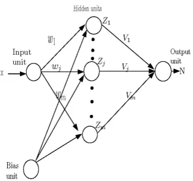
perceptron. Multi-layered perceptrons with more than three layers, use more hidden layers [25,33]. Multi-layered perceptrons correspond the input units to the output units by a specific nonlinear mapping [55]. From Kolmogorov existence the-orem we know that a three-layered perceptron with n(2n+ 1) nodes can compute any contin-uous function ofn variables [26]. Before
describ-Figure 1: Multiple layer feed-forward FNNM.
ing a fuzzy neural network architecture, we de-note real numbers and fuzzy numbers by lower-case letters (e.g., a, b, c, . . .) and uppercase letters (e.g., A, B, C, . . .), respectively.
Our fuzzy neural network is a three-layer feedforward neural network where connection weights, biases and targets are given as fuzzy numbers and inputs are given as real numbers. For convenience in this discussion, FNNM with an input layer, a single hidden layer, and an out-put layer in Fig. 1is represented as a basic struc-tural architecture. Here, the dimension of FNNM is denoted by the number of neurons in each layer, that isn×m×s, wherem, n andsare the num-ber of neurons in the input layer, the hidden layer and the output layer, respectively. The architec-ture of the model shows how FNNM transforms the n inputs (x1, . . . , xi, . . . , xn) into the s
out-puts (Y1, . . . , Yk, . . . , Ys) throughout the m
hid-den neurons (Z1, . . . , Zj, . . . , Zm), where the
cy-cles represent the neurons in each layer. Let Bj
be the bias for neuronZj, Ck be the bias for
neu-ron Yk, Wji be the weight connecting neuron xi
to neuron Zj, andWkj be the weight connecting
neuron Zj to neuron Yk.
2.1 Input-output relation of each unit
Let us consider a fuzzy three-layer feedforward neural network with n input units, m hidden units ands output units. Target vector, connec-tion weights and biases are fuzzy and input vector is real number. In order to derive a crisp learning rule, we restrict connection weights and biases by four types of (real numbers, symmetric triangu-lar fuzzy numbers, asymmetric triangutriangu-lar fuzzy numbers and asymmetric trapezoidal fuzzy num-bers) while we can use any type of fuzzy numbers for fuzzy targets. For example, an asymmetric triangular fuzzy connection weight is specified by its three parameters as Wkj = (wLkj, wCkj, wUkj).
When an n-dimensional input vector (x1, . . . , xi, . . . , xn) is presented to our fuzzy
neural network, its input-output relation can be written as follows, wheref :Rn−→Es:
Input units:
oi =xi, i= 1,2, . . . , n.
(2.10)
Hidden units:
Zj =f(N etj), j= 1,2, . . . , m,
(2.11)
N etj = n
∑
i=1
oi.Wji+Bj. (2.12)
Output units:
Yk=f(N etk), k= 1,2, . . . , s,
(2.13)
N etk= m
∑
j=1
The architecture of our fuzzy neural network is shown in Fig. 1 where connection weights, bi-ases, and targets are fuzzy and inputs are real numbers. The input-output relation in Eqs.(2.1 )-(2.14) is defined by the extension principle [57] as in Hayashi et al.[24] and Ishibuchi et al.[30].
2.2 Calculation of fuzzy output
The fuzzy output from each unit in Eqs.(2.1 )-(2.14) is numerically calculated for real inputs and level sets of fuzzy weights and fuzzy biases. The input-output relations of our fuzzy neural network can be written for theh-level sets: Input units:
oi =xi, i= 1,2, . . . , n.
(2.15)
Hidden units:
[Zj]h=f([N etj]h), j= 1,2, . . . , m,
(2.16)
[N etj]h= n
∑
i=1
oi.[Wji]h+ [Bj]h. (2.17)
Output unit:
[Yk]h =f([N etk]h), k= 1,2, . . . , s,
(2.18)
[N etk]h = m
∑
j=1
[Wkj]h.[Zj]h+ [Ck]h. (2.19)
From Eqs.(2.2)-(2.19), we can see that theh-level sets of the fuzzy outputsYk’s are calculated from
those of the fuzzy weights, fuzzy biases and crisp inputs. From Eqs.(2.7)-(2.9), the above relations are rewritten as follows when the inputs xi’s are
nonnegative, i.e., 0≤xi:
Input units:
oi =xi. (2.20)
Hidden units:
[Zj]h = [[Zj]Lh,[Zj]Uh] =
[f([N etj]Lh), f([N etj]Uh)], (2.21)
where f is increasing function.
[N etj]Lh = n
∑
i=1
oi.[Wji]hL+ [Bj]Lh, (2.22)
[N etj]Uh = n
∑
i=1
oi.[Wji]hU+ [Bj]Uh. (2.23)
Output units:
[Yk]h= [[Yk]Lh,[Yk]Uh] =
[f([N etk]Lh), f([N etk]Uh)], (2.24)
where f is increasing function.
[N etk]Lh =
∑
j∈a
[Wkj]Lh.[Zj]Lh+
∑
j∈b
[Wkj]Lh.[Zj]Uh + [Ck]Lh,
[N etk]Uh =
∑
j∈c
[Wkj]Uh.[Zj]Uh+
∑
j∈d
[Wkj]Uh.[Zj]Lh + [Ck]Uh, (2.25)
for [Zj]Uh ≥[Zj]Lh ≥0, where a ={j | [Wkj]Lh ≥
0}, b = {j | [Wkj]Lh < 0}, c = {j | [Wkj]Uh ≥
0},d={j |[Wkj]hU <0},a∪b={1, . . . , m} and c∪d={1, . . . , m}.
3
FDEs under generalized
dif-ferentiability
Let us consider the FDE
dy(x)
dx =f(x, y) (3.26)
initial value y(a) =A is given, we obtain a fuzzy Cauchy problem of first order:
{ dy(x)
dx =f(x, y), x∈[a, b],
y(a) =A, (3.27)
whereA is a fuzzy number inE withh-level sets
[A]h= [[A]Lh,[A]Uh], 0< h≤1.
Theorem 3.1 [15] Let f : X ×E −→ E be a continuous fuzzy function such that there exists k > 0 such that D(f(x, y), f(x, z)) ≤ kD(y, z), ∀x ∈ X, y, z ∈ E. Then problem (3.27) has two solution (one (1)-differentiable and the other one (2)-differentiable) on X.
Definition 3.1 Let y:X−→E be a fuzzy func-tion such that D1y or D2y exists. If y and D1y satisfy problem (3.27), we sayy is a (1)-solution of problem (3.27). Similarly, if y and D2y sat-isfy problem (3.27), we sayy is a (2)-solution of problem (3.27).
Let [y(x)]h = [[y(x)]Lh,[y(x)]Uh]. If y(x) is
(1)-differentiable then D1y(x) = [[y′(x)]Lh,[y′(x)]Uh],
and (3.27) translates into the following system of ODEs:
[y′(x)]Lh = [f(x, y)]hL, [y(a)]Lh = [A]Lh,
[y′(x)]Uh = [f(x, y)]hU, [y(a)]Uh = [A]Uh.
(3.28) Also, if y(x) is (2)-differentiable then D2y(x) =
[[y′(x)]Uh,[y′(x)]Lh], and (3.27) translates into the following system of ODEs:
[y′(x)]Lh = [f(x, y)]hU, [y(a)]Lh = [A]Lh,
[y′(x)]Uh = [f(x, y)]hL, [y(a)]Uh = [A]Uh,
(3.29) where [f(x, y)]h= [[f(x, y)]hL,[f(x, y)]Uh].The
au-thors of [15] state that if we ensure that the so-lution [[y(x)]Lh,[y(x)]Uh] of the system (3.28) are valid level sets of a fuzzy number valued func-tion and if [[y(x)]Lh,[y(x)]Uh] are valid level sets of a fuzzy valued function, then by the stacking
Theorem [32], it is possible to construct the (1)-solution of FDE (3.27). Also, for the (2)-solution, we can proceed in a similar way.
The Characterization Theorem [11] states that a FDE is equivalent to a system of ODEs under certain conditions.
Theorem 3.2 [46] Let us consider the FDE (3.27) where f :X×E −→E is such that
(i) [f(x, y)]h =
[[f(x,[y]Lh,[y]Uh)]Lh,[f(x,[y]Lh,[y]Uh)]Uh];
(ii) [f(x,[y]hL,[y]Uh)]Lh and [f(x,[y]Lh,[y]Uh)]Uh are equicontinuous;
(iii) there exists L >0 such that
|[f(x, y1, z1)]Lh −[f(x, y2, z2)]Lh|≤
Lmax{|y1−y2|,|z1−z2|}, ∀h∈[0,1];
|[f(x, y1, z1)]Uh −[f(x, y2, z2)]Uh|≤ Lmax{|y1−y2|,|z1−z2|}, ∀h∈[0,1]. Then, for (1)-differentiability, the FDE (3.27) and the system of ODEs (3.28) are equivalent and in (2)-differentiability, the FDE (3.27) and the system of ODEs (3.29) are equivalent.
Let us assume that a general approximation so-lution to Eq.(3.27) is in the form yT(x, P) for yT
as a dependent variable to x and P, where P
is an adjustable parameter involving weights and biases in the structure of the three-layered feed forward FNNM (see Fig. 2). The fuzzy trial so-lutionyT is an approximation solution toyfor the
optimized value of unknown weights and biases. Thus the problem of finding the approximated fuzzy solution for Eq. (3.27) over some colloca-tion points in [a, b] by a set of discrete equally spaced grid points
a=x1 < x2< . . . < xg =b,
is equivalent to calculate the functionalyT(x, P).
In order to obtain fuzzy approximate solution
yT(x, P), we solve unconstrained optimization
problem that is simpler to deal with, we define the fuzzy trial function to be in the following form:
Figure 2: Three layer fuzzy neural network with one input and one output.
where the first term in the right hand side does not involve with adjustable parameters and satis-fies the fuzzy initial condition. The second term in the right hand side is a feed forward three-layered fuzzy neural network consisting of an in-put x and the output N(x, P). The crisp trial function was used in [38]. In the next subsec-tion, this FNNM with some weights and biases is considered and we train in order to compute the approximate solution of problem (3.27).
Let us consider a three-layered FNNM (see Fig.
2) with one unit entryx, one hidden layer consist-ing ofmactivation functions and one unit output
N(x, P). In this paper, we use the sigmoidal ac-tivation functions(.) for the hidden units of our fuzzy neural network.
Here, the dimension of FNNM is 1×m×1. One drawback of fully fuzzy neural networks with fuzzy connection weights is long computa-tion time. Another drawback is that the learning algorithm is complicated. For reducing the com-plexity of the learning algorithm, we propose a partially fuzzy neural network (PFNN) architec-ture where connection weights to output unit are fuzzy numbers while connection weights and bi-ases to hidden units are real numbers [29, 42]. Since we had good simulation results even from partially fuzzy three-layer neural networks, we do not think that the extension of our learning algo-rithm to neural networks with more than three layer is an attractive research direction.
For every entry x the input neuron makes no changes in its input, so the input to the hidden neurons is
netj =x.wj+bj, j = 1, . . . , m, (3.31)
where wj is a weight parameter from input layer
to the jth unit in the hidden layer, bj is an jth
bias for the jth unit in the hidden layer. The output, in the hidden neurons is
zj =s(netj), j= 1, . . . , m, (3.32)
wheres(.) is the activation function which is nor-mally nonlinear function, the usual choices of the activation function [23] are the sigmoid transfer function, and the output neuron make no change its input, so the input to the output neuron is equal to output
N =V1z1+. . .+Vjzj +. . .+Vmzm, (3.33)
where Vj is a weight parameter from jth unit in
the hidden layer to the output layer. From Eqs. (2.20)-(2.25), we can be rewritten for h-level sets of the Eqs. (3.31)-(3.33). For reducing the complexity of the learning algorithm, input x
usually assumed as non-negative in fully fuzzy neural networks, i.e., 0≤x [28]:
Input unit:
o=x. (3.34) Hidden units:
zj =s(netj), j= 1, . . . , m, (3.35)
netj =o.wj+bj. (3.36)
Output unit:
[N]h= [[N]Lh,[N]Uh] =
[
m
∑
j=1
[Vj]Lh.zj, m
∑
j=1
[Vj]Uh.zj]. (3.37)
A P F N N4 (partially fuzzy neural network with
fuzzy differential equations? The training data are a = x1 < x2 < . . . < xg = b for input. We
propose a learning algorithm from the cost func-tion for adjusting weights.
Consider the following fuzzy initial value prob-lem for a first order differential equation (3.27), the related trial function will be in the form
yT(x, P) =A+ (x−a)N(x, P), (3.38)
this solution by intention satisfies the initial con-dition in (3.27). In [28], the learning of our fuzzy neural network is to minimize the dif-ference between the fuzzy target vector B = (B1, . . . , Bs) and the actual fuzzy output vector O = (O1, . . . , Os). The following cost function
was used in [28, 3] for measuring the difference betweenB and O:
e=∑
h eh =
∑ h h.{ s ∑ k=1
([Bk]Lh −[Ok]Lh)2/2
+
s
∑
k=1
([Bk]Uh −[Ok]Uh)2/2},
(3.39)
whereehis the cost function for theh-level sets of B andO. The squared errors between theh-level sets ofB andO are weighted by the value ofhin (3). In [29], it is shown by computer simulations that their paper, the fitting of fuzzy outputs to fuzzy targets is not good for the h-level sets with small values ofhwhen we use the cost function in (3). This is because the squared errors for theh -level sets are weighted byhin (3). Krishnamraju et al. [34] used the cost function without the weighting scheme:
e=∑
h eh=
∑ h { s ∑ k=1
([Bk]Lh −[Ok]Lh)2/2
+
s
∑
k=1
([Bk]Uh −[Ok]Uh)2/2}.
(3.40)
In the computer simulations included in this pa-per, we mainly use the cost function in (3) with-out the weighting scheme.
The error function that must be minimized for problem (3.28) is in the form
e1 = g
∑
i=1 e1i =
g
∑
i=1
∑
h
e1ih=
g
∑
i=1
∑
h
{eL1ih+eU1ih}, (3.41)
where
eL1ih= ([
dyT(xi,P)
dx ] L
h −[f(xi, yT(xi, P))]Lh)2
2 ,
eU1ih= ([
dyT(xi,P)
dx ] U
h −[f(xi, yT(xi, P))]Uh)2
2 .
Also, the error function that must be minimized for problem (3.29) is in the form
e2 = g
∑
i=1 e2i =
g
∑
i=1
∑
h
e2ih=
g
∑
i=1
∑
h
{eL2ih+eU2ih}, (3.42)
where
eL2ih= ([
dyT(xi,P)
dx ]Lh −[f(xi, yT(xi, P))]Uh)2
2 ,
eU2ih= ([
dyT(xi,P)
dx ]Uh −[f(xi, yT(xi, P))]Lh)2
2 .
and {xi}gi=1 are discrete points belonging to the
interval [a, b] and in the cost functions (3.41) and (3.42)eL1ih, eL2ihcan be viewed as the squared er-rors for the lower limits and eU1ih, eU2ih the upper limits of the h-level sets. It is easy to express the first derivative ofN(x, P) in terms of the deriva-tive of the sigmoid function, i.e.
∂[N]Lh
∂x = m
∑
j=1
[Vj]Lh. ∂zj ∂netj
m
∑
j=1
[Vj]Lh.zj.(1−zj).wj, (3.43)
∂[N]Uh
∂x = m
∑
j=1
[Vj]Uh. ∂zj ∂netj
.∂netj ∂x = m
∑
j=1
[Vj]Uh.zj.(1−zj).wj. (3.44)
Now differentiating from trial function yT(x, P)
in (3.42), we obtain
∂[yT(x, P)]Lh
∂x =
[N(x, P)]Lh + (x−a).∂[N(x, P)] L h
∂x ,
∂[yT(x, P)]Uh
∂x =
[N(x, P)]Uh + (x−a).∂[N(x, P)] U h
∂x ,
thus the expressions in (3.43) and (3.44) are ap-plicable here. A learning algorithm is derived in Appendix.
4
Example
In this section, we apply FNNM to an example. Consider the following FDE
Example 4.1 Consider the nuclear decay equa-tion
{ dy(x)
dx =−λy(x), y(0) =A,
wherey(x)is the number of radionuclides present in a given radioactive material, λ is the decay constant and A is the initial number of radionu-clides. In the model, uncertainty is introduced if we have uncertain information on the initial number A of radionuclides present in the mate-rial. Note that the phenomenon of nuclear dis-integration is considered a stochastic process, un-certainty being introduced by the lack of informa-tion on the radioactive material under study. In order to take into account the uncertainty we con-siderA to be a fuzzy number.
Letλ= 1, x∈[0,0.1]and[A]h= [h−1,1−h]. By using the Eq. (3.28) we get the exact solu-tion
[y1(x)]h = [(h−1)ex,(1−h)ex],
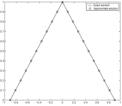
that is a (1)-differentiable solution of the problem (3.27). Using the Eq. (3.29) we get the exact solution
[y2(x)]h= [(h−1)e−x,(1−h)e−x],
is a (2)-differentiable solution of the problem (3.27).
In the interval [0,0.1] we consider a set of dis-crete equally spaced grid points 0 = x1 < 0.01 < ... < 0.1 and for Eq. (3.28) and Eq. (3.29) the approximate solutions are denoted by y1T(x, P) and y2T(x, P), respectively.
Here, the dimension of PFNN is1×5×1. The error function for the m = 5 sigmoid units in the hidden layer and for g = 11 equally spaced points inside the interval[0,0.1]is trained. In the computer simulation of this section, we use the following specifications of the learning algorithm.
(1) Number of hidden units: five units.
(2) Stopping condition: 100 iterations of the learning algorithm.
(3) Learning constant: η = 0.1. (4) Momentum constant: α= 0.2.
(5) Initial value of the weights and biases of PFNN are shown in table 1, that we supposeVi=
(v(1)i , vi(2), vi(3)) for i= 1, . . . ,5.
Figure 3: Analytical solution y1 and
ap-proximate solutiony1T.
Figure 4: Analytical solution y2 and
ap-proximate solutiony2T.
radioactive decay better. Now, if we consider the same differential equation under Hukuhara dif-ferentiability, then the (1)-solution (it exists and is unique by theorems in [54]) has an increas-ing length of its support, which leads us to the conclusion that there is a possibility that the ra-dioactivity of the system increases as time goes on and even a non-zero possibility that it is negative. Fortunately, the real situation is different, and the radioactivity of a material always decreases with time and it cannot be negative. So, the (2)-solution models the radioactive decay better.
heighti 1 2 3 4 5
v(1)i -0.5 -0.5 -0.5 -0.5 -0.5
v(2)i 0 0 0 0 0
v(3)i 0.5 0.5 0.5 0.5 0.5
wi 0 0 0 0 0
bi 0 0 0 0 0
Table 4.1. The initial values of weights
5
Conclusion
Solving fuzzy differential equations (FDEs) under generalized differentiability by using universal ap-proximators (UA), that is, FNNM is presented in this paper. The problem formulation of the pro-posed UAM is quite straightforward. To obtain the ”Best-approximated” solution of FDEs, the adjustable parameters of FNNM are systemati-cally adjusted by using the learning algorithm.
In this paper, we derived a learning algo-rithm of fuzzy weights of tree-layer feedforward fuzzy neural networks whose input-output rela-tions were defined by extension principle. The ef-fectiveness of the derived learning algorithm was demonstrated by computer simulation on numeri-cal example. Since we had good simulation result even from partially fuzzy three-layer neural net-works, we do not think that the extension of our learning algorithm to neural networks with more than three layers is an attractive research direc-tion. Good simulation result was obtained by this neural network in shorter computation times than fully fuzzy neural networks in our computer sim-ulations.
Appendix
Derivation of a learning algorithm in PFNN
Let us denote the fuzzy connection weight
Vj to the output unit by its parameter values
as Vj = (v(1)j , . . . , v(q)j , . . . , vj(r)). The amount of
modification of each parameter value for problem (3.28) is written as [27]
△vqj(t) =−η g
∑
i=1 ∂e1ih
∂vj(q) +α.△v (q)
j (t−1),
and the amount of modification of each parameter value for problem (3.29) is written as:
vj(q)(t+ 1) =v(q)j (t) +△vj(q)(t),
△vqj(t) =−η g
∑
i=1 ∂e2ih
∂vj(q) +α.△v (q)
j (t−1),
where t indexes the number of adjustments, η is a learning rate (positive real number) and α is a momentum term constant (positive real number). Thus our problem is to calculate the derivatives
∂e1ih
∂v(jq) and ∂e2ih
∂vj(q). Let us rewrite ∂e1ih
∂v(jq) and ∂e2ih
∂v(jq) as
follows:
∂e1ih
∂vj(q)
= ∂e1ih
∂[Vj]Lh .∂[Vj]
L h
∂v(q)j
+ ∂e1ih
∂[Vj]Uh .∂[Vj]
U h
∂v(q)j ,
∂e2ih
∂vj(q)
= ∂e2ih
∂[Vj]Lh .∂[Vj]
L h
∂v(q)j
+ ∂e2ih
∂[Vj]Uh .∂[Vj]
U h
∂v(q)j .
In this formulation, ∂[Vj]Lh
∂vj(q) and ∂[Vj]Uh
∂vj(q) are easily
calculated from the membership function of the fuzzy connection weightVj.
On the other hand, the derivatives ∂e1ih
∂[Vj]Lh,
∂e1ih
∂[Vj]Uh,
∂e2ih
∂[Vj]Lh and
∂e2ih
∂[Vj]Uh are independent of the
shape of the fuzzy connection weight. They can be calculated from the cost functionse1ihande2ih
using the input-output relation of our fuzzy neu-ral network for the h-level sets. When we use the cost function with the weighting scheme in (3.41) and (3.42), ∂e1ih
∂[Vj]Lh,
∂e1ih
∂[Vj]Uh,
∂e2ih
∂[Vj]Lh and
∂e2ih
∂[Vj]Uh
are calculated as follows: [Calculation of ∂e1ih
∂[Vj]Lh
]
∂e1ih ∂[Vj]Lh
=δL1.[∂[N(xi, P)]
L h ∂[Vj]Lh
+ (xi−a). ∂zj
∂x
−∂[f(x, yT(xi, P))]Lh ∂[yT(xi, P)]Lh
.∂[yT(xi, P))] L h ∂[Vj]Lh
],
where
δL1 = ([dyT(xi, P)
dx ] L
h −[f(xi, yT(xi, P))]Lh),
∂[yT(xi, P))]Lh ∂[Vj]Lh
] = (xi−a).zj,
∂N(xi, P)]Lh ∂[Vj]Lh
=zj.
[Calculation of ∂e1ih
∂[Vj]Uh]
∂e1ih ∂[Vj]Uh
=δ1U.[∂N(xi, P)]
U h ∂[Vj]Uh
+ (xi−a). ∂zj
∂x
−∂[f(x, yT(xi, P))]Uh ∂[yT(xi, P)]Uh
.∂[yT(xi, P))] U h ∂[Vj]Uh
],
where
δ1U = ([dyT(xi, P)
dx ] U
h −[f(xi, yT(xi, P))]Uh),
∂[yT(xi, P))]Uh ∂[Vj]Uh
] = (xi−a).zj,
∂N(xi, P)]Uh ∂[Vj]Uh
=zj.
[Calculation of ∂e2ih
∂[Vj]Lh]
∂e2ih ∂[Vj]Lh
=δ2L.[∂[N(xi, P)]
U h ∂[Vj]Lh
+ (xi−a). ∂zj
∂x
−∂[f(x, yT(xi, P))]Lh ∂[yT(xi, P)]Lh
.∂[yT(xi, P))] L h ∂[Vj]Lh
],
where
δ2L= ([dyT(xi, P)
dx ] U
h −[f(xi, yT(xi, P))]Lh),
∂[yT(xi, P))]Lh ∂[Vj]Lh
] = (xi−a).zj,
∂N(xi, P)]Lh ∂[Vj]Lh
=zj.
[Calculation of ∂e2ih
∂[Vj]Uh]
∂e2ih ∂[Vj]Uh
=δ2U.[∂N(xi, P)]
L h ∂[Vj]Uh
+ (xi−a). ∂zj
∂x
−∂[f(x, yT(xi, P))]Uh ∂[yT(xi, P)]Uh
.∂[yT(xi, P))] U h ∂[Vj]Uh
where
δ2U = ([dyT(xi, P)
dx ] L
h −[f(xi, yT(xi, P))]Uh),
∂[yT(xi, P))]Uh ∂[Vj]Uh
] = (xi−a).zj,
∂N(xi, P)]Uh ∂[Vj]Uh
=zj.
In our partially fuzzy neural network, the con-nection weights and biases to the hidden units are real numbers. The non-fuzzy connection weight
wj to the jth hidden unit is updated in the same
manner as the parameter values of the fuzzy con-nection weightVj as follows:
wj(t+ 1) =wj(t) +△wj(t),
△wj(t) =−η g
∑
i=1 ∂eih ∂wj
+α△wj(t−1).
The derivative ∂e1ih
∂wj and
∂e2ih
∂wj can be
calcu-lated from the cost functioneih using the
input-output relation of our PFNN for the h-level sets. When we use the cost function with the weighting scheme, ∂e1ih
∂wj and
∂e2ih
∂wj are calculated as follows:
∂e1ih ∂wj
=δ1L.[∂[N(xi, P)]
L h ∂wj
+ (xi−a).[Vj]Lh.zj
+(xi−a).xi.[Vj]Lh.zj(1−zj)wj
−(xi−a).[Vj]Lh.zj2−2(xi−a).xi.[Vj]Lh.zj2
(1−zj)wj−(
∂[f(xi, yT(xi, P))]Lh ∂[yT(xi, P))]Lh
.∂[yT(xi, P)] L h ∂
w˙j+∂[f(xi, yT(xi, P))]Lh ∂[y
T(x,P))]Uh.
∂[yT(xi, P)]Uh ∂wj
)] +δU1.[∂N(xi, P)]
U h ∂wj
+
(xi−a).[Vj]Uh.zj + (xi−a).xi.[Vj]Uh.zj
(1−zj)wj−(xi−a).[Vj]Uh.zj2−
2(xi−a).xi.[Vj]Uh.zj2(1−zj)wj−
(∂[f(xi, yT(xi, P))]
U h ∂[yT(xi, P))]Lh
.∂[yT(xi, P)] L h ∂
w˙j+
∂[f(xi, yT(xi, P))]Uh ∂[yT(xi, P))]Uh
.∂[yT(xi, P)] U h ∂wj
)],
and
∂e2ih ∂wj
=δU2.[∂[N(xi, P)]
U h ∂wj
+ (xi−a).[Vj]Uh.zj
+(xi−a).xi.[Vj]Uh.zj(1−zj)wj
-(x˙i-a).
[Vj]Uh.zj2−2(xi−a).xi.[Vj]Uh.zj2(1−zj)wj−
(∂[f(xi, yT(xi, P))]
L h ∂[yT(xi, P))]Lh
.∂[yT(xi, P)] L h ∂
w˙j+
∂[f(xi, yT(xi, P))]Lh ∂[yT(x, P))]Uh
.∂[yT(xi, P)] U h ∂wj
)]+
δ2U.[∂N(xi, P)]
L h ∂wj
+ (xi−a).[Vj]Lh.zj+ (xi−a).
xi.[Vj]Lh.zj(1−zj)wj−(xi−a).[Vj]Lh.z2j−
2(xi−a).xi.[Vj]Lh.z2j(1−zj)wj−
(∂[f(xi, yT(xi, P))]
U h ∂[yT(xi, P))]Lh
.∂[yT(xi, P)] L h ∂
w˙j
+∂[f(xi, yT(xi, P))]
U h ∂[yT(xi, P))]Uh
.∂[yT(xi, P)] U h ∂
where
∂[N(xi, P)]Lh ∂wj
= ∂[N(xi, P)]
L h ∂zj
. ∂zj ∂netj
.
∂netj ∂wj
= [Vj]Lh.zj.(1−zj).xi,
∂[N(xi, P)]Uh ∂wj
= ∂[N(xi, P)]
U h ∂zj
. ∂zj ∂netj
.
∂netj ∂wj
= [Vj]Uh.zj.(1−zj).xi,
∂[yT(xi, P))]Lh ∂wj
= (xi−a).
∂[N(xi, P)]Lh ∂wj
,
∂[yT(xi, P))]Uh ∂wj
= (xi−a).
∂[N(xi, P)]Uh ∂wj
.
The non-fuzzy biases to the hidden units are updated in the same manner as the non-fuzzy connection weights to the hidden units.
References
[1] S. Abbasbandy, J. J. Nieto, M. Alavi, Tuning of reachable set in one dimensional fuzzy dif-ferential inclusions, Chaos, Solitons & Frac-tals 26 (2005) 1337-1341.
[2] S. Abbasbandy, T. Allaviranloo, O. Lopez-Pouso, J. J. Nieto, Numerical methods for fuzzy differential inclusions, Computers & mathematics with applications 48 (2004) 1633-1641.
[3] S. Abbasbandy, M. Otadi,Numerical solution of fuzzy polynomials by fuzzy neural network, Appl. Math. Comput. 181 (2006) 1084-1089.
[4] S. Abbasbandy, M. Otadi, M. Mosleh, Numer-ical solution of a system of fuzzy polynomials by fuzzy neural network, Information Sciences 178 (2008) 1948-1960.
[5] G. Alefeld, J. Herzberger, Introduction to In-terval Computations, Academic Press, New York, (1983).
[6] T. Allahviranloo, E. Ahmady, N. Ahmady,
Nth-order fuzzy linear differential eqations, Information Sciences 178 (2008) 1309-1324.
[7] T. Allahviranloo, N. Ahmady, E. Ahmady,
Numerical solution of fuzzy differential eqa-tions by predictor-corrector method, Informa-tion Sciences 177 (2007) 1633-1647.
[8] H. Md. Azamathulla, A. Ab. Ghani, N. A. Zakaria,ANFIS based approach for predicting maximum scour location of spillway, Water Management, ICE London 162 (6) 399-407.
[9] H. Md. Azamathulla, C. C. Kiat, A. Ab. Ghani, Z. A. Hasan, N. A. Zakaria, An ANFIS-based approach for predicting the bed load for moderately-sized rivers, Journal of Hydro-Environment Research, Elsevier & KWRA 3 (2009) 35-44.
[10] M. Barkhordari Ahmadi, N. A. Kiani, Dif-ferential transformation method for solving fuzzy differential inclusions by fuzzy par-titions, International Journal of Industrial Mathematics 5 (2013) 237-249.
[11] B. Bede, Note on ”Numerical solutions of fuzzy differential equations by predictor cor-rector method”, Information Sciences 178 (2008) 1917-1922.
[12] B. Bede, S. G. Gal, Generalizations of the differentiability of fuzzy number value func-tions with applicafunc-tions to fuzzy differential equations, Fuzzy Sets and Systems 151 (2005) 581-599.
[13] B. Bede, I. J. Rudas, A. L. Bencsik, First order linear fuzzy differential eqations under generalized differentiability, Information Sci-ences 177 (2007) 1648-1662.
[15] Y. Chalco-Cano, H. Roman-Flores, On new solutions of fuzzy differential equations, Chaos Solitons & Fractals 38 (2008) 112-119.
[16] S. L. Chang, L. A. Zadeh, On fuzzy map-ping and control, IEEE Trans. Systems Man Cybemet 2 (1972) 30-34.
[17] M. Chen, C. Wu, X. Xue, G. Liu, On fuzzy boundary value problems, Information Sciences 178 (2008) 1877-1892.
[18] P. Diamond, P. Kloeden, Metric spaces of fuzzy sets, World scientific, Singapore, (1994).
[19] D. Dubois, H. Prade, Towards fuzzy differ-ential calculus: Part3, differentiation, Fuzzy Sets and Systems 8 (1982) 225-233.
[20] W. Fei, Existence and uniqueness of solu-tion for fuzzy random differential equasolu-tions with non-lipschitz coefficients, Information Sciences 177 (2007) 4329-4337.
[21] R. Goetschel, W. Voxman,Elementary fuzzy calculus, Fuzzy Sets and Systems 18 (1986) 31-43.
[22] D. Gottlieb, S.A. Orszag, Numerical anal-ysis of spectral methods: theory and applica-tions, CBMS-NSF Regional Conference Series in Applied Mathematics 26, SIAM, Philadel-phia, (1977).
[23] M. T. Hagan, H. B. Demuth, M. Beale, Neu-ral Network Design, PWS publishing com-pany, Massachusetts, (1996).
[24] Y. Hayashi, J. J. Buckley, E. Czogala,Fuzzy neural network with fuzzy signals and weights, Internat. J. Intelligent Systems 8 (1993) 527-537.
[25] S. Haykin, Neural Networks:A Comprehen-sive Foundation, Prentice Hall, New Jersey, (1999).
[26] K. Hornick, M. Stinchcombe, H. White, Mul-tilayer feedforward networks are universal ap-proximators, Neural Networks 2 (1989) 359-366.
[27] H. Ishibuchi, K. Kwon, H. Tanaka, A learn-ing algorithm of fuzzy neural networks with triangular fuzzy weights, Fuzzy Sets and Sys-tems 71 (1995) 277-293.
[28] H. Ishibuchi, K. Morioka, I. B. Turksen,
Learning by fuzzified neural networks, Int. J. Approximate Reasoning 13 (1995) 327-358.
[29] H. Ishibuchi, M. Nii, Numerical analysis of the learning of fuzzified neural networks from fuzzy if-then rules, Fuzzy Sets and Systems 120 (2001) 281-307.
[30] H. Ishibuchi, H. Okada, H. Tanaka, Fuzzy neural networks with fuzzy weights and fuzzy biases, Proc. ICNN 93 (1993) 1650-1655.
[31] H. Ishibuchi, H. Tanaka, H. Okada, Fuzzy neural networks with fuzzy weights and fuzzy biases, Proceedings of 1993 IEEE Interna-tional Conferences on Neural Networks, 1993, pp. 1650-1655.
[32] O. Kaleva, Fuzzy differential equations, Fuzzy Sets and Systems 24 (1987) 301-317.
[33] T. Khanna, Foundations of Neural Net-works, Addison-Wesly, Reading, MA, (1990).
[34] P. V. Krishnamraju, J. J. Buckley, K. D. Relly, Y. Hayashi, Genetic learning algo-rithms for fuzzy neural nets, Proceedings of 1994 IEEE International Conference on Fuzzy Systems, 1994, pp. 1969-1974.
[35] J. D. Lamber, Computational Methods in Ordinary Differential Equations, John Wiley & Sons, New York, (1983).
[36] H. Lee, I. S. Kang, Neural algorithms for solving differential equations, Journal of Com-putational Physics 91 (1990) 110-131.
[37] T. Leephakpreeda, Novel determination of differential-equation solutions: universal ap-proximation method, Computational and Ap-plied Mathematics 146 (2002) 443-457.
using a hybrid neural network-Optimization method, Appl. Math. Comput. 183 (2006) 260-271.
[39] A. J. Meade Jr, A. A. Fernandez, The nu-merical solution of linear ordinary differen-tial equations by feedforward neural networks, Mathematical and Computer Modelling 19 (1994) 1-25.
[40] A. J. Meade Jr, A. A. Fernandez, Solution of nonlinear ordinary differential equations by feedforward neural networks, Mathemati-cal and Computer Modelling 20 (1994) 19-44.
[41] M. T. Mizukoshi, L. C. Barros, Y. Chalco-Cano, H. Romn-Flores, R. C. Bassanezi,
Fuzzy differential equations and the extention principle, Information Sciences 177 (2007) 3627-3635.
[42] M. Mosleh, M. Otadi, Simulation and eval-uation of fuzzy differential eqeval-uations by fuzzy neural network, Applied Soft Computing 12 (2012) 2817-2827.
[43] M. Mosleh, M. Otadi, Minimal solution of fuzzy linear system of differential equa-tions, Neural Computing and Applications 21 (2012) 329-336.
[44] M. Mosleh, M. Otadi, S. Abbasbandy, Eval-uation of fuzzy regression models by fuzzy neu-ral network, Journal of Computational and Applied Mathematics 234 (2010) 825-834.
[45] M. Mosleh, M. Otadi, S. Abbasbandy, Evalu-ation of fuzzy polynomial regression model by fuzzy neural network, Applied mathematical modelling 35 (2011) 5400-5412.
[46] J. J. Nieto, A. Khastan, K. Ivaz, Numerical solution of fuzzy differential equation under generalized differentiability, Nonlinear Anali-sis: Hybrid Systems 3 (2009) 700-707.
[47] M. Otadi, M. Mosleh, Simulation and eval-uation of dual fully fuzzy linear systems by fuzzy neural network, Applied mathematical modelling 35 (2011) 5026-5039.
[48] G. Papaschinopoulos, G. Stefanidou, P. Efraimidis, Existence, uniquencess and asymptotic behavior of the solutions of a fuzzy differential equation with piecewise constant argument, Information Sciences 177 (2007) 3855-3870.
[49] M. L. Puri, D. A. Ralescu, Differentials of fuzzy functions, J. Math. Anal. Appl. 91 (1983) 552-558.
[50] R. Rodriguez-Lopez,Comparison results for fuzzy differential eqations, Information Sci-ences 178 (2008) 1756-1779.
[51] O. Sedaghatfar, P. Darabi, S. Moloudzadeh,
A method for solving first order fuzzy differen-tial equation, International Journal of Indus-trial Mathematics 5 (2013) 251-257.
[52] S. Seikkala, On the fuzzy initial value prob-lem, Fuzzy Sets and Systems 24 (1987) 319-330.
[53] R. J. Schalkoff, Artificial Neural Networks, McGraw-Hill, New York, (1997).
[54] S. Song, C. Wu, Existence and uniqueness of solutions to the Cauchy problem of fuzzy differential equations, Fuzzy Sets and Systems 110 (2000) 55-67.
[55] J. Stanley, Introduction to Neural Networks, third ed., Sierra Mardre, (1990).
[56] J. Store, R. Bulirsch, Introduction to Nu-merical Analysis, second ed., Springer-Verlag, New York, (1993).
[57] L. A. Zadeh, The concept of a liguistic vari-able and its application to approximate rea-soning, Information Sciences 8 (1975) 199-249.