Continuation power flow method for voltage stability analysis

(1)

Volume 3, Issue 6, 2016 Available online at www.ijiere.com

International Journal of Innovative and Emerging

Research in Engineering

e-ISSN: 2394 - 3343 p-ISSN: 2394 - 5494

Continuation Power Flow Method for Voltage Stability Analysis

Vineeta S.Chauhan

a

_{, Rashmi Sharma}

a

_{, Hinal Shah}

c

a_{Asst. Professor Dept. of Electrical & Electronics Engineering} c_{Asst. Professor Dept. of Electrical Engineering}

Indus University, Ahmedabad, India. [email protected]@yahoo.com

ABSTRACT:

Stability of a power system is defined as ability of power system to regain its original equilibrium state after being subjected to disturbance. Voltage stability refers to the ability of a power system to maintain steady voltages at all buses in the system after being subjected to a disturbance from a given initial operating condition. Transient stability is concerned with stability of system by considering large disturbances of small time duration. Voltage stability is a problem in power system which is lack of reactive power support when heavily loaded or the network transfer capability is reduced due to disturbances. The problem of voltage stability concerns the whole power system, although it usually has a large involvement in one critical area of the power system. In this paper Continuous power Flow Technique is used for the analysis.

Keywords: Voltage Stability, Transient stability, power system

I. INTRODUCTION

Present day power systems are being operated closer to their stability limits due to economic and environmental constraints. Maintaining a stable and secure operation of a power system is therefore a very momentous and challenging issue. Voltage stability is intimately related with other aspects of power system steady-state and dynamic performance. Voltage stability is influenced by voltage control, reactive power compensation and management, rotor angle or synchronous stability, protective relaying and control centre operations. Current day power systems are associated with problems like voltage level on the different buses beyond the limits considering the loading of that bus, and voltage collapse occurrences leading to major blackout etc. Such difficulties require studying voltage stability carefully therefore, voltage stability analysis is very important for making system more efficient and reliable. Voltage instability is a kind of problem in power systems which are greatly loaded, faulted or have a lack of reactive power. The nature of voltage stability can be analyzed by investigative the production, transmission and consumption of reactive power. The problem of voltage stability concerns the whole power system, although it usually has a large involvement in one critical area of the power system.This paper basically describes the voltage stability phenomena. Voltage stability and voltage instability are defined and. Factors affecting the voltage stability with their best features are discussed along with voltage stability analysis, which shows the importance of PV and QV curve and voltage collapse point for deciding voltage stability margin with different methodologies for finding voltage collapse point (Maximum loading point) with their most excellent features.[8]

(2)

Volume 3, Issue 6, 2016

II. REACTIVE POWER CAPABILITY OF SYNCHRONOUS GENERATOR

Synchronous generators are the primary devices for voltage and reactive power control in power systems. According to power system security the most important reactive power reserves are located there. In voltage stability studies active and reactive power capability of generators is needed to consider accurately achieving the best results. The active power limits are due to the design of the turbine and the boiler. Active power limits are constant. Reactive power limits are more complicated, which have a circular shape and are voltage dependent. Normally reactive power limits are described as constant limits in the load-flow programs. The voltage dependence of generator reactive power limits is, however, an important aspect in voltage stability studies. The limitation of reactive power has three different causes: stator current, over-excitation and under-excitation limits. When excitation current is limited to maximum value, the terminal voltage is the maximum excitation voltage less the voltage drop in the synchronous reactance. The power system has become weaker, because the constant voltage has moved more remote from loads.[4]

2 2

2

2 max

max 2

r G

d d

V E

V

Q

P

X

 





--- (1)

2 2 2

max max

s s G

Q



V I



P

--- (2)

The voltage dependent limit of excitation current can be calculated from Equation (1) . Where, PG is active power of generator,

Emax is the maximum of electromotive force,

Xd is synchronous reactance and V is terminal voltage. The reactive power limit corresponding stator current limit can be calculated

from Equation (2).

III. CONTINUATION POWER FLOW METHOD

The purpose of continuation load flow is to find a continuum of load flow solution for a given load/generation change scenario at different loading condition. It is capable of solving the whole PV-curve. The singularity of continuation load flow equation is not a difficulty. Therefore, the voltage collapse point can be solved. The computation of the maximum loading point (MLP) or voltage collapse point (Critical Point) is essential in power systems operation and control. The continuation power flow (CPF) method is very robust, widely known to draw PV-curves with removing singularity of Jacobian matrix, and can be also used for computing the voltage collapse point. Continuation Power Flow method is completely different from the Homology type of continuation used for the optimal power flow which gives the problem of Jacobian singularity. The continuation power flow analysis uses an iterative process involving prediction and corrector step as shown in above fig. 2 From known initial solution (A), a tangent predictor is shown is used to estimate the solution (B) for a specified pattern of load increases. The correct step then find the exact solution (C) using CPF analysis with the system load assumed to be fixed. The voltage in further increase in load is then predicted based on a new tangent predictor. If new estimated load (D) is now beyond the maximum load on the exact solution, a corrector step with loads fixed would not converge, then find exact solution (E). As the voltage stability limit is reached, to find the exact maximum load size of load increases has to be reduced gradually during the successive predictor steps.[8]

(3)

Figure 3. Flow chart for continuation power flow[8]

IV.RESULTSAND DISCUSSION

Figure 4. Single line diagram for IEEE-30 bus system Figure 5. Diagram of IEEE -30 bus systems simulatedwith PSAT

(4)

Volume 3, Issue 6, 2016 Analysis of IEEE-30 Bus System with PSAT in MATLAB

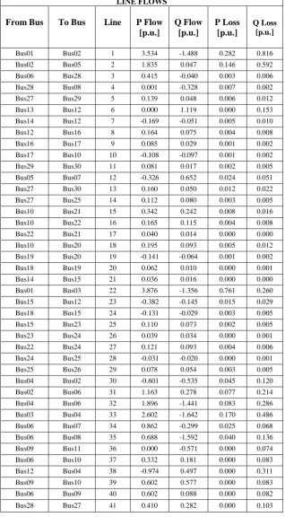
Line flow results & Power flow results

Table 1 LINE FLOWS From Bus To Bus Line P Flow [p.u.] Q Flow [p.u.] P Loss [p.u.] Q Loss [p.u.]

(5)

Volume 3, Issue 6, 2016 Table 2

POWER FLOW RESULTS

Bus No. V phase P gen Q gen P load Q load [p.u.] [rad] [p.u.] [p.u.] [p.u.] [p.u.]

Bus01 1.000 0.000 7.410 -2.845 0 0 Bus02 1.043 -0.224 0.855 3.556 0.464 0.272

Bus03 0.856 -0.146 0.000 0.000 0.513 0.026

Bus04 0.900 -0.303 0.000 0.000 0.163 0.034

Bus05 1.010 -0.574 0.000 1.603 2.015 0.406

Bus06 0.947 -0.416 0.000 0.000 0.000 0.000

Bus07 0.952 -0.503 0.000 0.000 0.488 0.233

Bus08 1.010 -0.466 0.000 2.701 0.642 0.642

Bus09 0.958 -0.551 0.000 0.000 0.000 0.000

Bus10 0.895 -0.628 0.000 0.000 0.124 0.042

Bus11 1.082 -0.551 0.000 0.645 0.000 0.000

Bus12 0.925 -0.586 0.000 0.000 0.240 0.160

Bus13 1.071 -0.586 0.000 1.119 0.000 0.000

Bus14 0.886 -0.631 0.000 0.000 0.133 0.034

Bus15 0.873 -0.636 0.000 0.000 0.175 0.053

Bus16 0.892 -0.617 0.000 0.000 0.075 0.038

Bus17 0.881 -0.636 0.000 0.000 0.192 0.124

Bus18 0.848 -0.670 0.000 0.000 0.068 0.019

Bus19 0.842 -0.681 0.000 0.000 0.203 0.073

Bus20 0.853 -0.670 0.000 0.000 0.047 0.015

Bus21 0.861 -0.651 0.000 0.000 0.374 0.240

Bus22 0.862 -0.650 0.000 0.000 0.000 0.000

Bus23 0.844 -0.656 0.000 0.000 0.068 0.034

Bus24 0.827 -0.665 0.000 0.000 0.186 0.140

Bus25 0.842 -0.656 0.000 0.000 0.000 0.000

Bus26 0.794 -0.680 0.000 0.000 0.075 0.049

Bus27 0.875 -0.636 0.000 0.000 0.000 0.000

Bus28 0.942 -0.444 0.000 0.000 0.000 0.000

Bus29 0.819 -0.702 0.000 0.000 0.051 0.019

(6)

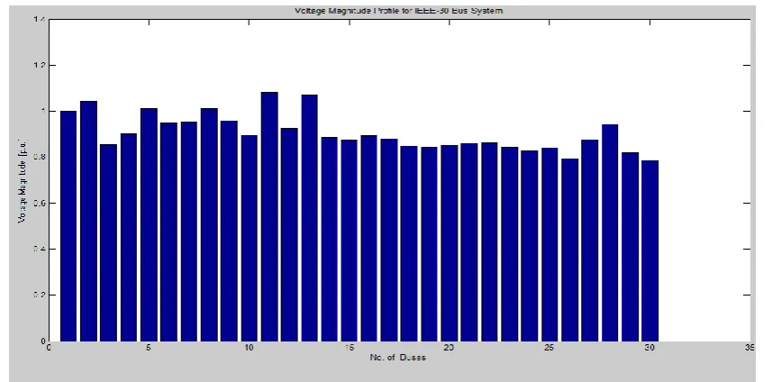
Figure 6.Voltage Magnitude Profile

P-V Curve for IEEE-30 Bus system

(7)

Analysis of Voltage Stability by Increasing Load

POWER FLOW RESULTS

Bus V phase P gen Q gen P load Q load

[p.u.] [rad] [p.u.] [p.u.] [p.u.] [p.u.]

Bus01 1.000 0.000 11.138 -2.687 0.000 0.000

Bus02 1.043 -0.332 0.837 5.467 0.591 0.346

Bus03 0.772 -0.189 0.000 0.000 0.653 0.033

Bus04 0.821 -0.438 0.000 0.000 0.207 0.044

Bus05 1.010 -0.818 0.000 2.479 2.564 0.517

Bus06 0.896 -0.611 0.000 0.000 0.000 0.000

Bus07 0.914 -0.729 0.000 0.000 0.621 0.297

Bus08 1.010 -0.690 0.000 4.480 0.816 0.816

Bus09 0.887 -0.822 0.000 0.000 0.000 0.000

Bus10 0.786 -0.952 0.000 0.000 0.158 0.054

Bus11 1.082 -0.822 0.000 1.013 0.000 0.000

Bus12 0.848 -0.895 0.000 0.000 0.305 0.204

Bus13 1.071 -0.895 0.000 1.709 0.000 0.000

Bus14 0.786 -0.967 0.000 0.000 0.169 0.044

Bus15 0.762 -0.973 0.000 0.000 0.223 0.068

Bus16 0.793 -0.938 0.000 0.000 0.095 0.049

Bus17 0.770 -0.966 0.000 0.000 0.245 0.158

Bus18 0.721 -1.029 0.000 0.000 0.087 0.024

Bus19 0.710 -1.045 0.000 0.000 0.259 0.093

Bus20 0.726 -1.026 0.000 0.000 0.060 0.019

Bus21 0.733 -0.992 0.000 0.000 0.476 0.305

Bus22 0.733 -0.990 0.000 0.000 0.000 0.000

Bus23 0.706 -1.009 0.000 0.000 0.087 0.044

Bus24 0.666 -1.026 0.000 0.000 0.237 0.180

Bus25 0.653 -1.025 0.000 0.000 0.000 0.000

Bus26 0.568 -1.080 0.000 0.000 0.095 0.063

Bus27 0.689 -0.995 0.000 0.000 0.000 0.000

Bus28 0.883 -0.650 0.000 0.000 0.000 0.000

Bus29 0.566 -1.149 0.000 0.000 0.065 0.024

(8)

LINE FLOW RESULTS

From Bus To Bus Line P Flow Q Flow P Loss Q Loss

[p.u.] [p.u.] [p.u.] [p.u.]

Bus01 Bus02 1 5.242 -1.572 0.574 1.692

Bus02 Bus05 2 2.532 0.178 0.280 1.153

Bus06 Bus28 3 0.542 0.066 0.006 0.017

Bus28 Bus08 4 0.000 -0.5662 0.025 0.061

Bus27 Bus29 5 0.202 0.109 0.025 0.047

Bus13 Bus12 6 0.000 1.707 0.000 0.356

Bus14 Bus12 7 -0.224 -0.077 0.011 0.023

Bus12 Bus16 8 0.210 0.136 0.008 0.017

Bus16 Bus17 9 0.107 0.069 0.001 0.005

Bus17 Bus10 10 -0.140 -0.093 0.002 0.004

Bus29 Bus30 11 0.112 0.038 0.011 0.020

Bus05 Bus07 12 -0.314 0.987 0.049 0.114

Bus27 Bus30 13 0.236 0.125 0.049 0.092

Bus27 Bus25 14 0.098 0.063 0.003 0.006

Bus10 Bus21 15 0.471 0.350 0.019 0.042

Bus10 Bus22 16 0.232 0.170 0.010 0.020

Bus22 Bus21 17 0.025 -0.003 0.000 0.000

Bus10 Bus20 18 0.257 0.121 0.012 0.027

Bus19 Bus20 19 -0.182 -0.069 0.003 0.005

Bus18 Bus19 20 0.077 0.025 0.001 0.002

Bus14 Bus15 21 0.055 0.033 0.001 0.001

Bus01 Bus03 22 5.682 -1.114 1.515 0.537

Bus15 Bus12 23 -0.503 -0.232 0.035 0.069

Bus18 Bus15 24 -0.165 -0.050 0.006 0.012

Bus15 Bus23 25 0.162 0.134 0.008 0.015

Bus23 Bus24 26 0.067 0.075 0.003 0.005

Bus22 Bus24 27 0.197 0.153 0.013 0.021

Bus24 Bus25 28 0.011 0.021 0.000 0.000

Bus25 Bus26 29 0.106 0.078 0.010 0.016

Bus04 Bus02 30 -0.789 -0.763 0.101 0.291

Bus02 Bus06 31 1.645 0.520 0.160 0.466

Bus04 Bus06 32 2.475 -1.938 0.174 0.601

Bus03 Bus04 33 3.514 -1.684 0.334 0.956

Bus06 Bus07 34 1.025 -0.455 0.042 0.121

Bus06 Bus08 35 0.959 -2.623 0.116 0.403

Bus09 Bus11 36 0.000 -0.831 0.000 0.182

Bus06 Bus10 37 0.438 0.308 0.000 0.186

Bus12 Bus04 38 -1.288 0.610 0.000 0.628

Bus09 Bus10 39 0.821 0.871 0.000 0.200

Bus06 Bus09 40 0.821 0.219 0.000 0.179

(9)

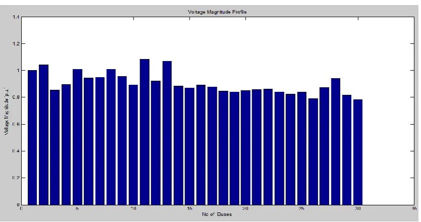
Voltage Magnitude Profile

Figure 7. Voltage Magnitude Profile

V .CONCLUSION

In this paper effect of continuation power flow in analyzing voltage stability is shown. It is very useful for evaluation of the critical point of the PV curve in static voltage stability assessment. PV- curves are constructed to calculate load ability margins and identify the weakest bus in the system. However, drawing the PV- curve is time consuming in large- scale power system. As a result, the open source power system analysis toolbox (PSAT) MATLAB software package is used for analysis. The results presented in this paper clearly show how CPF technique can be used to increase system load ability in power systems limits.

VI.REFERENCE

[1] G.K Morison, B. Gao, “voltage stability analysis using static and dynamic approaches”, IEEE transaction on power system, Vol. 8, No. 3, August 1993.

[2] S. Chakrabarti, Dept. of EE, IIT Kanpur “Notes on power system voltage stability.”

[3] B.Gao, G. K. Morison P. Kundur, “Voltage stability evaluation using Modal Analysis”, Transaction on power system, Vol. 7, No.4, November 1992.

[4] P. Kundur, John Paserba, Venkat Ajjarapu, “Definition and Classification of power system stability”, IEEE Transaction on power system, Vol. 19, No.2 May 2004.

[5] Thierry van cutsem, “Voltage instability: phenomena, countermeasure, and analysis methods.” Proceeding of the IEEE, VOL.88.NO.2, February 2000

[6] Farbod Larki, Mahmood Joorabian, “Voltage Stability Evaluation of The Khouzestan Power System in Iran Using CPF Method and Modal analysis”. IEEE Power and Energy Engineering Conference (APPEEC), 2010 Asia-Pacific

[7] ElFadilZakaria, amal Ramadan, Dalia Eltigani, “Method of Computing Maximum Load ability, Using Continuation Power Flow”, international conference on computing, electrical and electronic engineering (ICCEEE), 2013

[8] Prabha Kundur, “Power system stability and control” Tata McGraw-Hill Edition - 2011

[9] Abhijit Chakrabarti, Sunita Halder, “Power system analysis operation and control”, Third Edition, PHI publishers India [10] Ana Vitoria de, Almeida Macêdo, Benedito Antonio Luciano, Wellington Santos Mota “Influence of Voltage Stability in