Prediction of the pharmaceutical solubility in water and organic solvents via different soft computing models

(1)

*

Corresponding author: [email protected]

83 Research note

Prediction of the Pharmaceutical Solubility in Water and Organic

Solvents via Different Soft Computing Models

A. Yousefi, K. Movagharnejad *

Faculty of Chemical Engineering, Babol Noushiravani University of Technology, Babol, Iran

ARTICLE INFO ABSTRACT

Article history: Received: 2018-06-06 Accepted: 2018-11-11

Solubility data of solid in aqueous and different organic solvents are very important physicochemical properties considered in the design of the industrial processes and the theoretical studies. In this study, experimental solubility data of 666 pharmaceutical compounds in water and 712 pharmaceutical compounds in organic solvents were collected from different sources. Three different artificial neural networks, including multilayer perceptron, radial basis function, and support vector machine, were constructed to predict the solubility of these different pharmaceutical compounds in water and different solvents. Molecular weight, melting point, temperature, and the number of each functional group in the pharmaceutical compound and organic solvents were selected as the input variables of these three different neural network models. The neural network predictions were compared with the experimental data, and the SVR-PSO model with the Average Absolute Relative Deviation equal to 0.0166 for the solubility in water and 0.0707 for solubility in organic compounds was selected as the most accurate model.

Keywords:

Organic Compound, Solubility,

Artificial Neural Network, Group Contribution, Support Vector Machine

1.Introduction

Solubility is known as the maximum limit of solute dissolved in a solvent under specified conditions [1]. The IUPAC definition of solubility is an analytical composition of a saturated solution expressed as a proportion of a designated solute in a designated solvent [2]. The solubility is a strong function of intermolecular forces between the solute and solvent, describing the solvent-solute systems [3]. The solubility of a pharmaceutical in water and organic solvents is controlled by two types of interactions. The first interaction

(2)

84 Iranian Journal of Chemical Engineering, Vol. 16, No. 1 (Winter 2019)

different organic solvents is one of the most important physicochemical properties considered in the design of the industrial processes and the theoretical studies. Production and purification of pharmaceuticals [7], design and optimization of industrial crystallization processes [8], separation of organic products [9], and chemical reaction systems [10] are just some examples of the importance of this property. Therefore, accurate knowledge of the solubility of solute in a given solvent is very important for developing optimal processes. Experimental determination of the solubility is difficult and time-consuming; therefore, many researchers have attempted to predict solubility. Generally, these studies are divided into two main categories. The first category includes the thermodynamic models such as UNIFAC method [11], perturbed-chain statistical associating fluid theory (PC-SAFT) that predicts the solubility on the basis of the melting point and the enthalpy of fusion [12], and segment activity coefficient (COSMO-SAC) model that predicts the solubility on the basis of the available surface area of the solvent [13]. A new theoretical model has been recently published by Zhao et al. [14], which is based on an estimated equation of molar intermolecular potential energy for species in fluid mixtures [14]. However, this category of methods has been reported to have several drawbacks to estimate the pharmaceutical solubility in different solvents [15].

The second category is the mathematical/empirical/semi-empirical

correlations to predict the solubility. One of the first semi-empirical methods was

presented by Yalkowsky [16]. This

correlation was based on the entropy of fusion, melting point, and octanol-water

partition coefficient. Ruelle [17] predicted the solubility of pharmaceuticals using the mobile order theory considering the hydrophobic effect. Abraham and Le [18] used the linear solvation energy relationship (LSER) method based on the acidity and basicity of the solute, excess molar refractivity, polarizability of solute, and McGowan’s characteristic volume [18] to reach a new solubility correlation. Another method in this category may be the COSMO-RS, which is based on the quantum chemical calculations and Gibbs free energy of fusion [19]. Wang et al. [20] presented a method for solubility prediction using the atom types, the molecular polarizability, molecular weight, intermolecular hydrogen bonding, and hydrophobicity. The other methods are based on the quantitative structure–properties relationship (QSPR) such as group contribution [21] and atom contribution [22].

(3)

Iranian Journal of Chemical Engineering, Vol. 16, No. 1 (Winter 2019) 85

the results of several empirical methods. All of these researches have shown that the solubility is a strong function of temperature, melting point, and chemical functional groups of solute and solvent. The purpose of this study is to develop three types of neural networks: multilayer perceptron (MLP), radial basis function (RBF), and support vector machine (SVM) based on the group contribution method (GC) and particle swarm optimization algorithm (PSO) for exact and comprehensive predictions of pharmaceutical solubility in water and organic solvents.

2. Theory

Artificial neural networks are mathematical models that fall into the category of

computational intelligence tools. These

networks are able to process a large quantity of data and achieve a generalized result. ANN models are powerful tools for function approximation, classification, and prediction by adjusting appropriate parameters [27]. The aim of this research is to develop different MLP, RBF, and SVR models and analyze their performance. The particle swarm optimization algorithm is also used to optimize the performance of the neural networks.

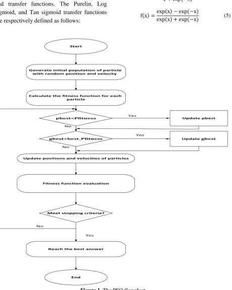
2.1. Particle swarm optimization algorithm

Particle swarm optimization algorithm is an

optimization technique, introduced by

Kennedy & Eberhart [28]. The main idea of this method is based on the collective motion of groups of animals such as birds and fishes to find food without any previous knowledge about its position.

In this algorithm, it is assumed that, in an n-dimensional search space, the total number of particles is m, particle is the optimization

variable shown by x=

(

x1,x2,2,xm

)

, and

each particle in the position of the space is

presented by xi =

(

xi,1,xi,2,2,xi,n,i

)

T, with the

velocity of the ith particle

(

)

T

n i i

i

i v v v

v = _,₁, _,₂,2, _, . The value of the local

best position of the ith particle is shown by

(

)

T

n i i

i

i p p p

p = ,1, ,2,2, , , and the global best

position of all particles is presented by

(

)

T

n g g

g

g p p p

p = _,₁, _,₂,2, _, . After finding the

local and global best positions, the velocity and the new location of each particle are updated with the following equations. These steps will continue several times until the desired answer is achieved.

vij(t + 1) = w vij(t) + r1c1�pij(t)−xij(t)�+ r2c2 (gj(t)−xij(t)) (1)

xij(t + 1) = xij(t) + vij(t + 1) (2)

where i= 1…, m; 𝑥𝑥_{𝑖𝑖𝑖𝑖}(𝑡𝑡) and 𝑣𝑣_{𝑖𝑖𝑖𝑖}(𝑡𝑡) denote the position and velocity of the ith particle in j-dimension and the tth iteration, respectively;

𝑤𝑤 denotes the inertia weight; 𝑐𝑐₁ and 𝑐𝑐₂ are acceleration coefficients; 𝑟𝑟₁ and 𝑟𝑟₂ are random numbers with a uniform distribution;

𝑝𝑝𝑖𝑖𝑖𝑖(𝑡𝑡) denotes the best position of the ith particle in j-dimension; 𝑔𝑔_𝑖𝑖(𝑡𝑡) denotes the

global best position [28]. The flowchart of this algorithm is shown in the Figure 1.

2.2. Multilayer perceptron network

(4)

neuron. MLP network is a multi-layer structure of neurons linked to each other with the weight connections matrix, bias vectors, and transfer functions. The Purelin, Log sigmoid, and Tan sigmoid transfer functions are respectively defined as follows:

f(x) = x (3)

f(x) =_{1 + exp (}1 ₋_x) (4)

f(x) =exp(x)−exp(−x)

exp(x) + exp(−x) (5)

Figure 1. The PSO flowchart.

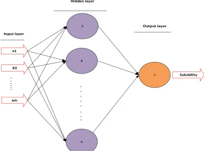
A typical MLP that is shown in Figure 2 consists of at least 3 layers. These layers include an input layer that receives the input

variables from the outside, one or more hidden layer(s) to estimate the output variables using the weight matrix, and an Start

Generate initial population of particle with random position and velocity

Calculate the fitness function for each particle

Update positions and velocities of particles

Fitness function evaluation

Meet stopping criteria?

Reach the best answer Pfitness <

pbest

Pfitness _

best < gbest

Update pbest

Update gbest

End

Yes No

Yes

No

Yes

(5)

output layer to present the output variable(s). The process of tuning the weights and biases using a training dataset that contains the experimental inputs and outputs is called the supervised Training Algorithm. There are two supervised methods for training the network

and determining the neural network

coefficients. The first category is called the classical algorithms such as back propagation algorithm as one of the most popular

algorithms, and the second category is called the intelligent algorithms such as particle swarm optimization algorithm for training MLP. All of these methods are used to obtain the optimized connection weights and biases [29, 30]. The number of hidden layers, the type of the transfer function, and the general structure of the neural network are obtained by the trial-and-error approach.

Figure 2. Schematic diagram of the three layer MLP.

2.3. Radial basis function neural network (RBF)

Radial basis function (RBF) networks are another type of feed-forward networks, which were introduced by D.S. Broomhead and David Lowe [30]. This type of network is based on the supervised learning methods and is a general approach to the quantization of information. MLP and RBF networks can be applied for the similar type of applications with the relatively same structure, yet

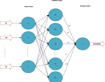
different internal computation methods. A schematic diagram of an RBF neural network consisting of three layers is shown in Figure 3: (a) an input layer that does not process the information and only distributes the input vectors to the hidden layer, (b) a hidden layer that converts 𝑛𝑛-dimensional input space to 𝑚𝑚 -dimensional feature space (𝑚𝑚 ≥ 𝑛𝑛) with nonlinear function mapping, and (c) an output layer.

1

2

n

1 Solubility

x1 Input layer

Hidden layer

Output layer

X2

. .

. . . . _{. .}

.

(6)

88 Iranian Journal of Chemical Engineering, Vol. 16, No. 1 (Winter 2019) Figure 3. Schematic diagram of RBF.

The output of the output layer can be determined by a linear combination of the kernel functions, which is defined as follows:

y = wT_ϕ_{(x) =}_�_w iϕi(x) m

i=1

+ b (6)

where 𝑤𝑤 is the weight vector, b is the bias,

𝜙𝜙(𝑥𝑥) is the kernel function defined as a function whose value depends only on the distance of 𝑥𝑥from 𝑥𝑥₀, and ||∗|| denotes the Euclidean norm as in the following:

ϕ(x) = f(r) = f(||x−x0||) (7)

There are many kernel functions such as the polynomial, Gaussian, and multiquadric functions. The Gaussian function is used in this study:

ϕi(x) = (−1₂�x−_σmi

i �

2

) (8)

By substitution of Eq (8) in Eq (6), the output

of the RBF neural network is computed according to Eq (9).

y =�wiexp (−1₂�x−_σmi

i �

2 ) n

i=0

(9)

where 𝑤𝑤_𝑖𝑖 is the weight connection from the hidden layer to the output layer, 𝑚𝑚_𝑖𝑖 is the center of each neuron in the radial basis function, and 𝜎𝜎_𝑖𝑖 is the spread parameter of the ith kernel [31]. The learning algorithm for determining these parameters consists of two sections. The first section consists of random sampling of input samples. The main parameters of kernel function center (𝑚𝑚_𝑖𝑖) of neurons in the hidden layer and the spread (𝜎𝜎𝑖𝑖) are determined in this section. The second section consists of training the weights that link the hidden layer to the output layer [32].

2.4. Support vector regression

1

2

n

Ø0

Ø1

Øm Ø2

Øi

1 Solubility

Input layer

Hidden layer

Output layer

w0

w2 w1

wi

wm x1

X2

. . . . .. . . . . . . . .

. . .

.

(7)

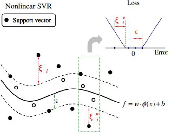
Support vector machine for regression (SVR) is a supervised learning method for the function approximation. This network, which was first introduced by Vapnik, minimizes the risk of correct classification instead of minimizing the modeling error [33]. SVR neural networks have been used in recent years for modeling several systems [34, 35]. The goal of this method is to find the optimal hyperplane in the high-dimensional feature space and use it for the function approximation in the regression problem. Vapnik’s loss function is used for the application of support vector machine in the regression problem, which is known as the 𝜀𝜀 -insensitive loss function. In other words, errors are not significant as long as they are smaller than 𝜀𝜀, but the larger values are not

allowed:

Lε�yi,f(xi)�

=� |yi−f(xi)|− ε if |yi−f(xi)|≥ ε 0 otherwise

(10)

This function creates a hyperplane 𝑓𝑓(𝑥𝑥) which has the biggest deviation 𝜀𝜀 from the actually obtained targets 𝑦𝑦_𝑖𝑖 for all training data. Suppose the training patterns(𝑥𝑥₁,𝑦𝑦₁), (𝑥𝑥₂,𝑦𝑦₂),…, (𝑥𝑥_𝑙𝑙,𝑦𝑦_𝑙𝑙), where

𝑥𝑥𝑖𝑖 ∈ 𝑅𝑅𝑛𝑛 is a feature vector,𝑖𝑖= 1,2,…,𝑙𝑙, 𝑙𝑙 is the number of training patterns, and 𝑦𝑦_𝑖𝑖 ∈ 𝑅𝑅 is the target value. Regression function of 𝑓𝑓(𝑥𝑥) can be formulated as follows:

f(x) = wT_ϕ_{(x) + b} ₍₁₁₎

Similarly, the nonlinear regression problem can be expressed schematically in Figure 4.

Figure 4. Nonlinear SVR with 𝜀𝜀-insensitive loss function [38].

where 𝜙𝜙(𝑥𝑥) indicates the nonlinear mapping function from the input space to the feature space. 𝑤𝑤 is the vector of weight coefficients, and b stands for the bias term. These parameters are estimated by minimizing the risk function with constraints as shown in the following:

ϕ(w,_ξ_{) =}1 2�|w|�

2

+ C�(ξi+ξi∗) N

i=1

(12)

� yi−< w

,_ϕ_(x_i_{) >}₋_b_{≤ ε − ξ}_i < w,_ϕ_(x_i_{) > +b}₋_y_i_{≤ ε − ξ}_i∗

ξi.ξi∗≥0

(13)

(8)

cost function measuring the empirical risk, and 𝜉𝜉_𝑖𝑖,𝜉𝜉_𝑖𝑖∗ are the slack variables used to control overfitting; the solution problem as a quadratic programing based in the Karush-Kuhn-Tucker (KKT) conditions for nonlinearly separable data could be achieved by simply preprocessing the training patterns into feature space by 𝜙𝜙(𝑥𝑥). In this state, the following equation is achieved.

f(x) =�(αi− αi∗) n

i=1

K(xi. x) + b (14)

b =_|S|1 �yi− �(αi− αi∗) n

i=1

K(xi. x) i

−sign(αi +αi∗)ε)

(15)

In the above equations, 𝛼𝛼_𝑖𝑖 and 𝛼𝛼_𝑖𝑖∗ are nonzero Lagrangian multipliers, and S denotes support vector. 𝐾𝐾(𝑥𝑥_𝑖𝑖.𝑥𝑥) is the kernel function that represents the inner product (<𝜙𝜙(𝑥𝑥𝑖𝑖),𝜙𝜙(𝑥𝑥𝑖𝑖) >). Different kernels, such as linear, polynomial, and Gaussian, may be used as kernel functions for regression; however, in this study, the Gaussian function is used as the kernel [36].

3. Results and discussion

3.1. Data collection and preprocessing

In order to create a comprehensive model for the solubility prediction, a large experimental dataset has to be collected. In this study, the experimental aqueous solubility data of 666 different pharmaceutical compounds [37–39] and solubility data of 712 pharmaceutical compound in organic solvents [39–43] were collected from different standard sources. The chemical structures of all pharmaceutical compounds and organic solvents of the dataset were presented according to the first order functional groups of the Marrero and Gani method [44]. The dataset consisted of 78 functional groups for the aqueous systems and

65 structural groups for the organic solvents, respectively. The input variables for the solubility prediction consisted of the melting point (MP), molecular weight (MW), temperature (T), and the number of functional groups forming the molecule of a pharmaceutical compound and the organic solvents (𝑁𝑁_𝑖𝑖).

All data were divided into three groups of training, validation, and testing. The training data consisting of (70 %) of all data were used to construct the structure of the ANN and update the weight vector and biases. The validation data consisting of (10 %) of the total data were used to validate the generalized feature of the model. The testing data consisting of (20 %) of data were used to check the model performance [45]. The data were normalized between [−1 +1] due to Eq. (16):

pn.i= 2∗_ppi−pmin

max−pmin−1 (16)

where 𝑝𝑝_𝑛𝑛_._𝑖𝑖 stands for the normalized value of input variable 𝑝𝑝_𝑖𝑖; 𝑝𝑝_{𝑚𝑚𝑖𝑖𝑛𝑛} and p_max stand for the minimum and maximum values, respectively [24].

The next calculation step is to find a relationship between the chemical functional groups and the solubility data using the collected dataset. For this purpose, the multilayer perceptron neural network, radial basis function network, and the support vector machine for regression were applied to the collected dataset.

3.2. Model development

3.2.1. The optimized MLP network configuration

(9)

and the transfer function in each layer by trial and error according to the minimization of an objective function, which is the Average Absolute Relative Deviation (AARD) between the output of the developed MLP and the target values for the presented dataset. This optimization process is performed during the training process with the Levenberg-Marquardt (LM) and particle swarm optimization algorithms to determine the weight matrix and bias vector.

To avoid the overfitting of the neural network, the number of the neurons in the

hidden layer of the network was limited to 20. The MLP model was trained with different transfer functions, training algorithms, and the variable number of neurons in the hidden layers. Finally, the MLP models with the 81-14-1 and 68-81-14-1 architectures (81 and 68 neurons in the input layer, 14 neurons in the hidden layer, and 1 neuron in the output layer) with the tan-sigmoid transfer function showed the least AARD value for water and organic solvents. The results are presented in Figure 5.

Figure 5. AARD versus the number of neurons in the second hidden layer for (a) water and (b) organic solvents.

The predicted values for the solubility in water and organic solvents using the trained

MLP model with Levenberg–Marquardt (LM) and particle swarm optimization (PSO)

0 2 4 6 8 10 12 14 16 18 20

number of neuron

0.4 0.6 0.8 1 1.2 1.4 1.6 1.8 2 2.2

AARD

AARDtr

AARDts

AARDval

a

0 2 4 6 8 10 12 14 16 18 20

number of neuron

0 1 2 3 4 5 6 7 8

AARD

AARDtr

AARDts

AARDval

(10)

algorithms versus the experimental value of test data are compared, as shown in Figures 6 and 7.

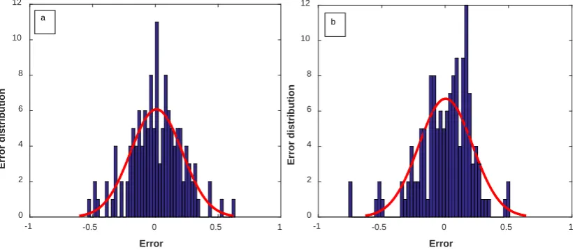
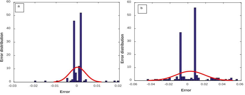
The error distribution of the optimized

MLP-LM and MLP-PSO models for water and organic solvents is shown in Figures 8 and 9 to detect the accuracy of different MLP models.

Figure 3. Regression graph for pharmaceutical solubility in (a) water and (b) organic solvents for test data by the optimized MLP-LM model.

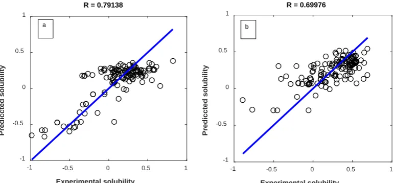
Figure 4. Regression graph for pharmaceutical solubility in (a) water and (b) organic solvents for test data by the optimized MLP-PSO model.

-1 -0.5 0 0.5 1

Experimental solubility -1

-0.5 0 0.5 1

Prediccted solubility

R = 0.8972

-1 -0.5 0 0.5 1

-0.5 0 0.5

1

R = 0.81719

a _b

-1 -0.5 0 0.5 1

-0.5 0 0.5 1

R = 0.79138

-1 -0.5 0 0.5 1

-0.5 0 0.5 1

R = 0.69976

(11)

Iranian Journal of Chemical Engineering, Vol. 16, No. 1 (Winter 2019) 93 Figure 5. Histogram of error distribution for pharmaceutical solubility in (a) water and (b) organic

solvents for test data by the optimized MLP-LM model.

Figure 6. Histogram of error distribution for pharmaceutical solubility in (a) water and (b) organic solvents for test data by the optimized MLP-PSO model.

3.2.2. The optimized RBF network configuration

The structure of the RBF neural network was created and trained using a newrb function in Matlab 2015. To find the optimized RBF model, it is necessary to obtain two main

parameters. These two main parameters include the number of maximum hidden neurons and the spread, which have to be calculated by the trial-and-error approach. After finding the optimized values of these parameters, the best performance of the

-0.5 0 0.5 1

Error 0

5 10 15 20

Error distribution

-1 -0.5 0 0.5 1

Error 0

5 10 15 20

a

b

-1 -0.5 0 0.5 1

Error 0

2 4 6 8 10 12

-1 -0.5 0 0.5 1

Error 0

2 4 6 8 10 12

a

(12)

network was obtained by minimizing the Average Absolute Relative Deviation (AARD). The optimal value of the spread and maximum neuron numbers according to AARD were equal to 80 and 30 for water and organic solvents, respectively. The predicted values of solubility for water and organic

solvents are presented versus the experimental values of the test data in Figure 10.

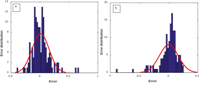
The error distribution of the optimized RBF model for water and organic solvents is shown in Figure 11 to show the accuracy of the RBF model.

Figure 7. Regression graph for pharmaceutical solubility in (a) water and (b) organic solvents for test data by the optimized RBF model.

Figure 8. Histogram of error distribution for pharmaceutical solubility in (a) water and (b) organic solvents for test data by the optimized RBF model.

-1 -0.5 0 0.5 1

Experimental solubility

-1 -0.5

0 0.5

1

R = 0.87061

-1 -0.5 0 0.5 1

-1 -0.5

0 0.5

1

R = 0.77824

a _b

-0.5 0 0.5 1

Error

0 2 4 6 8 10 12 14

-1 -0.5 0 0.5

Error

0 5 10 15 20

a

(13)

Iranian Journal of Chemical Engineering, Vol. 16, No. 1 (Winter 2019) 95 3.2.3. The proposed SVR-PSO model

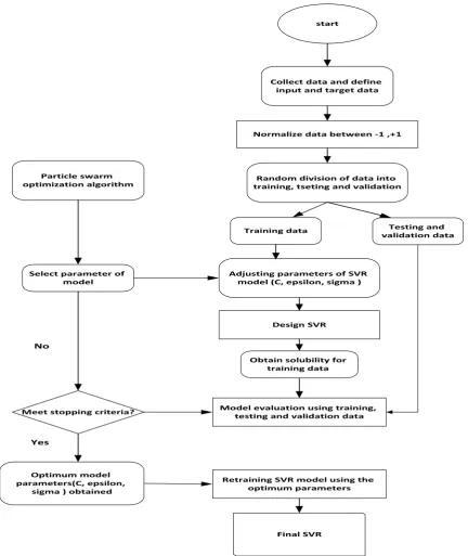
In this study, the support vector regression method combined with particle swarm optimization was used to develop a neural model for the prediction of pharmaceutical solubility. A Gaussian function was used as the kernel function with a spread parameter, called sigma. The first step of designing an SVR model is to obtain the parameters (C,

epsilon) and the RBF spread parameter. To search for the optimum value of these parameters, the particle swarm optimization algorithm based on the Average Absolute Relative Deviation as the objective function was used. This algorithm is shown in the flowchart presented in Figure 12. The optimum values of the parameters for the current dataset are presented in Table 1.

Figure 9. Flowchart of SVR-PSO model.

start

Normalize data between -1 ,+1 Collect data and define

input and target data

Random division of data into training, tseting and validation

Testing and validation data Training data

Adjusting parameters of SVR model (C, epsilon, sigma )

Design SVR

Obtain solubility for training data

Meet stopping criteria? Select parameter of

model Particle swarm optimization algorithm

Optimum model parameters(C, epsilon,

sigma ) obtained

Model evaluation using training, testing and validation data

Retraining SVR model using the optimum parameters

Final SVR

(14)

96 Iranian Journal of Chemical Engineering, Vol. 16, No. 1 (Winter 2019) Table 1

Optimum parameters for the SVR-PSO model.

solvent C Epsilon Sigma

water 195.0803 0.001274 0.246

Organic solvents 425.26 0.00793 0.298

The predicted solubility values for water and organic solvents using the optimum SVR-PSO model are compared with the testing experimental data in Figure 13.

The error distribution of the optimized SVR-PSO model for water and organic solvents is shown in Figure 14.

Figure 10. Regression graph for pharmaceutical solubility in (a) water and (b) organic solvents for test data by the optimized SVR-PSO model.

Figure 11. Histogram of error distribution for pharmaceutical solubility in (a) water and (b) organic solvents for test data by the optimized SVR-PSO model.

-1 -0.5 0 0.5 1

-1 -0.5

0 0.5

1

R = 0.99993

-0.5 0 0.5 1

-0.5 0 0.5

1

R = 0.998

b a

-0.03 -0.02 -0.01 0 0.01 0.02

Error

0 10 20 30 40 50 60

-0.06 -0.04 -0.02 0 0.02 0.04 0.06

Error

0 10 20 30 40 50 60

a

(15)

Iranian Journal of Chemical Engineering, Vol. 16, No. 1 (Winter 2019) 97 3.2.4. The statistical measures for the

model performance

In order to compare the accuracy of prediction models, three different statistical measures of Average Absolute Relative Deviation (AARD), correlation factor (𝑅𝑅), and Root Mean Squared Error (RMSE) were used. These parameters are calculated as follows:

𝐴𝐴𝐴𝐴𝑅𝑅𝐴𝐴= ��𝑌𝑌𝑝𝑝𝑝𝑝𝑝𝑝𝑝𝑝(_𝑌𝑌𝑖𝑖)− 𝑌𝑌𝐸𝐸𝐸𝐸𝑝𝑝(𝑖𝑖)�

𝐸𝐸𝐸𝐸𝑝𝑝(𝑖𝑖) 𝑁𝑁

𝑖𝑖=1

(17)

𝑅𝑅=�1− �∑ �𝑌𝑌𝑝𝑝𝑝𝑝𝑝𝑝𝑝𝑝(𝑖𝑖)− 𝑌𝑌𝐸𝐸𝐸𝐸𝑝𝑝(𝑖𝑖)�

2 𝑁𝑁

𝑖𝑖=1

∑ �𝑌𝑌𝑁𝑁𝑖𝑖=1 exp(𝑖𝑖)�2

� (18)

𝑅𝑅𝑅𝑅𝑅𝑅𝑅𝑅= 1

𝑁𝑁 �(

𝑌𝑌𝑝𝑝𝑝𝑝𝑝𝑝𝑝𝑝(𝑖𝑖)− 𝑌𝑌𝐸𝐸𝐸𝐸𝑝𝑝(𝑖𝑖)

𝑌𝑌𝐸𝐸𝐸𝐸𝑝𝑝(𝑖𝑖) ) 𝑁𝑁

𝑖𝑖=1

(19)

In these equations, N is the number of input data, and 𝑌𝑌_{𝑝𝑝𝑝𝑝𝑝𝑝𝑝𝑝}(𝑖𝑖) and 𝑌𝑌_{𝐸𝐸𝐸𝐸𝑝𝑝}(𝑖𝑖) are the

predicted and actual output values of the 𝑖𝑖𝑡𝑡ℎ input dataset, respectively [25].

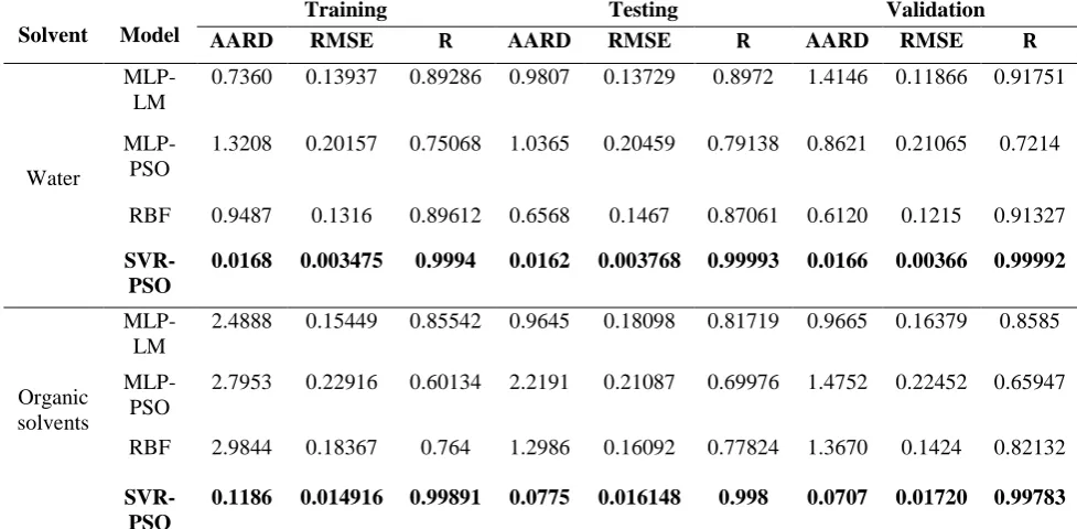
In order to compare the accuracy of the developed models, the statistical parameters for training, testing, and validation data were calculated, as presented in Table 2. The results of this table showed that the SVR-PSO model was more accurate than the MLP and RBF models.

Table 2

Statistical parameters of the developed models.

Solvent Model

Training Testing Validation

AARD RMSE 𝐑𝐑 AARD RMSE 𝐑𝐑 AARD RMSE 𝐑𝐑

Water

MLP-LM

0.7360 0.13937 0.89286 0.9807 0.13729 0.8972 1.4146 0.11866 0.91751

MLP-PSO

1.3208 0.20157 0.75068 1.0365 0.20459 0.79138 0.8621 0.21065 0.7214

RBF 0.9487 0.1316 0.89612 0.6568 0.1467 0.87061 0.6120 0.1215 0.91327

SVR-PSO

0.0168 0.003475 0.9994 0.0162 0.003768 0.99993 0.0166 0.00366 0.99992

Organic solvents

MLP-LM

2.4888 0.15449 0.85542 0.9645 0.18098 0.81719 0.9665 0.16379 0.8585

MLP-PSO

2.7953 0.22916 0.60134 2.2191 0.21087 0.69976 1.4752 0.22452 0.65947

RBF 2.9844 0.18367 0.764 1.2986 0.16092 0.77824 1.3670 0.1424 0.82132

SVR-PSO

0.1186 0.014916 0.99891 0.0775 0.016148 0.998 0.0707 0.01720 0.99783

4. Conclusions

Four intelligence models, namely MLP, MLP-PSO, RBF, and SVR-PSO, based on the group contribution, and neural networks were developed in order to present a comprehensive and accurate model for the prediction of pharmaceutical solubility in

(16)

(PSO) training algorithm showed the AARD equal to 1.3208 and 2.7953 for the solubility of pharmaceuticals in water and organic solvents, respectively. Optimum RBF network architecture was created with 30 neurons and a spread equal to 80. The AARD of this model was equal to 0.6568 for pharmaceutical solubility in water and 1.2986 for pharmaceutical solubility in organic solvents. PSO algorithm was used to determine the cost function and the C, epsilon, and sigma parameters in the SVR model. The AARD of the SVR model optimized by the PSO algorithm was equal to 0.0162 and 0.0775 for water and organic solvents, respectively. The cross plot and error distribution figures showed that the SVR-PSO model with RBF kernel function predicted the pharmaceutical solubility better than MLP-LM, MLP-PSO, and RBF models. These results showed that the predictions of SVR-PSO were the most comprehensive and accurate.

References

[1] Siepmann, J. and Siepmann, F.,

“Mathematical modeling of drug dissolution”, Int. J. Pharm., 453, 12 (2013).

[2] Inczedy, J., Lengyel, T. and Ure, A. M., Compendium of analytical nomenclature, 3rd edition, Blackwell Science, USA, (1998).

[3] Prausnitz, J. M., Lichtenthaler, R. N., de Azevedo, E. G. and Rowlinson, J., Molecular thermodynamics of fluid-phase equilibria, Pearson Education, USA, (1998).

[4] Delaney, J. S., “Predicting aqueous

solubility from structure”, Drug Discov. Today, 10, 289 (2005).

[5] Babu, V. R., Areefulla, S. H. and

Mallikarjun, V., “Solubility and

dissolution enhancement: An overview”, J. Pharm. Res., 3, 141 (2010).

[6] Savjani, K. T., Gajjar, A. K. and Savjani, J. K., “Drug solubility: Importance and enhancement techniques”, ISRN Pharm.,

2012, 195727 (2012).

[7] Feng, L., van Hullebusch, E. D.,

Rodrigo, M. A., Esposito, G. and Oturan, M. A., “Removal of residual

anti-inflammatory and analgesic pharmaceuticals from aqueous systems by electrochemical advanced oxidation processes: A review”, Chem. Eng. J.,

228, 944 (2013).

[8] Lindenberg, C., Kråttli, M., Cornel, J.

and Mazzotti, M., “Design and

optimization of a combined

cooling/antisolvent crystallization

process”, Cryst. Growth Des., 9, 1124 (2009).

[9] Blanchard, L. a. and Brennecke, J. F., “Recovery of organic products from ionic liquids using supercritical carbon dioxide”, Ind. Eng. Chem. Res., 40, 2550 (2001).

[10]Crerar, D. A. and Anderson, G. M., “Solubility and solvation reactions of quartz in dilute hydrothermal solutions”, Chem. Geol., 8, 107 (1971).

[11]Gmehling, J. G., Anderson, T. F. and Prausnitz, J. M., “Solid-liquid equilibria

using UNIFAC”, Ind. Eng. Chem.

Fundam., 17, 269 (1978).

[12]Feelly Ruether, G. S., “Modeling the solubility of pharmaceuticals in pure solvents and solvent mixtures for drug process design”, J. Pharm. Sci., 98, 4205 (2009).

(17)

mixed solvent mixtures for organic

pharmacological compounds with

COSMO-based thermodynamic

methods”, Ind. Eng. Chem. Res., 47, 1707 (2008).

[14]Zhao, Y., Wu, Z., Liu, W. and Pei, X., “A new theoretical model for predicting the solubility of solid solutes in different solvents”, Fluid Phase Equilib., 412, 123 (2016).

[15]Gharagheizi, F., “Representation/

prediction of solubilities of pure compounds in water using artificial neural network-group contribution method”, J. Chem. Eng. Data, 56, 720 (2011).

[16]Yalkowsky, S. H. and Valvani, S. C., “Solubility and partitioning, I: Solubility of nonelectrolytes in water”, J. Pharm. Sci., 69, 912 (1980).

[17]Ruelle, P. and Kesselring, U. W., “Solubility predictions for solid nitriles and tertiary amides based on the mobile

order theory”, Pharm. Res., 11, 201

(1994).

[18]Abraham, M. H. and Le, J., “The

correlation and prediction of the solubility of compounds in water using an amended solvation energy relationship”, J. Pharm. Sci., 88, 868 (1999).

[19]Klamt, A., Eckert, F., Hornig, M., Beck, M. E. and Brger, T., “Prediction of aqueous solubility of drugs and pesticides with COSMO-RS”, J. Comput. Chem., 23, 275 (2002).

[20]Wang, J., Krudy, G., Hou, T., Zhang, W., Holland, G. and Xu, X. J., “Development of reliable aqueous solubility models and their application in druglike analysis”, J. Chem. Inf. Model., 47, 1395 (2007). [21]Huuskonen, J., “Estimation of aqueous

solubility for a diverse set of organic

compounds based on molecular

topology”, J. Chem. Inf. Comput. Sci.,

40, 773 (2000).

[22]Hou, T. J., Xia, K., Zhang, W. and Xu, X. J., “ADME evaluation in drug discovery: 4. Prediction of aqueous solubility based on atom contribution approach”, J. Chem. Inf. Comput. Sci.,

44, 266 (2004).

[23]Gharagheizi, F., Eslamimanesh, A.,

Mohammadi, A. H. and Richon, D., “Determination of critical properties and acentric factors of pure compounds using the artificial neural network group contribution algorithm”, J. Chem. Eng. Data., 56, 2460 (2011).

[24]Chen, G., Luo, X., Zhang, H., Fu, K.,

Liang, Z., Rongwong, W.,

Tontiwachwuthikul, P. and Idem, R., “Artificial neural network models for the prediction of CO2 solubility in aqueous

amine solutions”, Int. J. Greenh. Gas

Control., 39, 174 (2015).

[25]Tatar, A., Naseri, S., Bahadori, M., Hezave, A. Z., Kashiwao, T., Bahadori, A. and Darvish, H., “Prediction of carbon dioxide solubility in ionic liquids using MLP and radial basis function (RBF) neural networks”, J. Taiwan Inst. Chem. Eng., 60, 151 (2016).

[26]Mehdizadeh, B. and Movagharnejad, K., “A comparison between neural network method and semi empirical equations to predict the solubility of different compounds in supercritical carbon dioxide”, Fluid Phase Equilib., 303, 40 (2011).

[27]Graupe, D., Principles of artificial neural networks, World Scientific, Singapore, (2013).

(18)

swarm optimization”, Proceedings of IEEE Int. Conf. Neural Networks, Perth, WA, Australia, 4, pp. 1942–1948 (2002).

[29]Haykin, S. S., Neural networks and

learning machines, 3rd Edition, USA, (2009).

[30]Broomhead, D. S. and Lowe, D., “Radial basis functions, multi-variable functional interpolation and adaptive networks”, DTIC Document, (1988).

[31]Mustafa, M. R., Rezaur, R. B., Rahardjo, H. and Isa, M. H., “Prediction of pore-water pressure using radial basis function neural network”, Eng. Geol., 135–136, 40 (2012).

[32]Shen, W., Guo, X., Wu, C. and Wu, D., “Forecasting stock indices using radial basis function neural networks optimized by artificial fish swarm algorithm”, Knowledge-Based Syst., 24, 378 (2011). [33]Vladimir, V. N. and Vapnik, V., The

nature of statistical learning theory, Springer-Verlag, Berlin, Germany, (1995).

[34]Kazem, A., Sharifi, E., Hussain, F. K., Saberi, M. and Hussain, O. K., “Support vector regression with chaos-based firefly algorithm for stock market price forecasting”, Appl. Soft Comput., 13, 947 (2013).

[35]Yu, P. S., Chen, S. T. and Chang, I. F., “Support vector regression for real-time flood stage forecasting”, J. Hydrol., 328, 704 (2006).

[36]Smola, A. J. and Schölkopf, B., “A tutorial on support vector regression”, Stat. Comput., 14, 199 (2004).

[37]Yalkowsky, S. H., He, Y. and Jain, P., Handbook of aqueous solubility data, 2nd ed., CRC Press, USA, (2010).

[38]Ribeiro Neto, A. C., Pires, R. F., Malagoni, R. A. and Franco, M. R., “Solubility of vitamin C in water, ethanol, propan-1-ol, water + ethanol, and water + propan-1-ol at (298.15 and 308.15) K”, J. Chem. Eng. Data, 55, 1718 (2010).

[39]Pobudkowska, A., Domańska, U. and

Jurkowska, B. A., “Solubility of

pharmaceuticals in water and alcohols”, Fluid Phase Equilib., 392, 56 (2015). [40]Wenju, L., Leping, D., Black, S. and

Hongyuan, W., “Solubility of

carbamazepine (form III) in different solvents from (275 to 343) K”, J. Chem. Eng. Data, 53, 2204 (2008).

[41]Li, Q. S., Li, Z. and Wang, S.,

“Solubility of trimethoprim (TMP) in different organic solvents from (278 to 333) K”, J. Chem. Eng. Data, 53, 286 (2008).

[42]Jouyban, A., Handbook of solubility data for pharmaceuticals, CRC Press, USA, (2009).

[43]Wang, L., Du, C., Wang, X., Zeng, H., Yao, J. and Chen, B., “Solubilities of phosphoramidic acid, N-(phenylmethyl)-, diphenyl ester in selected solvents”, J. Chem. Eng. Data, 60, 1814 (2015). [44]Marrero, J. and Gani, R.,

“Group-contribution based estimation of pure

component properties”, Fluid Phase

Equilib., 183–184, 183 (2001).

[45]Agirre-Basurko, E., Ibarra-Berastegi, G. and Madariaga, I., “Regression and multilayer perceptron-based models to forecast hourly O3 and NO2 levels in the