Volume 61, 2019, Pages 62–102
ARCH19. 6th International Workshop on Applied Verification of Continuous and Hybrid Systems
ARCH-COMP19 Category Report:
Stochastic Modelling
Alessandro Abate
1, Henk Blom
2, Nathalie Cauchi
1, Kurt Degiorgio
4, Martin
Fr¨
anzle
5, Ernst Moritz Hahn
6, Sofie Haesaert
3, Hao Ma
2, Meeko Oishi
12, Carina
Pilch
9, Anne Remke
9, Mahmoud Salamati
10, Sadegh Soudjani
7, Birgit van
Huijgevoort
3, and Abraham P. Vinod
111
University of Oxford, Department of Computer Science, Oxford, [email protected] 2
Delft University of Technology, Delft, The Netherlands and National Aerospace Laboratory, Amsterdam, The Netherlands{Henk.Blom,Hao.Ma}@nlr.nl
3
TU Eindhoven, Eindhoven, The Netherlands{S.Haesaert, b.c.v.huijgevoort}@tue.nl 4 Diffblue Ltd, Oxford, UK
Oldenburg University, Oldenburg, [email protected] 6 University of Liverpool, Liverpool, UK[email protected]
7
School of Computing, Newcastle University, UK,[email protected] 8 University of M¨unster, Germany{carina.pilch, anne.remke}@uni-muenster.de
9
Max Planck Institute for Software Systems, [email protected] 10
University of New Mexico, Department of Electrical and Computer Engineering, New Mexico, USA{oishi}@unm.edu
11
The University of Texas at Austin, Department of Aerospace Engineering and Engineering Mechanics, Texas, [email protected]
Abstract
This report presents the results of a friendly competition for formal verification and pol-icy synthesis of stochastic models. It also introduces new benchmarks within this category, and recommends next steps for this category towards next year’s edition of the competi-tion. The friendly competition took place as part of the workshop Applied Verification for Continuous and Hybrid Systems (ARCH) in Spring 2019.
1
Introduction
provide a set of benchmarks which we aim to push forward the development of current and future tools. To establish further trustworthiness of the results, the code describing the benchmarks together with the code used to compute the results is publicly available at
gitlab.com/goranf/ARCH-COMP.
This report summarizes results obtained in the 2019 friendly competition of the ARCH workshop1 for thestochastic modelling group. In this edition, we have divided our work over
two targets:
1. the generation of new benchmarks, comprising different model structures and dealing with diverse applications and tasks to be solved; and
2. the friendly competition, run over previously identified benchmarks.
We have additionally initiated a discussion about setting up a formal language for stochastic models (or a subset thereof). This is specifically seen within the heated tank benchmarks, were different formalisms are collated and key differences are identified. We will leave this as future work (see relevant final section).
The tools and frameworks used are (in alphabetical order): (, δ)Abstraction,FAUST2, HYPEG,LyapMMC,Modest Toolset,SReachTools,StocHy,SDCPN. We emphasise in particular the introduction of four new tools and/or frameworks. All the tools and frameworks have been compiled into docker format (a container software), which allows for easier readability evaluation of the generated results together with the sharing of the tools themselves to both the ARCH and the wider research community.
This report has the following structure. Section2 provides a short overview of the partic-ipating tools and frameworks. Section3 presents a set of new benchmark descriptions, which include a discussion of the individual models syntax and semantics, and a presentation of the specifications of interest. Next, in Section4we present the results of the friendly competition where the participating tools or algorithmic frameworks that are used to solve instances of the benchmarks from last year’s edition. We identify key challenges and discuss future plans in Section5.
2
Participating Tools & Frameworks
The tools and frameworks used in the category Stochastic Modelling are introduced next, or-ganised in alphabetical order.
2.1
Tools
FAUST2 The toolFormal Abstractions of Uncountable-STate STochastic processes(
FAUST2) [48] generates formal abstractions of discrete-time Markov processes (dtMP) defined over con-tinuous state spaces. The dtMP model is abstracted into a finite-state Markov chain or a Markov decision process. The abstract model is formally put in relationship with the concrete dtMP via a user-defined maximum threshold on the approximation error introduced by the ab-straction procedure. FAUST2allows exporting the abstract model to well-known probabilistic model checkers, such as PRISM [36] or STORM [17]. Alternatively, it can handle internally
the computation of basic PCTL properties (e.g. safety or reach-avoid) over the abstract model, and refine the outcomes over the concrete dtMP via a quantified error that depends on the abstraction procedure and the given formula. The toolbox relies on approaches developed and adapted to different classes of systems and under different assumptions [46,43,47,44,45]. The toolbox is available athttps://sourceforge.net/projects/faust2/
HYPEG The Java-based libraryHYPEG[38] is a simulator for hybrid Petri nets with general transitions (HPnGs) [27] which combine discrete and continuous components with a possibly large number of random variables, whose stochastic behavior follows arbitrary probability dis-tributions. HYPEG uses time-bounded discrete-event simulation and well-known Statistical Model Checking techniques to verify complex properties, including time-bounded reachabil-ity [39]. These techniques comprise several hypothesis tests as well as different approaches for the computation of confidence intervals. In the latest version of HYPEG, continuous behavior that can be expressed by systems of ordinary differential equations can be simulated using an approximative approach [37], whereas piecewise-linear continuous behavior is simulated without approximation.
LyapMMC Using the tool Lyapanov-based Markov Model Checker (LyapMMC), verification problems over continuous-time Markov chains (ctmc) and continuous-time Markov decision processes (ctmdp) can be solved efficiently([40]). The core verification problem forctmcs and ctmdps is time-bounded reachabilty. It can be computed by numerically solving a characteristic linear dynamical system but the procedure is computationally expensive. We take a control-theoretic approach and propose a reduction technique that finds another dynamical system of lower dimension (number of variables), such that numerically solving the reduced dynamical system provides an approximation to the solution of the original system with guaranteed error bounds.
Modest Toolset The Modest Toolset [32] supports the modelling and analysis of hy-brid, real-time, distributed and stochastic systems. A modular framework centred around the stochastic hybrid automata formalism [31] and supporting the JANI specification [9], it provides a variety of input languages and analysis backends. The modelling formalism at the core of the Modest Toolsetis the model of networks of stochastic hybrid automata (SHA), which com-bine nondeterministic choices, continuous system dynamics, stochastic decisions and timing, and real-time behaviour, including nondeterministic delays. A wide range of well-known and extensively studied formalisms in modelling and verification can be seen as special cases of SHA e.g. STA (stochastic timed automata), PTA (probabilistic timed automata) and MDP (Markov decision processes). The toolset can can be obtained fromhttp://www.modestchecker.net/. For the experiments on the Heated Tank benchmark, we have used the Modest Toolset’s simulator “modes” [8] and its support for rare event simulation based on importance splitting with the fixed effort method (using 64 child runs for each fixed effort run) [7].
geometry for a grid-free and scalable computation of the stochastic reach sets as well as con-troller (open-loop, affine feedback, and set-based) synthesis [25,53,54,56,41]. The toolbox is available athttps://unm-hscl.github.io/SReachTools/.
StocHy [12] is a software tool for the quantitative analysis of discrete-timestochastic hybrid systems (shs). StocHy accepts a high-level description of stochastic models and constructs an equivalent shsmodel. The tool allows to (i) simulate the shsevolution over a given time horizon; and to automatically construct formal abstractions of theshs- these are grounded on interval MDPs [13] and show the benefit of providing scalability and tighter error bounds than cognate approaches [11]. Abstractions are then employed for (ii) formal verification or (iii) control (policy, strategy) synthesis. StocHyallows for modular modelling, and has separate simulation, verification and synthesis engines, which are implemented as independent libraries. This allows for libraries to be easily used and for extensions to be easily built. The tool is implemented inc++ and employs manipulations based on vector calculus, the use of sparse matrices, the symbolic construction of probabilistic kernels, and multi-threading. StocHyis available atwww.gitlab.com/natchi92/StocHy.
2.2
Frameworks
(, δ) Abstraction Based on the papers [28,29, 42], this software library uses code snippets and algorithms to compute two precision parameters (, δ), which allow bounding the deviations between models in both the output signals () and the transition probabilities (δ). The obtained abstract models, either with deterministic continuous states or with stochastic finite states, are then employed in probabilistic model checking.
SDCPN modelling & Rare Event simulation Stochastically and Dynamically Coloured Petri Nets (SDCPN) [18, 19, 20, 21] have been developed in support of the compositional modelling of continuous-time Piecewise Deterministic Markov Processes [16] and Generalized Stochastic Hybrid Processes [10]. In combination with conditional and rare event MC sim-ulation, SDCPN modelling has successfully been applied for the quantitative risk modelling and assessment of future air traffic management designs, e.g. [4]. The SDCPNframework is suitable for all versions of the Heated Tank benchmark. For rare event simulation it can con-duct straightforward Monte Carlo (MC) simulation as well as the Interacting Particle System (IPS) acceleration approach [4,5,14] for reach probability evaluation of Generalised Stochastic Hybrid Processes.
3
New benchmarks
We present a set of new benchmarks (alphabetically ordered), in this section. The benchmarks highlight different tasks and modelling complexities that are not currently handled within the current benchmarks. For additional benchmarks please refer to last year’s report [1] and to [42].
3.1
Networked automation system [
26
]
Figure 1: A networked automation system from [26].
transportation unit which controls the speed of the conveyor belt transporting the workpiece. The PLC can set the deceleration of the belt via network messages to the transportation unit, but cannot determine the position of the object unless it hits two sensors SA and SB close to the drilling position. The sensors are connected to the IO card of the PLC over the network. When the object reaches sensor SA, the PLC reacts with sending a command to the transportation unit that forces it to decelerate to slow speed. Likewise, the transportation unit is asked to decelerate to stand-still when the PLC notices that SB has been reached. The goal is that the object halts close to the drilling position despite the uncontrollable latencies in the communication network. The parameters of the system are adopted from [26] as far as indicated. Thus, one length unit (lu) is 0.01 mm, and one time step (ts) is 1 ms. The positions of SA and SB are 699 lu and 470 lu, respectively, while the acceptable drilling position are between 100 lu and 0 lu. The initial speed of the object is 24 lu/ts and the slow speed is 4 lu/ts; the decelerations for the two types of speed changes at SA and SB are 2 lu/ts2 and 4 lu/ts2, respectively. The network routing time is determined stochastically, needing 1 ts for delivery with probability 0.9 and 2 ts with probability 0.1. The cycle time of the PLC-IO card is 10 ts, while the cycle time of the PLC itself is 7 ts. Please note that these cycle times are not multiples of each other (in fact, even co-primal), resulting in a systematic cyclic variation of end-to-end response time of the PLC setup. The minimum sampling interval is 1 ts. Due to the initial speed of 24 lu/ts, the initial position of the object is thus equally distributed over 24 neighboring values, namely the range between 999 lu and 976 lu.
Task: Compute the probability of stopping within the region [100lu,0lu] of acceptable drilling positions.
3.2
Scheduling
Imagine a system of 16 structurally identical tasks running in sequence. Each task has a worst-case execution time (WCET) of 1 ms, with their actual run times being independent random variables featuring a triangular density, as depicted in Figure2. Each task hence has 0.25% probability of exceeding 95% of itsWCET.
Task: Compute (a conservative approximation of) the probability for the 16 tasks together exceeding 95% of their accumulatedWCETof 16 ms.
3.3
Tandem Network
WCET (1ms) density of
actual runtimes
95% WCET
0.25% 99.75%
t
Figure 2: Runtime distribution for a single task
Figure 3: A typical tandem network ([34])
In Figure3, both queuing stations have a capacity denoted bycap. The first queuing station has two phases for processing jobs, while the second queuing station has only one phase. In Figure3, different phases are indicated by circles, with their corresponding rates written inside them. Jobs arrive at the first queuing station with rateλand are processed in the first phase with rate µ1. After this phase, jobs are passed through the second phase with probability a1 and will be processed with the rateµ2before passing to the second station. Alternatively, jobs will be sent directly to the second queuing station with probabilityb1. Processing in the second station is done with the rateκ.
The tandem network can be modelled as a continuous-time Markov chain (ctmc) with a state space of size determined bycap. Given a time boundT, we seek computing the probability of reaching to the configurations in which both stations are at their full capacity (blocked state) starting from a configuration in which both stations are empty (empty state). Therefore,blocked stateis chosen as thegood(absorbing) state. First, we need to model the given tandem network as actmc. Figure4 demonstrates the correspondingctmcfor the case thatcap= 1.
The states are of the form (l1, p, l2), wherel1is the number of jobs in first station,p∈ {0,1,2} is the status of servicing in the first station (0 means that no service is going on, 1 means that a job is in the first phase,and 2 means that a job is in the second phase) and l2 indicates the number of jobs in the second station. Given higher values for cap, one can compute the correspondingctmc, modelling the original tandem network by applying the same procedure.
3.4
Water Sewage Treatment Plant
Figure 4: ctmcfor a tandem network with cap= 1 [35]
adaptation in [27]. Pumps are used to transport sewage from one tank to another and are associated with a predefined nominal rate and can be reduced for rate adaptation purposes. Pipes connect pumps and tanks and vice versa. Note that we abstract from further parameters, like e.g. the diameter of pipes and the pressure in tanks and pipes.
This system has previously been evaluated in [24], where the model is limited in the number of stochastic variables and restricted to linear continuous dynamics without diffusion. By using models that allow for diffusion stochastic differential equations, one might be able to incorporate the cleaning steps including chemicals and bacterias into the model.
Overflow tanks are used to model sedimentation tanks as can be seen in the bird’s-eye view of a sewage treatment facility in Figure 5. A sedimentation tank physically separates suspended solids from water using gravity. The process is such that the contaminated sewage containing solids enters the tank and stays there for a certain period of time, during which the solids sediment to the ground. At a certain rate the so-called sludge is removed from the bottom of the tank, while at the top of the tank the cleaned water overflows. Overflow tanks, depicted separately in Figure6b, have a certain capacity, one input and two outputs, where one corresponds to taking out the settled sludge and the other (indicated by a grey rectangle) models the overflow. The rate of the input and the sludge output are determined by the connecting pumps, while the output of the overflow is determined by the difference of the output and the input.
like sand from the water. Then the sewage flows into a large tank, where the sludge settles and where the lighter material, like oils, rise to the surface and is removed, and the remaining cleaner water overflows. The speed of the sand interceptor is abstracted through pumpTz, and the primary sedimentation tank is modelled by the overflow tankPps.
While the dirt settles at the ground, cleaned water is forwarded to the second cleaning stage. This stage consists of several phases for removing chemical and biological contaminations, modelled by a sequence of pumps and tanks, before a second sedimentation tank separates the biological material from the now environment friendly sewage water, that can safely be disposed to surface water. The second sedimentation tank is modelled by overflow placePss. The sludge that settles at the primary and secondary sedimentation tank is accumulated and forwarded to the sludge treatment stage. There it is thickened to reduce its volume for easier off-site transport. The sludge from the primary tank is pumped out and forwarded to the fresh sludge thickener. This is also modelled by an overflow place, denotedPf t. Sludge is pumped out of the tank with a small rate and discharged to the digestion tank which is considered a very large tank. The overflow is directed to the filtrate basement. The same procedure is repeated for the accumulated sludge in the second sedimentation tank. Note that we do not consider the digestion process and the transportation of the remaining material off site.
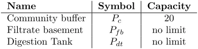
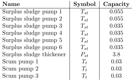
The model presented in Figure 7, is an abstraction of the real system, which consists of three parallel sand interceptor pumps and three parallel cleaning streets with several parallel primary and secondary sedimentation tanks. Moreover, fresh and surplus sludge treatment lines also consist of several parallel pumps, which are all abstracted into a single pump. Tables 1-7 provide the parameters for the entire system, where the capacity of the community buffer, the filtrate basement and the digestion tank is provided in Table1 and the rates for the Sand interceptor pumps is given in Table2. The parameters for the three different cleaning streets are provided in Tables3-5 and Tables6 and7depict the values for fresh sludge treatment and surplus sludge treatment, respectively.
(a) Primitives used in the high level description. (b) An overflow tank connected with two pumps.
Figure 6: Graphical representation.
Name Symbol Capacity
Community buffer Pc 20
Filtrate basement Pf b no limit Digestion Tank Pdt no limit
Table 1: Capacity of main tanks in the system.
Name Symbol Capacity Sand interceptor pump 1 Tz 4.7 Sand interceptor pump 2 Tz 4.7 Sand interceptor pump 3 Tz 2.6
Table 2: Rates of three different parallel sand interceptors. These are abstracted as a single pump in Figure7.
Name Symbol Capacity
Primary sedimentation tank 1 Pps 3.5 Primary sedimentation tank 2 Pps 3.5
Selector P1 1.57
Anaerobic tank P2 4.7
Aeration tank P3 5.8
Transfer rate T1, T2, T3 4
Secondary sedimentation tank 1 Pss Secondary sedimentation tank 2 Pss Secondary sedimentation tank 3 Pss Secondary sedimentation tank 4 Pss
Table 3: Cleaning street 1. This is the one considered in Figure7, with two Primary sedimen-tation tanks merged in one. Note that the capacity of the secondary sedimensedimen-tation tanks is not known to us.
Name Symbol Capacity
Primary sedimentation tank Pps 2.3
Selector P1 0.78
Anaerobic tank P2 1.15
Aeration tank P3 2.34
Transfer rate T1, T2, T3 4
Secondary sedimentation tank 1 Pss 2.3 Secondary sedimentation tank 2 Pss 2.3 Secondary sedimentation tank 3 Pss 2.3 Secondary sedimentation tank 4 Pss 2.3
Table 4: Cleaning street 2. Not considered in Figure7.
3.4.1 What to analyse?
Name Symbol Capacity
Primary sedimentation tank Pps 2.3
Selector P1 0.78
Anaerobic tank P2 11.7
Aeration tank P3 2.34
Transfer rate T1, T2, T3 4
Secondary sedimentation tank 1 Pss 2.3 Secondary sedimentation tank 2 Pss 2.3 Secondary sedimentation tank 3 Pss 2.3 Secondary sedimentation tank 4 Pss 2.3
Table 5: Cleaning street 3. Not considered in Figure7.
Name Symbol Capacity
Primary sludge pump 1 Tf t 0.3
Primary sludge pump 2 Tf t 0.3
Primary sludge pump 3 Tf t 0.3
Primary sludge pump 4 Tf t 0.35
Fresh sludge thickener Pf t 1.1
Thickened primary sludge pump 1 Tt 0.03 Thickened primary sludge pump 2 Tt 0.03 Thickened primary sludge pump 3 Tt 0.03
Table 6: Fresh sludge treatment
Name Symbol Capacity
Surplus sludge pump 1 Tst 0.055 Surplus sludge pump 2 Tst 0.055 Surplus sludge pump 3 Tst 0.035 Surplus sludge pump 4 Tst 0.035 Surplus sludge pump 5 Tst 0.035 Surplus sludge pump 6 Tst 0.035 Surplus sludge thickener Pst 3.8
Scum pump 1 Tt 0.03
Scum pump 2 Tt 0.03
Scum pump 3 Tt 0.03
Table 7: Surplus sludge treatment
is stored in the tankPo which models the amount of sewage in the street. Depending on the modelling tool which is used for the analysis of this system, one can assume a stochastic variable for the duration of rain, based on available data, and evaluate how much water is spilled in the street.
Regarding the first scenario, we have presented an analysis of how long it may continue to rain without having water in the streets in [24]. Using the logic STL [23] we formalise a property stating that the amount of water in the streets is very low until the rain stops, i.e.,
ΦA= (xPo < )U
[0,30] (m
Pn= 1), (1)
where (xPo < ) states that the amount of overflow in Place Po is smaller or equal to some , which we have chosen for computational purposes close to zero, andmPn = 1 means that the rain has stopped and we are back to normal operations. Formula ΦA is satisfied if and only if (xPo < ) (the safety condition) holds until we reachmPn= 1 (recovery condition), before the given time bound. We have chosen a time bound of 30, which is considered to be large enough for this kind of analysis.
In the second scenario, we parametrise the failure of the sand interceptor to timeα. After the occurrence of a failure, a repair crew will repair the pump with a duration distributed according to an exponential distribution, with mean 2 hours. For this case we investigated in [24] a similar formula, stating that the sand interceptor should be repaired before the street is flooded:
ΦB = (xPo <0.01)U
[α,α+30] (m
Pr = 1), (2)
where,mPr = 1, means that the sand interceptor pump is repaired. Here, we have chosen the time bound [α, α+ 30] for the Until operator, since the pump is supposed to be repaired within 30 hours after its failure. For an extensive set of results on both scenarios, we refer to [24].
4
Friendly Competition - Setup and Outcomes
4.1
Anaesthesia Model
We consider the problem of providing probabilistic guarantees of safety for the automated anaesthesia delivery problem with a human (anaesthesiologist) in the loop [22, 6, 1]. We use the well-studied multi-compartment model for delivery of Propofol (anaesthetic) in paediatrics. The depth of hypnosis can be described by the following linear dynamics
x[k+ 1] =Ax[k] +B(u[k] +σ[k]) +w[k] (3)
with state x[·] ∈ R3, automation input u[k] ∈ [0,7] ⊂
R, anaesthesiologist (human) input
σ[k] ∈ {0,30}, and input uncertainty w[k] ∼ N(0,5). See [1] for the matrices A and B
determined for a 11-year old child weighing 35 kilograms from the Paedfusor dataset [3]. In [1], we discussed a model for the human’s action (i.e., the delivery (or not) of a bolus dose of anaesthetic), as a non-deterministic, discrete-valued, discrete-time stochastic process that depends on the current state of the system, as well as the past actions of the human in a predetermined interval. Closing the loop with human control in (3) using this stochastic map results in a discrete-time stochastic hybrid system formulation. We consider the safety problem posed in [1].
Problem 4.1.1. (Stochastic viability problem)Consider a safe set
S={z∈ X : 1≤z1≤6,0≤z2≤10,0≤z3≤10}.
4.1.1 Stochastic viability with input uncertainty, but no anaesthesiologist
Figure8and Table8 discuss the results for the stochastic viability computation with no anes-thesiologist. In this case, the safety problem simplifies to stochastic viability computation of a Gaussian-perturbed linear time-invariant (lti) system with a convex safe set. In Table8we have distinguished the calculation of a lower bound on the probability of verifying the formula from the computation of the abstraction error, since some techniques are statistical in nature and cannot assess the latter.
SReachTools: We use the chance-constrained and Lagrangian (set-based) approaches avail-able in SReachTools for this problem. SReachTools does not use any abstraction, and analyzes the continuous-state problem directly.
In the chance-constrained approach, the convexity of the stochastic viability set is utilized to construct a polytopic innerapproximation via ray shooting [56]. For the easy of computation of the rays, we fixedx3[0] as it has slow dynamics.
For the Lagrangian approach, we use the notion of disturbance-minimal safe set. Recall that the computation of disturbance-minimal safe set (set of initial states from which a controller exists that is safedespite all disturbances) can be obtained using computational geometry [25]. Using the stochasticity of the disturbance, we compute a subset of the disturbance, which is guaranteed to provide an innerapproximation of the stochastic viability set. This approach does not require fixingx3[0].
StocHy: For this benchmark model, both abstraction techniques found withinStocHycan be directly used with no need for tailoring whatsoever. With the first abstraction technique (leveraging anmdp), theltiis abstracted into a Markov decision process by gridding the state-space depending on the required abstraction error and the underlying Lipschitz constants (hs) of the continuous transition kernels. (This abstraction technique corresponds to the methods used inFAUST2.) For the second technique (leveraging an imdpand native toStocHy), the ltiis abstracted into an Interval Markov decision process. In this case, the error between the original system and the abstraction is embedded within the model structure resulting in tighter error bounds when compared to the mdpmethod. For imdp, the abstraction error is defined as the = ˆp(q)−pˇ(q), where ˆp(q) and ˇp(q) correspond to the upper and lower probability bounds for each state in the imdp. In contrast for the mdp method, the N-step abstraction error corresponds to =hsδL(A) where δ is the max diameter of partition and L(A) is the volume of set.
We perform the analysis using both abstraction methods, and
• fixingx3[0] = 5,
• maintaining all three continuous variables.
When abstracting the model using themdpmethod, the control action space is discretised into three values, u= 0, u= 3.5, u= 7. Whereas, due to the little effect the control actions have over the N = 10 time horizon, for the imdp we fixu= 7. Also, note that when gridding the state-space to generate theimdp for the three dimensional model, x1 and x2 where coarsely gridded due the slow dynamics ofx3 which was seen to have small effect on the satisfaction of the safety property.
Backwards reachability: Due to the small noise signal, gridding might not be neces-sary. This conclusion is drawn based on the same reasoning and computations as described in Section B.0.1. Therefore, the noise is truncated, where the error, denoted with δ, is cho-sen equal to δ = 0.0001. This yields the Gaussian realizations w1, w2, w3 to be limited to
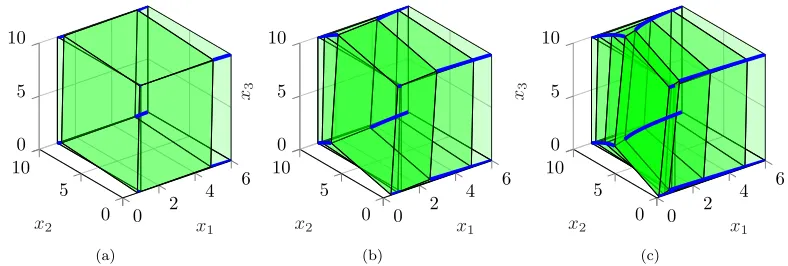
Figure 8: Stochastic viability set (initial states with safety probability of at least α= 0.99). The plot on the left fixesx3[0] = 5, and the one on the right shows the Lagrangian (set-based) underapproximation for the entire state space, obtained usingSReachTools. Compute times are given in Table8. Code available athttps://doi.org/10.24433/CO.3325937.v1.
Figure 9: The lower probability of satisfying safety property whenx3[0] = 5 is fixed and policy is generated using StocHy via abstractions into imdp. The associated computational times are given in Table8.
˜
M with truncated noise, is approximately bisimilar to the original modelM. This is denoted as ˜
M ≡=0
δ=1.00e−04M. Next, a backwards reachability computation is performed using the Multi-Parametric toolbox [33] in Matlab. After every step, the 3-dimensional polyhedron noise is subtracted. The resulting intitial set for which you will stay within the safe set is given in Figure 10. Due to the trunaction of the noise, the probability of staying in the safe set with this initial set equals (1−δ)10= 0.999.
4.1.2 Stochastic viability with anaesthesiologist, but no uncertainty
Consider inputs (v[k], σ[k])∈ {0,7} × {0,30}, respectively, enumerated as a, b, c, andd. When applied as a constant input, for the (0,0) input (a) the systems behaviour becomes autonomous. Similarly for the (7,0) input (b), the system is only affected by the control input and not by the anaesthesiologist. In contrast, inputs (7,30)cand (0,30)dreflect the (unrealistic) cases where the anaesthesiologist continuously applies a bolus dosage. Neglecting the low noise disturbance
Figure 10: Stochastic viability set (with probability 0.999) computed using −δabstraction. 0 2 4 6 0 5 10 0 5 10 x1 x2 x3 (a) 0 2 4 6 0 5 10 0 5 10 x1 x2 x3 (b) 0 2 4 6 0 5 10 0 5 10 x1 x2 x3 (c)
Figure 11: Forward reach sets for inputa are given for k∈ {0,1} in (a), k ∈ {0,1,4} in (b), and fork∈ {0,1,4,10}in (c).
0 2 4 6 0 5 10 0 5 10 x1 x2 x3 (a) 0 2 4 6 0 5 10 0 5 10 x1 x2 x3 (b) 0 2 4 6 0 5 10 0 5 10 x1 x2 x3 (c)
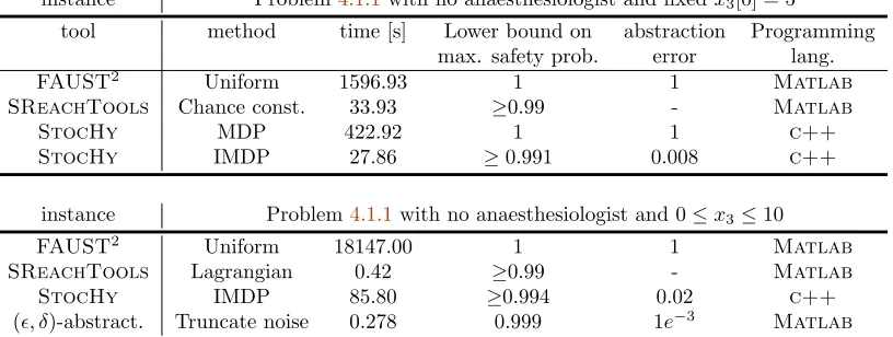
instance Problem4.1.1with no anaesthesiologist and fixedx3[0] = 5
tool method time [s] Lower bound on abstraction Programming max. safety prob. error lang.
FAUST2 Uniform 1596.93 1 1 Matlab
SReachTools Chance const. 33.93 ≥0.99 - Matlab
StocHy MDP 422.92 1 1 c++
StocHy IMDP 27.86 ≥0.991 0.008 c++
instance Problem4.1.1with no anaesthesiologist and 0≤x3≤10
FAUST2 Uniform 18147.00 1 1 Matlab
SReachTools Lagrangian 0.42 ≥0.99 - Matlab
StocHy IMDP 85.80 ≥0.994 0.02 c++
(, δ)-abstract. Truncate noise 0.278 0.999 1e−3
Matlab
Table 8: Results for stochastic viability problem with no anaesthesiologist.
11,??,??, and??. More precisely, each figure depicts the forward reach setsXk (green boxes) starting from the safe set, that is, x0 ∈ X0 =:S for one of the possible input combinations. The blue line gives trajectories starting from the vertices of the safe set. From Figure 11, we observe that most initial states stay in the safe sets, only states in the neighborhood of (x0,1, x0,2, x0,3) = (1,0,0) will leave the safe set atk= 1. Also for inputb(cf. Figure??) most states remain safe except for initial states in the neighborhood of (x0,1, x0,2, x0,3) = (1,0,0). Thus in this neighborhood we observe that the maximal control input is not sufficient to avoid failure if no bolus is applied. This scenario has a low probability.
For input c (cf. Figure ??), most states remain safe except for states in the neighborhood (x0,1, x0,2, x0,3) = (6,10,10) which leave the safe set at k= 1.
In contrast, when the bolus is not given together with the control inputv, the states remain in the safe set. as illustrated for inputdin Figure??.
0 2 4 6 0 5 10 0 5 10 x1 x2 x3 (a) 0 2 4 6 0 5 10 0 5 10 x1 x2 x3 (b) 0 2 4 6 0 5 10 0 5 10 x1 x2 x3 (c)
Figure 13: Forward reach sets for input c are given for k ∈ {0,1} in (a), k∈ {0,1,4} in (b), and fork∈ {0,1,4,10}in (c).
Based on this preliminary analysis, a policy that achieves safety can be composed as
v[k] = (
7, 1≤x1[k]≤3 0, 3< x1[k]≤6.
2 4 6 0 5 10 0 5 10 x1 x2 x3 (a) 2 4 6 0 5 10 0 5 10 x1 x2 x3 (b) 2 4 6 0 5 10 0 5 10 x1 x2 x3 (c)
Figure 14: Forward reach sets for inputd are given for k∈ {0,1} in (a), k∈ {0,1,4} in (b), and fork∈ {0,1,4,10}in (c).
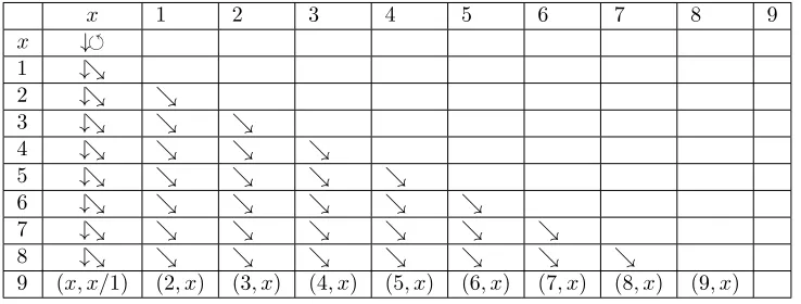
Anaesthesiologist’s actions depends on the past actions and current state The past history of the bolus dosages can be modelled with 46 states and transitions given in Table9.
x 1 2 3 4 5 6 7 8 9
x ↓ 1 ↓& 2 ↓& &
3 ↓& & &
4 ↓& & & &
5 ↓& & & & &
6 ↓& & & & & &
7 ↓& & & & & & &
8 ↓& & & & & & & &
9 (x, x/1) (2, x) (3, x) (4, x) (5, x) (6, x) (7, x) (8, x) (9, x)
Table 9: Bolus counter
4.1.3 Stochastic viability with anaesthesiologist and uncertainty - preliminary analysis
The analysis as discussed in the previous subsection can be extended by adding the noise signalw[k] to the system. Due to the small noise signal, gridding might not be necessary. This conclusion is drawn based on the same reasoning and computations as described in SectionB.0.1. Therefore, the noise is truncated, where the error, denoted withδ, is chosen equal toδ= 0.0001. This yields the Gaussian realizationsw1, w2, w3 to be limited tow1 ∈[−0.1312,0.1312], w2 ∈ [−0.1312,0.1312], w3∈[−0.1312,0.1312]. The new abstract model ˜M with truncated noise, is approximately bisimilar to the original modelM. This is denoted as ˜M ≡=0
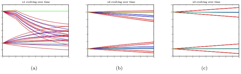
with our automated input is to supply no additional input. On the other hand, if statex1 is high 1≤ x1 ≤3, the worst case scenario is the anaesthesiologist doing nothing at all. Even tough this has a very low probability, it could happen. This could imply that we leave the safe set by exceeding the lower-bound on x1. The best thing we can do with our automated input is to supply as much as possible. This yields the same control strategy as given in (4). The results are given in Figure15. The green lines denote the upper- and lowerbound of the safe set, the red lines are the extrema of the noise and the blue lines the nominal trajectory. The trajectories are shown for all extreme initial conditions inside the safe set. Besides that, the anaesthesiologist has been implemented as described by the worst case scenarios before. The states are not always safe and due to the coupling between the states, it is not possible to conclude anything about the initial set from which this input will guarantee that the original system will always be in the safe set (with a probability of (1−δ)10 = 0.999). The analysis shows that it is necessary to have more advanced tools to solve this problem.
0 1 2 3 4 5 6 7 8 9 10 −1 0 1 2 3 4 5 6 7
x1 evolving over time
(a)
0 1 2 3 4 5 6 7 8 9 10 −2 0 2 4 6 8 10 12
x2 evolving over time
(b)
0 1 2 3 4 5 6 7 8 9 10 −2 0 2 4 6 8 10 12
x3 evolving over time
(c)
Figure 15: Evolution of the state over time,x1in (a),x2in (b),x3 in (c)
4.2
Building Automation System
The Building Automation System (BAS) benchmark is split into three different versions built upon the library of stochastic models presented in [11, 1]. For each model instance (i) we establish the dynamics of the models, (ii) the specification of interest, and (iii) we describe the results of the friendly competition.
4.2.1 CS1BAS
Model This model is a two zone thermal model consisting of a single discrete location and four continuous variables which evolve according to a stochastic difference equation which takes the form of Ms:
x[k+ 1] =Ax[k] +Bu[k] +Q+ ΣW[k]
ys[k] = "
1 0 0 0
0 1 0 0
#
x[k], (5)
with a uniform sampling time ∆ = 15 minutes. Here,
A=
0.6682 0 0.02632 0
0 0.6830 0 0.02096
1.0005 0 −0.000499 0
0 0.8004 0 0.1996
, B=
0.1320 0.1402 0 0
, Q=
3.3378 2.9272 13.0207 10.4166 ,Σ =
0.0774 0 0 0
0 0.0774 0 0
0 0 0.3872 0
0 0 0 0.3098
and W =
w1 w2 w3 w4 T
are independent Gaussian random variables, which are also independent of the initial condition of the process (cf. Section 2.2.1 in [1]).
Specification The thermal model is performing within the comfort range if the temperature in each zone is kept within the range [19.5 20.5] , when using a control input signal which lies within the range of [15 22], for a specific time horizon.
Problem 4.2.1. DefineS1= [19.5 20.5]×[19.5 20.5]. Characterize the set of initial states and an admissible controller such that the probability of the corresponding traces (ys[·]) generated byMs remain withinS for 1.5 hours (i.e. 6 time steps), with a minimum likelihood of0.8.
4.2.2 CS2BAS
Model The second case studies a model similar to Eq. (5) in Section 4.2.1, but as a higher dimensional problem for more model fidelity. In this case, the model is a discrete-time Gaussian-perturbed stochastic linear system with 7-dimensional state, 1-dimensional control input, and a 6-dimensional Gaussian disturbance vector. The traceys[·] in this case is defined as the first component of the state. The model details can be found in [1].
Specification We would like to synthesise a policy ensuring that the temperature within zone 1 does not deviate from the set point by more then 0.5oC over a time horizon equal to 1.5 hours.
Problem 4.2.2. DefineS2= [19.5 20.5]. Characterize the set of initial states and an admissible controller such that the probability of the corresponding traces (ys[·]) generated by Ms remain withinS for 1.5 hours (i.e. 6 time steps), with a minimum likelihood of0.8.
Model manipulationsUsing a singular value decomposition, the rank deficient Bw ∈R7×6 matrix is replaced by an equivalent matrixBw∈R7×4. More specifically,Bw=UΣV0 can be replaced by the equivalent ˜Bw=UΣ.
4.2.3 Results
Problems4.2.1and4.2.2are stochastic viability problems with Gaussian-perturbed linear sys-tem and convex safe set.
SReachTools Since SReachTools analyzes safety under full state information, we use the safe setsS1×R2 andS2×R6 respectively. See Section4.1.1for details of the approaches used in SReachTools. For Problem 4.2.2, SReachTools declares all initial states whose first component lie inS2 can be driven to achieve a safety probability of 0.8.
StocHy synthesises the optimal policy by performing abstractions into an imdp. For this method, we discretise the action space once again resulting in a discrete-time switched system. Note that StocHycould also have solved this problem using the mdpmethod, however due to the length of time needed to generate the abstractions for small abstraction errors this was left out of the comparison for this benchmark.
FAUST2 performs policy synthesis by performing abstractions into
mdp. Both the con-tinuous and action space are discretised depending on the input maximum required level of abstraction, representative points are selected and anmdpis built. The abstract model error increases linearly with the time horizon, hence for longer time horizons one needs to discretise more finely in order to obtain models with smaller abstraction errors.
Figure 16: Stochastic viability set for Problem 4.2.1 for x3[0] = x4[0] = 20, computed using SReachTools. Code available in https://doi.org/10.24433/CO.8093142.v1.
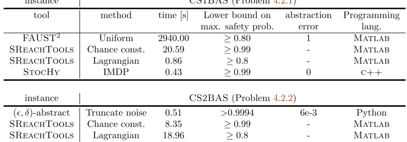
instance CS1BAS(Problem4.2.1)
tool method time [s] Lower bound on abstraction Programming max. safety prob. error lang.
FAUST2 Uniform 2940.00 ≥0.80 1 Matlab
SReachTools Chance const. 20.59 ≥0.99 - Matlab
SReachTools Lagrangian 0.86 ≥0.8 - Matlab
StocHy IMDP 0.43 ≥0.99 0 c++
instance CS2BAS(Problem4.2.2)
(, δ)-abstract Truncate noise 0.51 >0.9994 6e-3 Python
SReachTools Chance const. 8.35 ≥0.99 - Matlab
SReachTools Lagrangian 18.96 ≥0.8 - Matlab
Table 10: Results for stochastic viability analysis for building automation systems. SReach-Toolsdoes not use any abstraction, and analyzes the continuous-state problem directly.
model, or an LTI model with bounded disturbance. For the Building Automation System, only the 7 dimensional model was solved via this approach. For this model it was computed that truncating the noise of the LTI model would be more effective than computing an MDP model. System dynamics are loaded in Python based on the .mat file generated by Matlab in the other benchmarks. The Gaussian disturbance on this model is very low. An estimated amount of 17×109 would be needed to achieve an MDP that has similar performance and which does not have deterministic dynamics. In Table10, the computation time is given together with the probability that the system starting from a stationary state leaves the safe set.
4.3
Heated Tank
4.3.1 Description
The Heated Tank benchmark stems from safety literature; there it is a well-known example of a Piecewise Deterministic Markov Process (PDMP) [16]. This made the Heated Tank benchmark a logical candidate for early inclusion in the set of ARCH stochastic models [1].
The heated tank system consists of a tank containing liquid whose level is influenced by two pumps and one valve managed by a controller. The purpose of the liquid in the tank is to absorb and transport the heat from a heat source; this means that under nominal conditions one of the pumps produces a constant inflow of cool liquid, and a similar flow of heated liquid leaves the tank through the valve. The Euclidean valued state components are the heightxH,t and temperaturexT ,t of the liquid in the tank at momentt. Pumps and Valve may fail, and a Controller switches Pumps or Valve if the height of the liquid becomes too high or too low. The rare event probabilities, to be estimated on time interval [t0, tend], are: Dryout probability (pdryout), Overflow probability (poverf low), and Overheating probability (poverheating). The heated tank benchmark has five versions:
- Version 1: Pumps and Valve have constant failure rates;
- Version 2: Pumps and Valve have mode dependent failure rates;
- Version 3: In version 1, Controller may fail to implement its switching decision;
- Version 4: In version 1, Pumps and Valve are repaired;
- Version 5: In version 1, failure rates depend on the liquid temperature.
For ARCH2018 the focus has been on the estimation of the dryout probability for version 4 [1] using the methods Modest Toolset and SDCPN & Monte Carlo simulation. The very reason for this focus was that it is a rare event estimation type of problem.
4.3.2 ARCH2019 objectives
For ARCH2019 one objective is to apply two novel methods to version 4 of the heated tank benchmark: HYPEGandSDCPN&IPS. A complementary objective is to make the heated tank benchmark more challenging by extending version 4 with other complications, e.g. from versions 2, 3 or 5. In order to specify such extensions in an unambiguous way it is needed to move from a textual type of heated tank benchmark description to a formal model description.
4.3.3 ARCH2019 results
A. Rare event estimation results
For the heated tank version 4, Table11lists the parameter values that have been used in the estimation of the dry-out probability.
Parameter Symbol values in version 4 Failure rate of P1 λP1 2.2831×10⁻³ h−1 Failure rate of P2 λP2 2.8571×10⁻³ h−1 Failure rate of V λV 1.5625×10⁻³ h−1
Repair rate µ 0.2h−1
Liquid flow q 0.6m/h
Normalized input energy Ein 1oCm/h Luiqid inflow temperature Tin 15oC
Initial liquid temperature Tinit 152/3oC Liquid overflow level HOverf low 5 m
Liquid too high level HHigh 1 m
Liquid initial level Hinit 0 m
Liquid too low level HLow -1m
Liquid dryout level HDryout -5m
Initial time t0 0h
End time tend 500h
Table 11: Parameters and their values in version 4
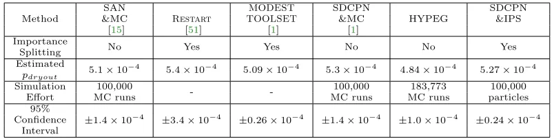
Table12gives thepdryoutestimation results obtained by the different methods; i.e. SAN&MC, Restart,Modest Toolset,SDCPN&MC,HYPEGandSDCPN&IPSrespectively. Of these methods,Restart,Modest ToolsetandIPShave in common of using splitting tech-niques in MC simulation of rare events. The importance functions that are used byRestart andModest Toolsetcounts the number of component failures that are relevant for dry-out. The importance function that is used by IPS is the distance between liquid height xH,t and
HDryout.
Method
SAN MODEST SDCPN SDCPN
&MC Restart TOOLSET &MC HYPEG &IPS [15] [51] [1] [1]
Importance No Yes Yes No No Yes
Splitting Estimated
5.1×10⁻⁴ 5.4×10⁻⁴ 5.09×10⁻⁴ 5.3×10⁻⁴ 4.84×10⁻⁴ 5.27×10⁻⁴ pdryout
Simulation 100,000
- - 100,000 183,773 100,000
Effort MC runs MC runs MC runs particles
95%
±1.4×10⁻⁴ ±3.4×10⁻⁴ ±0.26×10⁻⁴ ±1.4×10⁻⁴ ±1.0×10⁻⁴ ±0.24×10⁻⁴
Confidence Interval
Table 12: pdryout estimation results: two from safety literature (SAN & MC andRestart), two from methods applied in ARC2018 (Modest Toolset and SDCPN & MC), and two from the new methodsHYPEGandSDCPN&IPS.
For the readers that are not familar withModest Toolset, we refer to [30]. We used the hierarchical description formalisms shown below for version 4.
const realtend; const realHOverf low; const realHHigh; const realHLow; const realHDryout; const realλP1; const realλP2; const realλV; const realµ;
const realCf ail= 0; action init;
bool on p1 = true, on p2 = false, on v = true; int(0..2) fail p1, fail p2, fail v;
varxH,t= 0;
der(xH,t) = (on p1 && fail p1 == 0k fail p1 == 1 ? 0.6 : 0) + (on p2 && fail p2 == 0 k fail p2 == 1 ? 0.6 : 0) + (on v && fail v == 0k fail v == 1 ? -0.6 : 0);
bool overflow, dryout; int(0..2) grace;
propertypdryout = Pmax(<>[T<=tend] dryout);
property IDryOut = (fail p1 == 2 ? 1 : 0) + (fail p2 == 2 ? 1 : 0) + (fail v == 1 ? 1 : 0);
process Pump1() {
clock c; real x;
invariant(false) init {= x = Exp(λP1) =}; do{
when(c>= x) invariant(c<= x) palt{ :1:{= fail p1 = 1 =}
:1:{= fail p1 = 2 =} };
when(grace ! = 0) invariant(grace == 0){= c = 0, x = Exp(µ) =}; alt{
:: when(c>= x) invariant(c<= x){= fail p1 = 0, c = 0, x = Exp(λP1) =} :: when(grace == 2) invariant(grace ! = 2) break
} } }
process Pump2() {
clock c; real x;
invariant(false) init {= x = Exp(λP2) =}; do{
:1:{= fail p2 = 2 =} };
when(grace ! = 0) invariant(grace == 0){= c = 0, x = Exp(µ) =}; alt{
:: when(c>= x) invariant(c<= x){= fail p2 = 0, c = 0, x = Exp(λP2) =} :: when(grace == 2) invariant(grace != 2) break
} } }
process Valve() {
clock c; real x;
invariant(false) init {= x = Exp(λV) =}; do{
when(c>= x) invariant(c<= x) palt{ :1:{= fail v = 1 =}
:1:{= fail v = 2 =} };
when(grace ! = 0) invariant(grace == 0) = c = 0, x = Exp(µ) =; alt{
:: when(c>= x) invariant(c<= x) = fail v = 0, c = 0, x = Exp(λV) = :: when(grace == 2) invariant(grace != 2) break
} } }
process Controller() {
process Normal() {
alt{
:: invariant(level<=HHigh) when(level>=HHigh) palt{
:1−Cf ail:{= on p1 = false, on p2 = false, on v = true, grace = 1 =} :Cf ail:{= grace = 1 =}
}; High()
:: invariant(level>=HLow) when(level<=HLow) palt{
: 1−Cf ail:{= on p1 = true, on p2 = true, on v = false, grace = 1 =} : Cf ail: {= grace = 1 =}
}; Low() }
}
process High() {
invariant(level>=HLow) when(level<=HLow) palt{ : 1−Cf ail :{= on p1 = true, on p2 = true, on v = false =} :Cf ail:{==}
process Low() {
invariant(level<=HHigh) when(level>=HHigh) palt{ : 1−Cf ail :{= on p1 = false, on p2 = false, on v = true =} : Cf ail: {==}
}; High() }
Normal() }
process Observer() {
par{
:: invariant(level<=HOverf low) when(level>=HOverf low){= overflow = true, grace = 2 =}
:: invariant(level>=HDryout) when(level<=HDryout){= dryout = true, grace = 2 =}
} } par{ :: Pump1() :: Pump2() :: Valve() :: Controller() :: Observer() }
C. HPnG model of heated tank benchmark version 4
SinceHYPEG is a simulator for hybrid Petri nets with general transitions (HPnGs) [27], the heated tank benchmark has been modeled as an HPnG. A graphical representation of the HPnG for version 4 of the heated tank benchmark is presented in Figures18 to21, divided into four parts, which compose one large HPnG (connected via places with identical names in different figures).
Figure 17: Graphical representation of HPnG components [37].
Figure 18shows how the state of the valve is modeled via four different discrete places V On,
V Off, V SOn, V SOff. The token (small black circle) can be transported to another discrete place, thus switching the valve state via general transitions, e.g. V On SOn, or immediate transi-tions, e.g. V On Off. The firing times of the general transitions for the valve follow exponential distributions with rateλV. The immediate transitions can only fire when there is a token in the places Increaseor Decrease, due to the connecting test arcs. The state of the valve is further stored in the places Valve On and Valve Off, which is required for the filling of the tank (see Figure20). When the valve is in stuck mode, the repair is modeled by the general transitionsV SOff Repairresp. V SOn Repair, which are enabled when the placeValve grace
holds a token and follow an exponential distribution with repair rateµ.
Figure 18: HPnG of the heated tank version 4: Valve.
Figure 19: HPnG of the heated tank version 4: Pumps.
Figure20shows how the heated tank and its controller are modeled. The fluid level of the heated tank is modeled by the continuous placex H, which has two static continuous input transitions
H in1andH in2, with a rate ofqresp. 2·q, and one static continuous output transitionH out
with rateq. The transitions get enabled via test arcs or inhibitor arcs, depending on the number of tokens in the placesOne PumpandTwo Pumps andValve On.
The controller is initially in theNormalstate, but moves toIncreaseor Decrease, when the transitionNormal Decreaseresp. Normal Increasefires. SinceNormal Decreaseis controlled by a test arc, it gets enabled when the fluid level of x Hreaches the weight of the test arc, i.e.
HHigh. On the other hand, Normal Increase is controlled by an inhibitor arc and thus gets enabled whenx H < HLow. In a similar way, the token can further move between Increase andDecrease via the transitions Decrease Increaseand Increase Decrease. The firing of
Normal Increase resp. Normal Decrease further adds a token into the places Valve grace,
P1 graceandP2 grace, activating the repair mode for the components. Each of these places can lose its token via the connected immediate transitions for the case of an outflow or dryout, i.e. when the fluid level ofx H reachesHDryout orHOverf low.
Figure 20: HPnG of the heated tank version 4: Tank and Controller.
D. SDCPN model of heated tank benchmark version 4
The graphical part of theSDCPNmodel is given in Figure22; it has one local Petri Net (LPN) for each of the systems Pump 1(P1), Pump 2(P2), Valve(V), Tank(T), and Controller(C). Figure 22shows the places, the transitions 2 and the arcs (→or –•) within and between each of these fiveLPN’s. Figure22 also shows which places have a token at initial momentt0. Each LPNis such that it always has exactly one token.
For readers that are not familiar withSDCPN, we provide a short explanation of the graphical elements in thisSDCPNmodel. Arcs ending with an arrow are normal arcs; arcs ending with a ball are enabling arcs. In contrast with a normal arc, an enabling arc can only go from a place to a transition, and this transition does not consume any token from this place. Each enabling arc that starts from the boundary of a local Petri net (LPN) and ends at the boundary of another local Petri net (LPN), say fromLPN A toLPNB, represents multiple enabling arcs, i.e. one enabling arc for each combination of a place inLPNA and a transition inLPNB. This allows that all transitions inLPN B have full access to the hybrid state information available in LPN A. There are three types of transitions: Immediate transitions (I), Delay transitions (D) and Guard transitions (G). A transition is said to be pre-enabled if each place from which it receives an arc has a token. If an immediate transition is pre-enabled it fires a token to the places where outgoing arcs lead to. If a delay transition is pre-enabled then its firing happens stochastically at a given firing rate. If a guard transition is pre-enabled, then it fires as soon as its guard condition is satisfied.
If in LPN “Tank” there is a token in place Normal, i.e θT ,t = N ormal, then to this token a 2-D Euclidean valued process {xH,t, xT ,t} is connected which is the solution of the following differential equations:
dxH,t=q·(χP1,t+χP2,t−χV,t)·dt withxH,0=Hinit
dxT ,t=[q·(χP1,t+χP2,t)(Tin−xT ,t) +Ein]/(xH,t−HDryout)·dt withxT ,0=Tinit
where forU ∈ {P1, P2, V}:χU,t = 1 if LPNU has a token in place Onor in place StuckOn, elseχU,t= 0.
InLPN “Tank” the guard conditions of G1 and G2 arexH,t≥HOverf low andxH,t≤HDryout respectively.
InLPN “Controller” the guard conditions of G1, G2, G3 and G4 arexH,t ≥HHigh, xH,t ≤
HLow,xH,t≤HLowand xH,t≥HHigh respectively.
InLPN’s Pump 1, Pump 2 and Valve the following applies to the transitions:
– Di, i∈ {1,2,3,4} fires at rateλU,U ∈ {P1, P2, V}. – Di, i ∈ {5,6,7,8} fires at rate 1
2µ6= 0 , iff the token of LPN Controller is not in place
N ormal.
– In LPN Pj, j=1,2, I1 fires if Pj's place Of f has a token as well as LPN C's place
Increase,
– InLPNV, I1 fires if V's placeOf f has a token as well asLPN C's place Decrease, – InLPNPj, j=1,2, I2 fires ifPj's placeOnhas a token as well asLPNC's placeDecrease, – InLPNV, I2 fires if V's placeOnhas a token as well asLPNC's placeIncrease.
The Generalised Stochastic Hybrid Process (GSHP) defined by thisSDCPNmodel is{xt, θt} with xt = [xH,t, xT ,t]T and θt = [θU,t;U =P1, P2, V, T, C]T , where the value of processθU,t equals the name of the place where the token inLPNU is at momentt.
E. Relevant extensions of heated tank benchmark
I. Discrete-valued process influences repair rates or failure rates (e.g. in version 2).
II. Non-zero probability of not communicating a decision made (e.g. in version 3)
III. Continuous-valued process influences repair rate or failure rate (e.g. in version 5).
IV. Non-exponentially distributed duration of working and/or repair of system components.
V. Brownian motion in a Euclidean state component, e.g. in the heat source Ein.
For the modelling of these extensions it also is quite helpful if the syntax supports compositional modelling. In Table13, it is indicated which extensions are supported by PDMP, by GSHP and by which of the three syntax models that have been used for the Heated tank benchmark, i.e. Modest Toolset,SDCPNand HPnG.
Model syntax I II III IV V Compositional modelling
PDMP Yes Yes Yes Yes No No
GSHP Yes Yes Yes Yes Yes No
Modest Toolset Yes Yes No Yes No Yes
HPnG Yes Yes No Yes No Yes
SDCPN Yes Yes Yes Yes Yes Yes
Table 13: Capabilities of the methods to support relevant extensions.
4.4
Tandem Network
4.4.1 Model
Let us first give solution to the time bounded reachability problem overctmcs in general and then we will discusstandem network as a concrete example.
A continuous-time Markov chain (ctmc) M = (SM, R) consists of a finite set SM = {1,2,· · · ,|SM|}of states, a rate matrixSM×SM →R≥0. Intuitively, R(s, s0)>0 indicates that a transition fromstos0 is possible and that the timing of the transition is exponentially distributed with rateR(s, s0). Q is the infinitesimal generator matrix of M defined as Q =
R−diags(Ps0∈SMR(s, s0)). Note that P
s0Q(s, s0) = 0 for any s ∈ SM. Let M = (S] {good,bad}, R) be actmc, with|S|=m, and absorbing statesgoodandbad. For computing the reachability probability vectorZ(t) we need to solve for the following differential equation
d
dtZ(t) =QZ(t), Z(0) =1(good), (6)
where Z(t) ∈ Rm is a column vector with elements Zi(t) = ProbM(1(si), t), denoting the probability of reaching thegood state after timet for theith state and 1(i) denotes a m×1 vector which contains zeros everywhere and 1 on itsithposition. In order to solve Equation (6) the most common approach is to use uniformization. By using uniformization, one can compute time bounded reachability for an arbitrary time bound with an arbitrary precision. However, it is well-known that for large time bounds, uniformization is not fast enough.
Time bound [h] run-time [s] reach. prob
333.34 0.019 0.153
666.67 0.011 0.284
1000 0.012 0.394
1333.34 0.012 0.487
1666.67 0.015 0.566
Table 14: Results for runningLyapMMCovertandem network usingε(T)=0.01
Formal error bound (ε(T)) [h] run-time [s] Percentage of order reduction
0.5 0.0056 25.2%
0.4 0.008 16.5%
0.3 0.009 9.56%
0.2 0.01 3.4%
0.1 0.018 0%
Table 15: Results for runningLyapMMCovertandem network with differentε(T)
the computation pespective, instead of (6), a set of differential equations of orderr(r << m) will be solved,
d dt
¯
Z(t) = ¯QZ¯(t), Z¯(0) = ¯Z0, (7)
where ¯Z(t)∈Rr×1and ¯Q, ¯Z0 should be computed such that
Z(t)−PZ¯(t)
≤ε(t), (8)
whereP∈Rn×ris a projection matrix andεdenotes the time varying upper bound over order reduction error. The details on the computation of ¯Q,Z¯0 and P and the characterization of
ε(t) can be found in [40].
We consider cap = 10 which results in a ctmc with 231 states. We can choose values
µ1 = 1, µ2 = 2, κ = 2, λ = 4, a = 1, b = 0 and time bounds T = 60000×r for r being integers from 1 to 5. Once the tandem network is modelled as actmc, the generator matrix
Qis computed such thatblock state (chosen as thegood(absorbing) state) is made absorbing. All we need to do is to compute ¯Q,Z¯0, P forε(t) and solve (7) up-to timeT.
4.4.2 Results
5
Discussion
A highlight of this year’s edition has been the evident and ever growing interest in tools that can verify and perform synthesis of stochastic models. We have seen the introduction of three new software tools and of one early synthesis framework, which together can tackle different problems and benchmarks. Building on the experience gathered from the outcomes of the friendly competition and from the work on the benchmarks (old and new), some key points for future work have been identified as follows:
• one of the key issues is the absence of an accepted formal modelling description for the benchmarks, which would (among other things) facilitate their comparison and the run-ning of experiments on them. It is understood that there is a plethora of stochastic models characterisations, each of which are tailored to specific tasks and problems (e.g., rare-event setup, or a control setup), however there is a need for a common modelling language. Related to this is also the need for a common format for sharing models used in the benchmarks (e.g. .matfiles);
• many tools have different ways to describe outcomes, which are tailored towards the underlying of algorithms used within specific tools. A common standard for the output of tools is required (e.g., max satisfiability for a specific initial condition);
• it was noted that in most of the current benchmarks the effect of noise is small, hence we should design models where noise has a larger effect on the dynamics;
• a realistic safety analysis problem of industrial relevance is typically is much larger than what can be currently handled in an ARCH benchmark;
• there is a need for more diverse specifications, beyond safety or reach-avoid;
• finally, we should work towards having all tools working on benchmarks run over the same machine.
6
Conclusion
This report has presented the results of a first friendly competition for the formal verification of stochastic models, as part of the ARCH’19 Workshop. The reports of other categories can be found in the proceedings and on the ARCH website: cps-vo.org/group/ARCH.
7
Acknowledgments
This work is partially supported by the Alan Turing Institute, UK and Malta’s ENDEAVOUR Scholarships Scheme. We thank Dr. Mariken Everdij (NLR) for syntax verification of the SDCPNmodel specification for the heated tank version 4.
References
[2] Alessandro Abate, Maria Prandini, John Lygeros, and Shankar Sastry. Probabilistic reachability and safety for controlled discrete time stochastic hybrid systems. Automatica, 44(11):2724–2734, 2008.
[3] A Absalom and G Kenny. ‘paedfusor’ pharmacokinetic data set. British Journal of Anaesthesia, 95(1):110–110, 2005.
[4] H.A.P. Blom, J. Krystul, G.J. Bakker, M.B. Klompstra, and B. Klein Obbink. Free flight collision risk estimation by sequential Monte Carlo simulation. In C.G. Cassandras and J. Lygeros, editors, Stochastic Hybrid Systems, pages 249–281. Taylor & Francis/CRC Press, 2007.
[5] H.A.P. Blom, H. Ma, and G.J. Bakker. Interacting Particle System-based Estimation of Reach Probability for a Generalized Stochastic Hybrid System. InIFAC Conference on Analysis and Design of Hybrid Systems, pages 79–84, Oxford, UK, 2018.
[6] Olivier Bouissou, Eric Goubault, Sylvie Putot, Aleksandar Chakarov, and Sriram Sankara-narayanan. Uncertainty propagation using probabilistic affine forms and concentration of measure inequalities. InInternational Conference on Tools and Algorithms for the Construction and Anal-ysis of Systems, pages 225–243. Springer, 2016.
[7] Carlos E. Budde, Pedro R. D’Argenio, and Arnd Hartmanns. Better automated importance split-ting for transient rare events. InThird International Symposium on Dependable Software Engi-neering. Theories, Tools, and Applications (SETTA), volume 10606 ofLecture Notes in Computer Science, pages 42–58. Springer, 2017.
[8] Carlos E. Budde, Pedro R. D’Argenio, Arnd Hartmanns, and Sean Sedwards. A statistical model checker for nondeterminism and rare events. In24th International Conference on Tools and Algo-rithms for the Construction and Analysis of Systems (TACAS), volume 10806 ofLecture Notes in Computer Science, pages 340–358. Springer, 2018.
[9] Carlos E Budde, Christian Dehnert, Ernst Moritz Hahn, Arnd Hartmanns, Sebastian Junges, and Andrea Turrini. Jani: Quantitative model and tool interaction. InInternational Conference on Tools and Algorithms for the Construction and Analysis of Systems, pages 151–168. Springer, 2017. [10] Manuela L Bujorianu and John Lygeros. Toward a general theory of stochastic hybrid systems.
InStochastic hybrid systems, pages 3–30. Springer, 2006.
[11] Nathalie Cauchi and Alessandro Abate. Benchmarks for cyber-physical systems: A modular model library for buildings automation. InIFAC Conference on Analysis and Design of Hybrid Systems, 2018.
[12] Nathalie Cauchi and Alessandro Abate. StocHy: automated verification and synthesis of stochastic processes. In 25th International Conference on Tools and Algorithms for the Construction and Analysis of Systems (TACAS), 2019.
[13] Nathalie Cauchi, Luca Laurenti, Morteza Lahijanian, Alessandro Abate, Marta Kwiatkowska, and Luca Cardelli. Efficiency through uncertainty: Scalable formal synthesis for stochastic hybrid systems. In22nd ACM International Conference on Hybrid Systems: Computation and Control (HSCC), 2019. arXiv: 1901.01576.
[14] Fr´ed´eric C´erou, Pierre Del Moral, Fran¸cois Le Gland, and Pascal Lezaud. Genetic genealogical models in rare event analysis. ALEA, Latin American Journal of Probability and Mathematical Statistics, 1:181–203, 2006.
[15] D. Codetta-Raiteri. Modelling and simulating a benchmark on dynamic reliability as a stochastic activity network. In23rd European Modeling and Simulation Symposium (EMSS), pages 545–554, 2011.
[16] M.H.A. Davis. Markov models and optimization, volume 49. Chapman and Hall/CRC, 1993. [17] Christian Dehnert, Sebastian Junges, Joost-Pieter Katoen, and Matthias Volk. A storm is coming:
A modern probabilistic model checker. InInternational Conference on Computer Aided Verifica-tion, pages 592–600. Springer, 2017.
[19] M.H.C. Everdij and H.A.P. Blom. Bisimulation Relations Between Automata, Stochastic Differ-ential Equations and Petri Nets. In M. Bujorianu and M. Fisher, editors,Electronic Proceedings in Theoretical Computer Science, volume 20, pages 1–15. 2010.
[20] M.H.C. Everdij and H.A.P. Blom. Hybrid state petri nets which have the analysis power of stochastic hybrid systems and the formal verification power of automata. In P. Pawlewski, editor, Petri Nets, pages 227–252. I-Tech Education and Publishing, 2010.
[21] M.H.C. Everdij, Margriet B. Klompstra, H.A.P. Blom, and Bart Klein Obbink. Compositional Specification of a Multi-agent System by Stochastically and Dynamically Coloured Petri Nets. In H.A.P. Blom and J. Lygeros, editors, Stochastic Hybrid Systems: Theory and safety critical applications, pages 325–350. Springer, 2006.
[22] Victor Gan, Guy A Dumont, and Ian Mitchell. Benchmark problem: A pk/pd model and safety constraints for anesthesia delivery. InARCH@ CPSWeek, pages 1–8, 2014.
[23] Hamed Ghasemieh, Anne Remke, and Boudewijn R. Haverkort. Survivability evaluation of fluid critical infrastructures using hybrid Petri nets. In19th IEEE Pacific Rim International Symposium on Dependable Computing, pages 1–10. IEEE CS Press, 2013.
[24] Hamed Ghasemieh, Anne Remke, and Boudewijn R. Haverkort. Survivability analysis of a sewage treatment facility using hybrid Petri nets. InPerformance Evaluation, pages 1–21. Elsevier, 2015. [25] Joseph D. Gleason, Abraham P. Vinod, and Meeko M. K. Oishi. Underapproximation of reach-avoid sets for discrete-time stochastic systems via lagrangian methods. InIEEE Conference on Decision and Control (CDC), pages 4283–4290, Dec 2017.
[26] J. Greifeneder and G. Frey. Probabilistic hybrid automata with variable step width applied to the analysis of networked automation systems. InProc. 3rd IFAC Workshop on Discrete Event System Design (DESDes’06), pages 283–288. IFAC, September 2006.
[27] Marco Gribaudo and Anne Remke. Hybrid Petri nets with general one-shot transitions. Perfor-mance Evaluation, 105:22–50, 2016.
[28] Sofie Haesaert, Nathalie Cauchi, and Alessandro Abate. Certified policy synthesis for general markov decision processes: An application in building automation systems. Performance Evalua-tion, 117:75–103, 2017.
[29] Sofie Haesaert, Sadegh Esmaeil Zadeh Soudjani, and Alessandro Abate. Verification of general Markov decision processes by approximate similarity relations and policy refinement.SIAM Jour-nal on Control and Optimization, 55(4):2333–2367, 2017.
[30] E. M. Hahn, A. Hartmanns, H. Hermanns, and J.P. Katoen. A compositional modelling and analysis framework for stochastic hybrid systems. Formal Methods in System Design, 43(2):191– 232, 2013.
[31] Ernst Moritz Hahn, Arnd Hartmanns, Holger Hermanns, and Joost-Pieter Katoen. A composi-tional modelling and analysis framework for stochastic hybrid systems.Formal Methods in System Design, 43(2):191–232, 2013.
[32] Arnd Hartmanns and Holger Hermanns. The Modest Toolset: An integrated environment for quantitative modelling and verification. In20th International Conference on Tools and Algorithms for the Construction and Analysis of Systems (TACAS), volume 8413 ofLecture Notes in Computer Science, pages 593–598. Springer, 2014.
[33] M. Herceg, M. Kvasnica, C.N. Jones, and M. Morari. Multi-Parametric Toolbox 3.0. InProc. of the European Control Conference, pages 502–510, Z¨urich, Switzerland, July 17–19 2013. http: //control.ee.ethz.ch/~mpt.
[34] H. Hermanns. Multi terminal binary decision diagrams to represent and analyse continuous time Markov chains, pages 188–207. 1999.

![Figure 9: The lower probability of satisfying safety property when xare given in Tableis generated using3[0] = 5 is fixed and policy StocHy via abstractions into imdp](https://thumb-us.123doks.com/thumbv2/123dok_us/8876372.1817106/14.612.224.391.316.446/figure-probability-satisfying-property-tableis-generated-stochy-abstractions.webp)