Testing for Multiple Bubbles in Asset Prices
Nikolaus Landgraf
∗Abstract
Detecting the presence of bubbles in asset prices has become a major interest for policy makers and central banks. By an early identification of a bubble it might be possible for them to intervene and prevent the asset price from collapsing. For this purpose, several econometric tests were invented and some of which summarized by Homm and Breitung (2011). The power of one of the statistics, the sup augmented Dickey- Fuller (SADF) statistic, was improved by Phillips, Shi and Yu (2012). They developed a new recursive strategy and proposed the general SADF statistic.
The present thesis approaches the sup Bhargava and the sup DFC statistic similarly and computes the power of all statistics on five different bubble generating processes using Monte Carlo Simulations. It turned out that the modified DFC statistic and the general SADF statistic have highest rejection frequencies on processes that generate multiple bub-bles, while the simple sup DFC statistic performed best on processes that do not burst. Application was conducted to the internet currency Bitcoin and the Japanese stock Index Nikkei 225. In both instances, the findings of the power investigation were confirmed. Since both series include bursting bubbles, the simple sup Bhargava and sup DFC statistics were not able to detect a bubble. On the other hand, the modified sup DFC and the general SADF statistics showed clear evidence in favor of the presence of a bubble in both series.
∗
Nikolaus Landgraf received a bachelor degree in Econometrics & Operations Research at Maastricht Univer-sity in 2015. He currently pursues a Master in Quantitative Finance at Erasmus UniverUniver-sity Rotterdam
1 Introduction
Whether it was greed, low interest rates, speculation or just irrational exuberance, economic and financial bubbles have evolved and collapsed throughout history again and again. One of its first kind was the famous Tulipomania. In the 1630s, a bulb in Amsterdam might easily be sold for an annual income of a wealthy merchant (Dash, 2001). A more recent example that still impacts global economy is the United States housing bubble of 2006- 2008. Low interest rates in the United States of America have contributed to extremely rising house prices and therefore to a surge in its price index, the Case-Shiller home price index. In 2008, this index reported its largest drop in history. That was the start of the following credit crisis, which is considered to be the primary cause of the recession in the United States and henceforth of the global financial crisis (Holt, 2009).
Since the existence of bubbles is far from being a phenomenon nowadays and their bursting have not only affected economies but also destroyed people’s savings (e.g U.S. housing bubble), policy makers and central banks have developed a major interest in detecting and testing for the presence of bubbles. Once a bubble is detected policies can be implemented and the effects of a bubble collapse might be prevented. In order to test for the presence of a bubble one first needs to understand what factors drive the price of an asset. Consider below the standard asset pricing equation (Phillips, Shi andYu (PSY), 2012):
Pt= ∞ X
i=0
³ 1 1+rf
´i
E(Dt+i+Ut+i)+Bt, (1)
where Pt is the price of the asset, Dt is the payoff gained from the asset,Ut denotes the unobservable fundamentals,rf is the risk-free interest rate andBt represents the bubble com-ponent. Furthermore,Ptf =Pt−Bt is the so called market fundamental andBt is supposed to have a submartingale property:
E(Bt+1)=(1+rf)Bt. (2)
null of no bubble on various Data Generating Processes (DGP). PSY (2012) on the other hand, have improved the power of one of the tests summarized by Homm and Breitung by varying the tests’ time interval. Particularly on processes including multiple bubbles with periodically collapsing behavior the new test showed improvements in power.
This served as inspiration for the aim of this thesis. Specifically, the objective is to use a similar trick and vary the time interval of two certain tests, namely the Bhargava statistic and a Chow type unit root statistic named DFC, and compare and investigate their power to the basic statistics as well as the statistic found by PSY (2012). This is done by testing the statistics’ rejection frequencies on different DGPs containing both, single and multiple bubbles.
The thesis is structured as follows: at first, section 2 will introduce the above stated test statistics. Moreover, the variation of the time interval will be explained in detail. In section 3, Monte Carlo Simulations will determine the tests’ critical values. Thereafter, five Bubble Gener-ating Processes are illustrated and used to compute the power of the statistics. In section 4, the tests are applied on real data. As test instances, the internet currency Bitcoin and Japan’s stock Index Nikkei 225 are chosen. Lastly, section 5 will conclude and summarize the findings.
2 Test Statistics
As stated in the Introduction, Homm and Breitung (2011) have provided an overview of possible test statistics in order to test for the presence of bubbles. All tests are grounded on the time-varying autoregressive model of order one:
yt=ρtyt−1+ǫt, (3)
whereǫt is a white noise with zero mean and variance equal toσ2. Furthermore, the initial value of the series isy0=c< ∞. Due to simplification, a constant is omitted. The constant in a
stock price series, however, is insignificant anyways. If the reader might want to account for the missing constant, the series can be detrended at first1. Note that the critical values provided in section 3 will be misspecified then.
Under the null hypothesis, equation (3) is a pure random walk for allt. Hence,
H0: ρt =1 t=1, ...,T. (4)
On the other hand, the alternative hypothesis states that yt starts as a random walk and switches to an explosive process at time [τ∗T] withτ∗∈(0, 1):
H1: ρt= (
1 t=1, ..., [τ∗T]
ρ∗>1 t=[τ∗T]+1, ...,T. (5)
1To detrend run the following OLS regression and use its residuals asy
Contrary to the standard unit root tests, in which it is tested whether|ρ| <1, this is a right-tailed test. In other words,H0is rejected for large statistic values. How to compute these statistic
values is being presented in the following subsections.
2.1 The SADF and GSADF Tests
The sup augmented Dickey-Fuller test (SADF), was introduced by Phillips, Wu and Yu (2011, PWY). In order to obtain the SADF statistic it is necessary to first regress the augmented Dickey-Fuller regression model:
∆yt=αr1,r2+βr1,r2yt−1+ k X
i=1
ψir1,r2∆yt−i+ǫt, (6)
in whichǫtis normally distributed with zero mean and varianceσ2r1,r2andk
2represents the
lag order. The numbersr1andr2indicate the starting and end point of the regression in means
of fractions of the total sample. For instance, assumer1=0.2,r2=0.6 and the sample size is 100.
Then the regression would start at the 20th observation and will include the 60th observation as its last one. The ratio of ˆβand its standard error yields the ADFr2
r1 statistic. By fixingr1=0 and expandingr2fromr03to 1, one gets a series of ADF statistics. The supreme of this series is
the SADF statistic. Mathematically speaking, the SADF statistic is denoted by supr2∈[r0,1]ADFr2
0 .
Since the SADF statistic showed inconsistency in the presence of multiple bubbles, PSY (2012) extended the statistic by additionally varying the starting pointr1from 0 tor2−r0. This
trick implied a broader sample sequence and increased the power of the statistic significantly. PSY called this statistic the General sup augmented Dickey-Fuller (GSADF) statistic. It can be expressed as
GS ADF(r0)= sup
r2∈[r0,1] r1∈[0,r2−r0]
©
ADFr2 r1 ª
. (7)
As outlined in the Introduction, this simple trick of increasing the power of a statistic led to the attempt of applying it on other statistics as well. Therefore, I chose the Bhargava statistic and the DFC statistic to be transformed similarly. How both statistics are computed is explained in the upcoming subsections.
2the lag order k was set to 0 in all computations in this thesis. 3r
2.2 The General Sup Bhargava Statistic
One of the statistics summarized by Homm and Breitung (2011) was the Bhargava statistic. They modified the original statistic in order to be able to test for a change from an I(1) process to an explosive one in the intervalr1∈[0, 1−τ0]:
Br2 r1 =
1 [Tr2]−[r1T]
µ P[Tr2]
t=[r1T]+1(yt−yt−1)
2
P[Tr2]
t=[r1T]+1(yt−y[r1T])
2
¶−1
. (8)
In contrast to the SADF statistic, the sup Bhargava statistic is computed by fixing r2=1
and expanding r1 from 0 to 1−r0. Mathematically, supB =supr1∈[0,1−r0]B
1
r1. The reasoning behind this statistic is that, based on the assumption of a random walk process, the sum of squared forecast errors of this series become very large if the process shows explosive behavior. Meaning, the statistic grows large if a bubble exists and the null of no bubble can be rejected.
Applying the interval varying method to the supB statistics means to loosen the fixedr2and
notr1as in the SADF case. This can be done in a feasible range, leading to a statistic that I call
the General sup Bhargava (GsupB) statistic:
G supB(r0)= sup
r2∈[r0,1] r1∈[0,r2−r0]
©
Br2 r1 ª
. (9)
The different interval methods of the supB and GsupB statistics are illustrated in Figure 1. From the right hand side it becomes clear that the end pointr2moves. This fact enables the
possibility to test the statistic on intervals containing only the explosive growth of a bubble and not its collapse. Hence, time series including bubble collapses or even multiple bubbles can be approached in a way that is in line with the underlying hypotheses described in section 2.1.
2.3 The General Sup DFC Statistic
The second statistic is a Chow-type Dickey-Fuller statistic named DFC. As the name suggests, the idea is to use a Chow test to check for a structural break inρt. Letρt =1 fort=1, ..., [r1T]
andρt−1=δ>0 fort=[r1T]+1, ...,T. Then, the regression model is:
∆yt=δ(yt−11© t>[r1T]
ª)+ǫt, (10)
with1© t>[r1T]
ª being an indicator function, which takes on the value 1 if the expression in
curly braces is true and 0 otherwise. To test for a structural break, one needs to test the null hypothesisH0: δ=0, against the alternativeH1: δ>0. The DFC statistic is nothing else than
Figure 1: Illustration of the supB, supDFC (left) and GsupB, GsupDFC (right) time intervals
DF Cr2 r1 =
P[Tr2]
t=[r1T]+1∆ytyt−1 ˜
σqP[Tr2] t=[r1T]+1y
2
t−1
, (11)
where ˜σis computed the following way:
˜
σ2= 1
[r2T]−2 [Tr2]
X
t=2
¡
∆yt−δ˜yt−11© t>[r1T]
ª¢2, (12)
and ˜δis the least square estimator of δin equation (10). The sup DFC test proposed by Homm and Breitung (2011), setsr2=1 and variesr1from 0 to 1−r0: supDFC=supr1∈[0,1−r0]DF C
1
r1. Again, additionally varying the end point,r2, leads to the General sup DFC (GsupDFC) statistic:
G supDF C(τ0)= sup
r2∈[r0,1] r1∈[0,r2−r0]
©
DF Cr2 r1 ª
. (13)
3 Monte Carlo Simulations
In this section I will empirically investigate the power of all mentioned statistics on five differ-ent bubble creating processes using Monte Carlo Simulations. At first, asymptotic and finite sample critical values for each statistic are being computed. Afterwards, each subsection will explain the underlying data generating process and describe the power results of each statistic. All computations were implemented in Matlab.
3.1 Critical Values for Test Statistics
The critical values for all test statistics are presented in Table 1. The values are computed ac-cording to equation (3) and the null hypothesis of equation (4). Therefore, the underlying test process is a random walk. The parameterr0was set to 0.10 in every statistic. All sup statistics
were computed by varyingr2(in the SADF case) andr1(in the supB and supDFC case) by 0.01
steps. That means, a sup statistic computes the base statistic 90 times. On the other hand, the general sup statistics compute their base statistic 4040 times. This is a significant increase and resulted in a substantially longer computation time. Apart from the 0.95 and 0.99 asymptotic critical values of both Bhargava statistics, each general sup critical value turned out to be higher than its sup statistic. Furthermore, a bigger sample size led in all cases to a lower critical value.
In order to stress the importance of only applying the provided critical values on trend-less processes, I simulated random walk with drift processes and computed the rejection frequen-cies of all statistics using the critical values of Table 1. Since these processes do not contain explosive growth, the rejection frequencies should equal 0.05 with correctly specified critical values. The in Table 2 summarized findings show that if the underlying process contains a small drift term, some of the statistics seem to be only slightly oversized. If, however, the drift term appears to be larger, no statistic is able to distinguish the drift term from a bubble. Wrong in-ference would be drawn from the researcher.
In every following power computation, the critical values corresponding to the right sample size were used. Moreover, the power of all tests is evaluated at a nominal size of 5%.
3.2 DGP under a fixed explosive Process
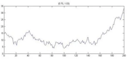
The simplest form of modeling explosive behavior is to switch at some point [τ∗T] from a ran-dom walk process to an explosive one withρ∗>1. Using 2000 replications, the power of all statistics was evaluated for different values ofτ∗andρ∗of equations (3) and (5). An example series for τ=0.70 and ρ=1.03 is presented in Figure 2. Shortly after the 0.70∗200=140th observation, it can be observed that the series shows a tendency to grow.
Table 1: Upper tail critical values for test statistics
Test statistics
Quantile supB GsupB supDFC GsupDFC supADF GsupADF
a) Asymptotic critical values
0.90 2.89 2.95 1.48 2.95 1.00 1.49
0.95 3.37 3.12 1.86 3.19 1.27 1.77
0.99 4.52 3.69 2.53 3.70 1.82 2.23
b) Finite sample critical values T = 200
0.90 2.96 3.86 1.46 3.20 1.05 1.75
0.95 3.58 4.49 1.84 3.48 1.38 2.01
0.99 4.84 5.60 2.71 4.03 1.91 2.70
c) Finite sample critical values T = 100
0.90 3.19 4.00 1.60 3.35 1.10 1.48
0.95 3.77 4.54 1.94 3.68 1.37 2.36
0.99 4.86 5.97 2.57 4.34 2.06 3.54
The critical values were computed by simulating 2000 random walk processes withy0=15 and gaussian white noise. The sample size of the asymptotic critical values was set to 2000.
size’. The numbers in these rows are the rejection frequencies of falsely rejecting the null of no bubble. At a nominal size of 5%, all values in both rows should equal 0.05. It can be seen that indeed, all numbers are around 0.05. Only the supDFC statistic seems to be sightly oversized with 7%. This might be an indication for having found critical values, which are too low. Now let us turn to the power results of the test statistics. All results have three things in common: As expected an increase inρ leads to a higher rejection frequency; An earlier break pointτ∗
Figure 2: Random walk withτ=0.70 andρ=1.03
Table 2: Rejection Frequencies on a random walk with drift Process
Test statistics
drift supB GsupB supDFC GsupDFC supADF GsupADF
a) T = 100
0.02 0.05 0.06 0.05 0.05 0.06 0.07
0.05 0.05 0.06 0.07 0.06 0.07 0.05
0.10 0.10 0.09 0.12 0.08 0.09 0.06
0.25 0.44 0.38 0.52 0.32 0.19 0.13
0.50 0.96 0.95 0.98 0.89 0.40 0.39
b) T = 200
0.02 0.05 0.04 0.06 0.04 0.04 0.06
0.05 0.07 0.06 0.10 0.06 0.05 0.06
0.10 0.19 0.13 0.21 0.14 0.09 0.10
0.25 0.78 0.71 0.85 0.62 0.26 0.27
0.50 1.00 1.00 1.00 1.00 0.40 0.63
The underlying process is a random walk with drift:yt=d r i f t+yt−1+ǫt, whereǫtis standard
Table 3: Empirical power for fixedτ∗andρ∗
Test statistics
Break point Magnitude supB GsupB supDFC GsupDFC supADF GsupADF
a) Power for T = 100
Actual size 0.06 0.05 0.07 0.06 0.05 0.05 τ∗= 0.7 ρ∗= 1.02 0.34 0.27 0.61 0.35 0.31 0.28 ρ∗= 1.03 0.58 0.50 0.79 0.62 0.57 0.58 ρ∗= 1.04 0.75 0.67 0.88 0.78 0.75 0.76
ρ∗= 1.05 0.81 0.75 0.93 0.88 0.83 0.87
τ∗= 0.8 ρ∗= 1.02 0.20 0.15 0.49 0.23 0.17 0.16
ρ∗= 1.03 0.32 0.23 0.68 0.42 0.33 0.36 ρ∗= 1.04 0.56 0.36 0.77 0.60 0.53 0.56 ρ∗= 1.05 0.60 0.44 0.86 0.72 0.63 0.71
b) Power for T = 200
Actual size 0.05 0.04 0.07 0.06 0.05 0.05 τ∗= 0.7 ρ∗= 1.02 0.69 0.62 0.79 0.69 0.63 0.67
ρ∗= 1.03 0.85 0.82 0.90 0.86 0.82 0.84 ρ∗= 1.04 0.92 0.91 0.95 0.92 0.90 0.93 ρ∗= 1.05 0.95 0.94 0.97 0.96 0.95 0.97
τ∗= 0.8 ρ∗= 1.02 0.48 0.42 0.69 0.50 0.41 0.48 ρ∗= 1.03 0.70 0.63 0.82 0.72 0.66 0.70
ρ∗= 1.04 0.81 0.77 0.89 0.83 0.77 0.83 ρ∗= 1.05 0.87 0.82 0.94 0.89 0.85 0.90 The DPG is based on equations (3) and (5). The number of replications is 2000. The rows ’Actual size’
3.3 DGP under randomly starting Bubbles
After having observed the results of explosive growth processes that were fixed in nature, the next step is to evaluate the power of the statistics on randomly starting bubbles. In order to simulate the seriesPt =Ptf+Bt one first needs to generate the market fundamentalPtf. Homm and Breitung (2011) determine this quantity as follows:
Ptf =1+rf r2f µ+
1 rf
Dt, (14)
where the dividendsDt are generated by a random walk with driftµand white noiseut
Dt=µ+Dt−1+ut. (15)
In equation (14),rf denotes the risk-free interest rate andµis the same number as in equa-tion (15). The randomly starting bubble componentBt is given by
Bt = (
Bt−1+
rfBt−1
π θt, ifBt−1=B0 (1+rf)Bt−1, ifBt−1>B0.
(16)
In this bubble processθt is an iid Bernoulli process that takes on the value 1 with probability
πand 0 with 1−π. The parameterπcan be seen as the probability that the bubble starts to grow exponentially andB0indicates the initial value of the bubbles. This value needs to be strictly
positive, otherwise negative bubbles are generated (B0<0), which would lead to negative prices
or no bubble is generated at all (B0=0).
In this thesis, I follow Evans (1991) to determine the parameters of the equations. Equation (15) is simulated usingµ=0.0375,D0=1.30 and a normally distributed noise with zero mean
and varianceσ2=0.1574. Furthermore, the interest raterf =0.05. The only parameters that are varied are the probability of a bubble to grow exponentiallyπand the initial bubble valueB0.
Figure 3 shows four processes for different values ofπandB0. The bottom right graph indicates
that a higher initial bubble value leads to a stronger growth in the series. The other three graphs show patterns of a random starting point of explosive growth.
The power results, summarized in Table 4, reveal two clear relationships: Firstly, as expected a higher value for B0 leads to higher rejection frequencies and secondly, including more
Table 4: Empirical power for randomly starting bubbles
Test statistics
Initial value π supB GsupB supDFC GsupDFC supADF GsupADF
a) Power for T = 100
B0=0.10 0.02 0.49 0.42 0.79 0.50 0.28 0.19
0.10 0.49 0.44 0.82 0.48 0.27 0.20
0.50 0.50 0.39 0.82 0.49 0.26 0.18
1.00 0.52 0.43 0.83 0.46 0.27 0.19
B0=2 0.02 0.82 0.81 0.94 0.84 0.75 0.75
0.10 0.99 0.98 0.99 0.99 0.98 0.98
0.50 1.00 1.00 1.00 1.00 1.00 1.00
1.00 1.00 1.00 1.00 1.00 1.00 1.00
b) Power for T = 200
B0=0.10 0.02 0.97 0.95 0.99 0.96 0.88 0.93
0.10 0.99 0.99 1.00 1.00 1.00 1.00
0.50 1.00 1.00 1.00 1.00 1.00 1.00
1.00 1.00 1.00 1.00 1.00 1.00 1.00
B0=2 0.02 0.99 0.98 0.99 0.98 0.97 0.99
0.10 1.00 1.00 1.00 1.00 1.00 1.00
0.50 1.00 1.00 1.00 1.00 1.00 1.00
1.00 1.00 1.00 1.00 1.00 1.00 1.00
The data was generated according toPt=Ptf+Bt wherePtf is given by (14) and (15) andBtby (16). The
Figure 3: Randomly starting Processes for differentπandB0=0.10; Bottom right withB0=2
3.4 DGP under a periodically collapsing Process
Contrary to the two previous DGPs, the following processes deal with the possibility of the pres-ence of multiple bubbles. In these DGPs it is not only possible for a bubble to burst, but also to evolve again. PSY (2012) have shown that the supADF statistic has low power in detecting multiple bubbles and they have empirically proven that the GsupADF test is superior on these instances. It will be interesting to see if the other general sup statistics improve the power of the statistics as well. The first multiple bubbles DGP to investigate is the periodically collapsing process. Evans (1991) has created the following periodically collapsing bubble model. The asset price is being computed similarly to the previous case:Pt=Ptf+κBt withκ>0, where the mar-ket fundamentalPtf is generated according to equations (14) and (15). The bubble component Bt, however, is simulated differently:
Bt+1=
(
(1+rf)BtǫB,t+1 ifBt<b h
ζ+π−1(1+rf)θt+1(Bt−(1+rf)−1ζ) i
ǫB,t+1, otherwise.
(17)
Here, the notation needs to be explained in detail. The error termǫB,t =exp(yt−τ2/2) with
Table 5: Parameters
µ σ2ofut D0 rf b B0 π ζ τ κ
0.0373 0.1574 1.3 0.05 1 0.5 see Table 6 0.50 0.05 20
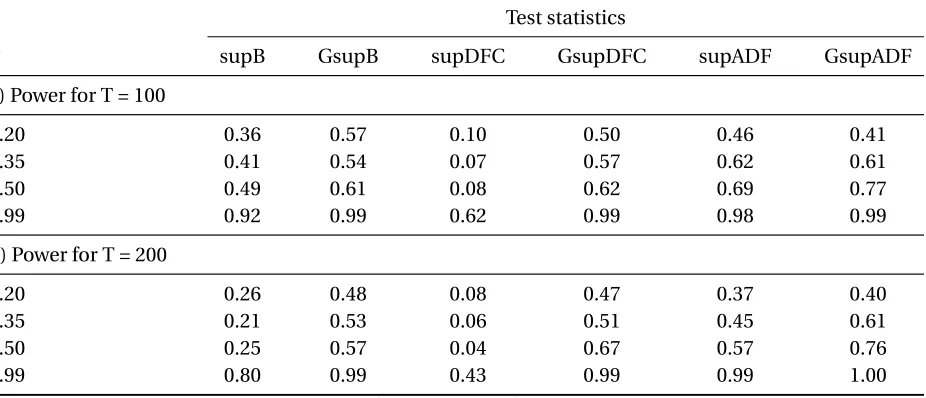
process that equals 1 with probabilityπand 0 otherwise. Figure 4 illustrates the behavior ofPt for different values ofπ. Sinceπrepresents the probability of the bubble to continue growing, we can expect longer and higher bubbles to evolve for larger values ofπ. This expectation is met by observing Figure 4. For instance, it can be seen that forπ=0.99 the bubbles take longer to eventually collapse and grow higher than for e.gπ=0.20, as in the top left graph. The presence of multiple bubbles can be witnessed, as well.
In order to simulate this periodically collapsing process all parameters have to be set first. Evans (2011) provided settings that I follow. Table 5 summarizes the parameter settings used to generate the data. The only parameter to vary isπ. All power results are reported in Table 6. Un-der this periodically collapsing process, there are two commonalities. Firstly, asπincreases, the power of all statistics tend to increase as well and secondly, contrary to the previous cases an in-crease in the sample size does not lead to higher rejection frequencies. In most cases, additional sample observations seem to have a negative impact on the power results of the statistics. One statistic particularly stands out with its results: the supDFC statistic. While the subDFC statistic performed best on single bubble DGPs, on this specific multiple bubble generating process it shows severe weakness to detect a bubble. The highest rejection frequencies in this setting have the GsupB statistic for low values ofπand the GsupADF statistic for higher values ofπ. All in all the GsupB and GsupDFC statistics performed significantly better than their sup statistics and the GsupADF statistic has higher power than its sup part on most instances, as well.
3.5 DGP under the Near-Explosive Random Coefficient autoregressive model
The Near-Explosive Random Coefficient (NERC(p)) autoregressive model belongs to the class of random-coefficient autoregressive models, in which p denotes the number of lagged depen-dent variables. In this DGP I follow Banerjee, Chevillon and Kratz (2013) and implement the following NERC(1) model:
yt=ρtyt−1+ηt, (18)
Figure 4: Periodically collapsing Processes for different values ofπ
Table 6: Empirical power for periodically collapsing bubbles
Test statistics
π supB GsupB supDFC GsupDFC supADF GsupADF
a) Power for T = 100
0.20 0.36 0.57 0.10 0.50 0.46 0.41
0.35 0.41 0.54 0.07 0.57 0.62 0.61
0.50 0.49 0.61 0.08 0.62 0.69 0.77
0.99 0.92 0.99 0.62 0.99 0.98 0.99
b) Power for T = 200
0.20 0.26 0.48 0.08 0.47 0.37 0.40
0.35 0.21 0.53 0.06 0.51 0.45 0.61
0.50 0.25 0.57 0.04 0.67 0.57 0.76
0.99 0.80 0.99 0.43 0.99 0.99 1.00
The data is generated according toPt=Ptf +Bt, wherePtf is given by (14) and (15) andBtby (17). The
Figure 5: NERC(1) Processes for different values of (φ,λ) using equations (18) and (19)
ρt=exp((φ+λTα/2ut)/Tα) (19)
withφbelonging to the set of real numbers,λbelonging to the set of positive real numbers andα∈(0, 1). Moreover,ut is a standard normally distributed variable, independent ofηt and
T equals the number of observations in the sample.
The characteristics of the resulting series of this DGP highly depend on the valuec=φ+λ2. When (c <0), the series will be weakly stationary. On the other hand, if (c ≥0), the process is not weakly stationary and will develop either processes which are stationary with fat tails or non stationary with explosive growth when (λ6=0) . At some point, these bubbles will burst and might occur consecutively. The effects of varyingφandλ, so the impact of c on the series can be observed in Figure 5. The top left graph is generated by a value of (c<0), and is supposed to be weakly stationary. Indeed, on the first sight mean and variance seem to be stable. All remaining graphs have (c>0) in common. Each of which show signs of explosive growth.
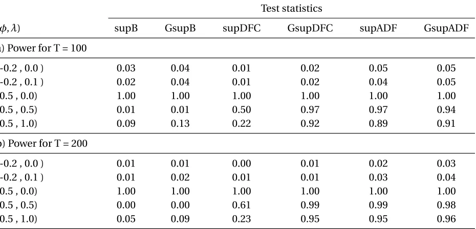
In order to test the power of the statistics I decided to generate processes that are either sta-tionary or explosive. In Table 7, the first two processes are supposed to be weakly stasta-tionary (c< 0), while the remaining three should generate bubbles. Note that the setting (φ,λ)=(0.5, 0.0) is an exponential function. Clearly, in this setting, all statistics were able to detect the exponential growth. On the weakly stationary processes, no statistic rejected the null of no bubble more often than 5%, which indicates that the statistics are slightly undersized. Turning to the last two processes, one issue stands out. Both Bhargava statistics were not able to detect a bubble in
Table 7: Empirical power for the NERC(1)
Test statistics
(φ,λ) supB GsupB supDFC GsupDFC supADF GsupADF
a) Power for T = 100
(-0.2 , 0.0 ) 0.03 0.04 0.01 0.02 0.05 0.05
(-0.2 , 0.1 ) 0.02 0.04 0.01 0.02 0.04 0.05
(0.5 , 0.0) 1.00 1.00 1.00 1.00 1.00 1.00
(0.5 , 0.5) 0.01 0.01 0.50 0.97 0.97 0.94
(0.5 , 1.0) 0.09 0.13 0.22 0.92 0.89 0.91
b) Power for T = 200
(-0.2 , 0.0 ) 0.01 0.01 0.00 0.01 0.02 0.03
(-0.2 , 0.1 ) 0.01 0.02 0.01 0.01 0.03 0.04
(0.5 , 0.0) 1.00 1.00 1.00 1.00 1.00 1.00
(0.5 , 0.5) 0.00 0.00 0.61 0.99 0.99 0.98
(0.5 , 1.0) 0.05 0.09 0.23 0.95 0.95 0.96
The data are generated using equations (18) and (19), wherebyα=0.50 andy1=10. Simulations are repeated 2000 times.
weakness in rejecting the null hypothesis. Considering the DFC statistics, the GsupDFC outper-formed its sup statistic significantly while the ADF statistics have more or less similar results. Concerning all outcomes, the GsupDFC statistic is a decent statistic to use if the underlying process shows patterns similar to the NERC(1) process on hand.
3.6 DGP under a Noncausal Cauchy linear autoregressive Process
In the past few years, researchers have recognized that it is not only possible to model a series by a standard ARMA model but also by so called noncausal autoregressive models. Contrary to ARMA models, in which current values are explained by previous values, noncausal mod-els make use of forward looking values. Gourieroux and Zakoian (2013) have investigated the modeling of bubbles using the following noncausal process:
yt =ρyt+1+ǫt, (20)
Figure 6: Noncausal Processes for different values ofρusing equation (20)
Figure 6 illustrates the behavior of the series for different values ofρ. All series are generated backwards. In other words, I fixed yT =50 and generated all other yt recursively. Values ofρ close to 0 let the bubbles appear to be shorter in their evolution and rather steep. On the other hand, whenρ→1, the length of a bubble increases.
This noncausal cauchy linear autoregressive process is different to the preceding DGPs. All processes so far fulfilled the requirement of the null hypothesis. The DGPs have all been non-stationary and changed to an explosive process. In this DGP, however, the series is non-stationary rather than a random walk and includes bubbles as it progresses. The statistics in this thesis are all based on the assumptions of theH0andH1described in the beginning of Section 2 and
therefore Gourieroux and Zakoian (2013) argued that unit root based statistics lead to wrong results and other specified tests should be used to test noncausal processes instead.
Although Gourieroux and Zakoian suggested to use other statistics to test for bubbles in noncausal models, I investigated the power of the statistics and summarized the results in Ta-ble 8. The parameter to vary wasρ. Interestingly, an increase in ρ does not really lead to a higher power of the statistics4. Conversely, higher powers are achieved whenρis either 0.50 or 0.70. Furthermore, in this underlying model all general sup statistics are superior to their sup statistics. All in all, the GsupADF statistics serves as the best detector for bubbles. Only in the ρ=0.10 setting, the GsupB and GsupDFC statistics have a higher rejection frequency. Whether the power results are trustworthy or not is a question for a different paper. It can be
Table 8: Empirical power for the Noncausal Model
Test statistics
ρ supB GsupB supDFC GsupDFC supADF GsupADF
a) Power for T = 100
0.10 0.29 0.64 0.18 0.67 0.30 0.61
0.50 0.37 0.73 0.37 0.80 0.62 0.96
0.70 0.47 0.74 0.31 0.76 0.65 0.96
0.90 0.61 0.82 0.14 0.63 0.54 0.85
b) Power for T = 200
0.10 0.22 0.61 0.03 0.54 0.19 0.43
0.50 0.27 0.68 0.13 0.76 0.54 0.90
0.70 0.28 0.72 0.13 0.76 0.64 0.95
0.90 0.35 0.76 0.03 0.64 0.61 0.90
The Data was generated using equation (20), and repeated 2000 times.
concluded, however, that the noncausal model definitely generates bubbles in all instances and that the GsupADF statistic, for instance, is able to reject the null of no bubble in over 90% for some parameter settings ofρ.
4 Application
After having computed the power of the statistics on different bubble generating processes, this section will apply the test statistics on real data. As test instances, the Internet currency Bitcoin and Japan’s main stock index Nikkei 225 are chosen.
4.1 The Bitcoin Bubble
signifi-Table 9: Results of Test Statistics under the Bitcoin series
Test statistics
supB GsupB supDFC GsupDFC supADF GsupADF
Results 2.36 2.36 0.03 5.43 6.47 6.47
a) Asymptotic critical values
90 % 2.89 2.95 1.48 2.95 1.00 1.49
95 % 3.37 3.12 1.86 3.19 1.27 1.77
99 % 4.52 3.69 2.53 3.70 1.82 2.23
The supADF and GsupADF statistics are computed by including 4 lags
cantly higher volatility compared to the U.S. Dollar5(Williams, 2014). The volatility reached its peak when the currency jumped from a price of 15$ in January 2013 to prices of over 1000$ in November the same year. This surge in the asset price can be observed in Figure 7. The chart reveals the presence of a bubble starting at approximately the 100th sample observation and a burst at around 50 observations later. The underlying data was downloaded from Datastream and one observation equals one trading day. Moreover, the time horizon covers the past two years. By comparing this graph to the processes generated in section 3, it can be seen that the first two DGPs have nothing in common with the Bitcoin series due to the fact that both DGPs do not contain bubble bursts. Furthermore, the periodically collapsing process seems to be dif-ferent in nature as well and the noncausal model DGP does not fit with its stationary character either. Hence, the only process that could possibly generate a series similar to the one on hand is the NERC(1) process. Note that the graphs illustrated in Figure 5 are only representatives for four different parameter combinations.
Before applying the test statistics on the series, I conducted two tests in order to guarantee trustworthy results. As outlined in section 3.1, the test series needs to be trend-less so that the provided critical can be used. A simple regression confirmed the insignificance of a linear trend and a constant. Furthermore, to ensure that the residuals are not serially correlated, the Schwarz Information Criterion determined the lag length of the ADF statistics to be 4. The application of all test statistics on this time series yielded the results in Table 9. Since the series contains more than 500 sample observations the asymptotic critical values are chosen in order to determine a rejection of the null hypothesis. The null hypothesis is not rejected at the 90 % threshold by both Bhargava statistics. Apparently, the variation of the interval has not led to a higher sup value in the GsupB statistic. Interesting results show the Chow type statistics DFC. While the supDFC statistic is far from rejecting the null hypothesis, the GsupDFC statistic
Figure 7: Exchange rate of Bitcoin - USD from May 2013 to May 2015
detected a bubble at the 99 % quantile. Lastly, both ADF statistics reject the null hypothesis at the 99 % quantile, as well. Therefore, considering all statistics together three statistics suggest to accept the null hypothesis while the other three reject it. Due to the fact, however, that the series is rather similar to a NERC(1) process it can be concluded that more emphasis should be based on the decision of the GsupDFC, supADF and GsupADF statistics, since these statistics showed highest rejection frequencies on NERC(1) instances. Hence, the Bitcoin series is most likely subject to the presence of a bubble.
4.2 Japan’s Bubble in the 1980s
The second test instance I chose deals with an incident that still impacts Japan’s economy signif-icantly. After world war two, Japan’s economy experienced around 30 years of extreme growth. Thanks to the Marshall Plan, an improved relationship to the United States of America and their conglomerate businesses called ’keiretsu’ it was possible for Japan to become one of the biggest exporters of manufactured products such as cars and electronic gadgets. The cash surplus re-sulting from the exports together with an appreciation of the Yen against the U.S. Dollar enabled Japan to invest in and acquire foreign firms so that it became the second largest economy in the world. This fact, financial deregulation and a lose monetary policy led to overconfidence, which yielded in soaring stock and real estate prices (Colombo, 2012). At its peak, the land beneath the Tokyo Imperial Palace was estimated to be worth as much as the state of California (Impoco, 2008) and Japan’s main stock Index, the Nikkei 225, tripled within four years to 39000 points in 1989. Ever since the bubble collapsed to 20000 points in 1990, Japan found itself in a phase of deflation and interest rates close to zero. Up until today, no intervention6of Japan’s central
Table 10: Results of Test Statistics under the Nikkei 225 series
Test statistics
supB GsupB supDFC GsupDFC supADF GsupADF
Results 1.80 3.84 0.47 5.75 4.98 4.98
a) Asymptotic critical values
90 % 2.89 2.95 1.48 2.95 1.00 1.49
95 % 3.37 3.12 1.86 3.19 1.27 1.77
99 % 4.52 3.69 2.53 3.70 1.82 2.23
The supADF and GsupADF statistics are computed by including 0 lags
bank could change these facts.
The instance to test is Japan’s stock Index, the Nikkei 225 Index. The chart of this index is drawn in Figure 8 and covers the time between 1980 and 2000. The data are plotted weekly, meaning one sample observation equals Nikkei’s weekly price and are downloaded from Datas-tream. Moreover, the underlying currency is Yen. Contrary to the Bitcoin, the Nikkei 225 Index increased over a longer period and not as steep. After the bubble collapsed at approximately the 500th observation , it followed three years of depreciation up until around the 630th observa-tion. Ever since, the series shows stationary patterns. Possibly, a similar series can be generated by a NERC(1) or a noncausal model7.
In order to test the Nikkei Index, the same specification tests needed to be conducted in advance. Again, a regression revealed insignificant coefficients for a constant and a linear trend. Moreover, no lags were needed to compensate for serial correlation. Testing the Nikkei 225 Index yielded the results reported in Table 10. In this series there is a difference in the values of the Bhargava statistics. On the one hand, the supB statistic does not detect a bubble while on the other hand, the general sup Bhargava statistic rejects the null hypothesis at the 99 % quantile. A bigger improvement shows the GsupDFC statistic compared to its supDFC statistic. Again, the supDFC statistic is not able to detect the presence of a bubble at all and the GsupDFC statistic rejects the null hypothesis at the 99 % threshold. Lastly, both ADF statistics show strong evidence of the presence of a bubble by rejecting the null hypothesis at the 99 % quantile, as well. Altogether, the results are similar to previous ones: The GsupDFC and the ADF statistics clearly rejected the null hyphosesis; The GsupB improved compared to the Bitcoin series and the subB and particularly the supDFC statistics turned out to be weak detectors for bubbles that burst. This conclusion suggests the presence of a bubble in the Nikkei Index in the time interval of 1980 until 2000.
Figure 8: Nikkei 225 Index from 1980 to 2000
5 Conclusion
This thesis is about testing for the presence of bubbles in time series. For this purpose, two new statistics are introduced, namely the general sup Bhargava and the general sup DFC statistics. Both statistics were derived by additionally varying the time interval of their sup statistics. This trick was used by PSY to create the general sup ADF statistic from the sup ADF statistic. The power of all statistics was computed on several bubble generating processes. While the sup statistics proved to be more efficient in detecting bubbles that do not burst, a different picture was drawn when inspecting the rejection frequencies on DGPs that contain multiple bubbles. Under the latter case, the GsupDFC and the GsupADF statistics performed best and are hence advised to use for application. To confirm the results, the internet currency Bitcoin and the Japanese stock Index Nikkei 225 were tested for the presence of bubbles. It turned out, that especially the GsupADF and the GsupDFC statistics reject the null hypothesis of no bubble at the 99 % quantile in both instances.
All in all, it can be concluded that even though there exist several econometric tests that can be used to detect a bubble in a time series, it is uncertain whether any policy maker would in-tervene if an asset prices is positively tested for the presence of a bubble. In the worst case they behave like Alan Greenspan, the former Federal Reserve Chairman, who said after the Dotcom Bubble in 2002:
24
MaRBLe Research PapersReferences
Banerjee, A. N., Chevillon, G., & Kratz, M. (2013). Detecting and Forecasting Large Deviations and Bubbles in a Near-Explosive Random Coefficient Model. SSRN Electronic Journal SSRN Journal.
doi:10.2139/ssrn.2322360
Colo bo, J. , Ju e . Japa ’s Bubble Economy of the 1980s. Retrieved May 03, 2015, from http://www.thebubblebubble.com/japan-bubble/
Dash, M. (2001). Tulipomania. G.K. Hall; Thorndike, ME
Diba, B. T., & Grossman, H. I. (1988). Explosive rational bubbles in stock prices?. The American Economic Review, 78(3), 520-530
Evans, G. W. (1991). Pitfalls in testing for explosive bubbles in asset prices. The American Economic Review,
81(4), 922-930
Gouriérou C., Zakoia , J.M. . E plosive bubble odelli g b o -causal process. CREST Working Paper:
2013–04
Greenspan, A. (2002, August). Economic volatility. In Remarks at a symposium sponsored by the Federal
Reserve Bank of Kansas City, Jackson Hole, Wyoming, August (Vol. 30)
Holt, J. (2009). A summary of the primary causes of the housing bubble and the resulting credit crisis: A
non-technical paper. The Journal of Business Inquiry, 8(1), 120-129
Homm, U., & Breitung, J. (2012). Testing for speculative bubbles in stock markets: a comparison of alternative
methods. Journal of Financial Econometrics, 10(1), 198-231
Impoco, J. (2008, October 18). Life after the bubble: How Japan lost a decade. The New York Times. Retrieved May 3, 2015, from http://www.nytimes.com/2008/10/19/weekinreview/19impoco.html?_r=0
Nakamoto, S. (2008). Bitcoin: A peer-to-peer electronic cash system. Consulted, 1(2012):28
Phillips, P. C., Shi, S. P., & Yu, J. (2012). Testing for Multiple Bubbles. SSRN Electronic Journal SSRN Journal. doi:10.2139/ssrn.1981976
Phillips, P. C., Wu, Y., and Yu, J. (2011). Explosive behavior in the 1990s nasdaq: When did exuberance escalate asset values?*. International economic review, 52(1):201–226