497
Available online at http://ijdea.srbiau.ac.ir
Int. J. Data Envelopment Analysis (ISSN 2345-458X)
Vol.2, No.4, Year 2014 Article ID IJDEA-00242,12 pages
Research Article
Deriving Common Set of Weights in the Presence of
the Undesirable Inputs: A DEA based Approach
M.Eynia , M.Maghboulib*
(a) Department of Mathematics, University of Payam Noor, Tehran, Iran.
(b)
Departement of Mathematics, Islamic Azad University, Hadishahr Branch, Hadishahr, Iran.
Received 10 July 2014, Revised 6 October 2014, Accepted 14 November 2014Abstract
Data Envelopment Analysis (DEA) as a non-parametric method for efficiency measurement allows decision making units (DMUs) to select the most advantageous weight factors in order to maximize
their efficiency scores. In most practical applications of DEA presented in the literature, the presented
models assume that all inputs are fully desirable. However, in many real situations undesirable inputs
are part of the production process. In order to deal with undesirable inputs, this paper changes the
undesirable inputs to be desirable ones by reversing, then a compromise solution approach is proposed
to generate a common set of weights under DEA framework. The DEA efficiencies obtained with the
most favorable weights to each DMU are treated as the target efficiencies of DMUs. Based on the
generalized measure of distance, three types of DEA-based efficiency score programming can be
derived. The proposed approach is then applied to real-world data set that characterize the performance
of seven types of chemical activities.
Keywords: Data Envelopment Analysis (DEA), Efficiency, Undesirable Input, Compromise solution.
1. Introduction
Data Envelopment Analysis (DEA) is a non- parametric technique for evaluating the relative
efficiency of a set of homogeneous decision making units (DMUs) by using a ratio of the weighted sum
* Corresponding author: [email protected]
of outputs to the weighted sum of inputs. Specifically, it determines a set of weights such that the
efficiency of a target DMU relative to the other DMUs is maximized. This flexibility in the selection of
input and output weights often causes more than one DMU being evaluated as efficient, leading to them
being unable to be fully discriminated. As the methods of DEA are run for each DMU separately, the
set of weights will typically be different for the various DMUs. Also, in some cases it may be considered
unacceptable that the same factor is accorded widely different weights. A possible answer to this
difficulty lies in the specification of a common set of weights (CWS). To derive a common set of
weights for DMUs, a number of approaches have been proposed in the DEA literature. For example,
Kao and Hwang [7] proposed the compromise solution approach to generate a common set of weights
for all DMUs. The efficiency scores calculated from the standard DEA model is the ideal solution for
each DMU to achieve. The common set of weights which is able to produce a vector of efficiency scores
closest to the ideal solution is desired. This vector of efficiency scores is called the compromise solution.
Based on the generalized measure of distance, a family of compromise solutions with parameter p,
p
1 , can be generated. As another method, Roll and Golany[10] suggested a method including
running a general unbounded DEA model to obtain different sets of weights and then taking their
average or weighted average with DEA efficiencies as the weights, maximizing the average efficiency
of DMUs and assigning low weights to less important factors and maximal feasible weights to important
ones. Chen et.al [4] proposed a linear multi –criteria programming which can be boil down to a
single-objective linear programming by combining the DEA and the compromise solution programming.
Zohrebandian et.al [12] presented a multi-objective linear programming to generate the common
weights. Also see Belton and Vickers [2] and Li and Reevese [8].in all above mentioned literatures
multiple desirable inputs were applied to generate multiple outputs. However, in some real occasions,
both desirable and undesirable inputs may be applied. The most important example of undesirable inputs
returns to recycled system process. The garbage can be considered as undesirable inputs which need to
be reconstituted and re-entered to production process. The existing DEA researches mainly deal with
undesirable outputs in four different divisions. The first group is hyperbolic measure approach, a non-
linear DEA model introduced by Fare et.al [6] using reciprocal measure to evaluate the efficiency of
undesirable outputs. Seiford ad Zhu [11] changed the undesirable outputs to be positive desirable
outputs by a linear monotone decreasing transformation. The last one is directional distance function
approach which is proposed by Chung et.al [5]. This approach evaluates and improves DMUs’
efficiency according to the given direction. The researchers have made some contributions to deal with
undesirable outputs into DEA models. However, analysts are sometimes interested in additionally
estimating the weights in presence of undesirable inputs. In this paper we aim to search one common
production process. The method for selecting common set of weights is based on the approach presented
by Kao and Hwang [8].
The structure of this paper is organized as follows. In the next section we shall introduce standard DEA
model with presence of undesirable inputs. In the section to follow the compromise solution for
generating common set of weights under the DEA framework with undesirable inputs will be applied.
Then a real-world problem is solved by the compromise solution approach to show that the developed
models can illustrate the evaluations. Conclusions are offered in section 5.
2. DEA Frameworks
Consider a set of DMUs indexed byJ. For all j{1,...,n}, DMUjuses inputs xij (i1,...,M)to produce outputsyrj (r 1,...,S). Also, for each jJ X j 0 andYj 0. The input-oriented technical efficiency ofDMUo,o{1,....,n} can be measured by the BCC model below Banker et.al., 1984) [1].
1
1
1
. .
, 1,..., ,
, 1,...., , (1)
1 ,
0 1,...,
n
j ij io j
n
j rj ro j
n j j
j Min s t
x x i M
y y r S
j n
The model (1) tries to focus on each individual DMU to select the weights attached to the inputs and outputs, and to locate the envelopment surface. A set of weights for the inputs and outputs is determined
1
1 1
1
. .
0 , 1,..., , (2)
1 ,
, 0 , 1,..., , 1,..,
is free in sign
S
r ro o r
S M
r rj i ij o r i
M i io i
r i o
Max u y u
s t
u y v x u j n
v x
u v r S i M
u
Applying model (2) each DMU is allowed to select the most advantageous weights for maximizing its efficiency score. Thus, the resulting score is the best attainable efficiency level for each DMU. In fact,
the linear model above is an equivalent form of the following fractional model. That is to say, applying
Charnes-Cooper transformation [2], model (2) is attained. The fractional model is as follows:
1
1
1
1
. .
1 , 1,..., , (3)
, 0 , 1,..., , 1,..,
is free in sign
S
r ro o r
M i io i
S
r rj o r
M i ij i r i o
u y u Max
v x
s t
u y u
j n
v x
u v r S i M
u
3. Compromise weight solution with undesirable inputs
As far as we are aware, the standard CCR and BCC model assume that all inputs and outputs can be
taken real –valued quantities. Also all consumed inputs and produced outputs are assumed desirable.
However, in some real occasions, there are undesirable inputs. For example, in garbage recycling, trash
can be considered as an undesirable input. Assume that each DMUjconsumes M desirable inputs
) ,...., 1
(i M
1 1 1 1 . .
, 1,..., ,
, 1,..., , (4)
, 1,..., ,
1,
0 , 1,...,
o n
j ij io j
n
j tj to j
n
j rj ro j n j j j Min s t
x x i M
x x t K
y y r S
j n
In whichxtj xtj v, andv is a chosen vector such that xtj 0 for all j 1,...,n.
Definition1: The optimal value of problem model (4) is called the efficiency index of DMUo. if
o1we say DMUo is (at least) weakly efficient.
Considering the dual format of model (4), we have the following linear problem:
1
1 1
1 1 1
. .
1
0 1,..., (5)
, , 0 for all , ,
is free in sign
S
r ro o r
M K i io t to i t
S M K
r rj i ij t tj o
r i t
r i t o
Max u y u
s t
v x x
u y v x x u j n
u v r i t
u
The fractional format of model (5) can be rewritten as follows:
* 1
1 1
1
1 1
. .
1 , 1,..., (6)
, , 0 for all , , is free in sign
S
r ro o r
O M K
i io t to i t S
r rj o r
M K i ij t tj i t
r i t o
u y u
E Max
v x x
s t
u y u
j n
v x x
u v r i t
Suppose that the optimal solution of model (6) is denoted by(U*,V*,
*,uo*). The objective functionof model (6) tries to determine the efficiency under the constraints that the efficiency score of all units
are less than or equal to one when the same weights are applied. The optimal objective value of model
(6) denoted by
K t to t M i io i S r o ro r o x x v u y u E 1 * 1 * 1 * * *
. This value is the best attainable efficiency level forDMUj
. Any other set of weights would result in an efficiency score which is less than or equal toEO*.
Definition 2. DMUo Is said to be efficient if the objective value of model (6) is unity,Eo* 1.
In order to generate a common set of weights for allDMUs, we can consider E* (E1*,E2*,..,En*)as target vector or ideal solution to achieve. MOLP program can be proposed to achieve the closest weights
to the ideal vector. Consequently, in presence of undesirable input a common set of weights can be
achieved from the following model:
1 1 1 1 1 1 2 1 2 2 1 1 1 1 1 1 1 1 . . . .
1 1,..., (7)
, , 0 for
S
r r o r
M K i i t t i t
S
r r o r
M K i i t t i t
S
r rn o r
M K i in t tn i t S
r rj o r
M K i ij t tj i t
r i t
u y u Max
v x x
u y u Max
v x x
u y u Max
v x x
s t
u y u
j n
v x x
u v
all , ,
is free in sign
o
In order to solve the MOLP program, the proposed approach by Kao and Hung [8] seems acceptable.
The proposed compromise method determine the closest distance between E*j and the efficiency value attainable calculated from the common weights denoted as the vectorE(u,v,). The program can have the following format:
1 1 1 1 1 1 1 1
( ) ) 1
. .
1 1,..., (8)
, , 0 for all , ,
is free in sign.
S
r ro o n
* r p p
j M K j
i io t to i t S
r rj o r
M K i ij t tj i t
r i t o
u y u
Min (E p
v x x
s t
u y u
j n
v x x
u v r i t
u
In the model above E*j is the ideal or target efficiency score obtained from model (6). In model (8) for
the smallest value of p1 , every deviation Ej Ej
*
is weighted equally. As p increases, more weights are given to the larger deviations. There are three values of p, viz., p1,2and, which have special mathematical properties and worthy of some discussion. For different values ofp, three compromise solution approaches with undesirable inputs are achieved.
1. Ifp1, model (8) is referred to as a city block measure of distance. In other words, model (8-1) finds a set of weights that results in the minimal total deviation between Ej(u,v,
) and*
j
E . The model has the formulation as follows:
n * 1 1 1 1 1 1 1 1 ( ) ( ( , )) . .
1 1,..., (8-1)
, , 0 for all , ,
is free in
S
r ro o n
* r
j M K j j
j j
i io t to i t S
r rj o r
M K i ij t tj i t
r i t o
u y u
Min (E Min E E u v
v x x
s t
u y u
j n
v x x
u v r i t
Since
n j j E 1 *is a constant, it has no effect on the optimal solution (u,v,).Thus the objective function
is equivalent to ( , , ).
1
n j
j u v E
Min
2. Ifp2, the objective function of model (8) is to find the set of weights (u,v,).which results in the shortest distance between Ej(u,v,
)andE*j. Thus it suffices to solve the following programming:2 1 1 1 1 1 1 1 ) . .
1 1,..., (8-2)
, , 0 for all , ,
is free in sign.
S
r ro o n
* r
j M K j
i io t to i t
S
r rj o r
M K i ij t tj i t
r i t o
u y u Min (E
v x x
s t
u y u
j n
v x x
u v r i t
u
As the model presents the constraints can be rewritten in the linear format as
S r M i o K t tj t ij i rjry v x x u j n
u
1 1 1
,..., 1 , 0
, but the objective function is nonlinear. For
p , the objective is reduced to minimize the maximum of individual deviations. So, model (8) can be transformed into the following programming:
* 1 1 1 1 1 1 z . .
( ) 1,...,
1 (8-3)
, , 0 for all , ,
is free
S
r rj o r
j M K i ij t tj i t
S
r rj o r
M K i ij t tj i t r i t
o
Min s t
u y u
E z j n
v x x
u y u
v x x
u v r i t
u
Forp, the objective function means that the maximal dissatisfaction of the DMUs is decreased to be minimal. However, it is better to investigate all three values of pand make a subjective judgment. Top of all, p2 seems to be better choice, because the objective function indicates the conventional Euclidean distance between the ideal target E*andEj(u,v,
). Also from the statistical point of view this deviation has the smallest variance.4. Numerical Example
The applicability of the proposed approach is illustrated by an empirical data set consisting of seven
DMUs. In order to investigate the effect of temperature on chemical instances, each unit uses two sets
of inputs: desirable and undesirable to produce two categories of outputs. Desirable inputs includes
ionic liquid and undesirable inputs consists of temperature. What’s more, higher temperature seems
more acceptable during experiment. The outputs characterized as time (calculated per min) and the
percentage of the material which yielded. Applying model (6), BCC fractional model, the efficiency
scores are obtained. Table (1) summarizes the date set.
Table1: The Chemical Data Set
DMU Desirable Input Undesirable Input Output1 Output2
1 0 40 240 56
2 5 25 75 65
3 3 40 30 75
4 10 40 10 96
5 10 25 40 89
6 10 55 8 90
7 15 40 15 88
Employing v10 to corresponding component in undesirable inputs, Table (2) presents the efficiency scores by Model (6). What’s more, this score is used as ideal or target vector in different distance
estimations.
Table2: The results for BCC model
DMU 1 2 3 4 5 6 7
*
o
E 1 0.16 0.29 0.39 1 0.43 1
It can be seen that in presence of undesirable inputs, three DMUs are satisfied in efficiency definition.
That is, their efficiency scores are unity. The objective is to find such compromise weights for both
of closeness, three distance measure are used to indicate the compromise weights. In Model (8) p represents the distance parameter. Forp1, the deviation E*j Ej is weighted equally. Hence model (8) boils down to model (8-1). Forp2, the objective is to find the set of weights which results in shortest distance between E2and E* in the conventional Euclidean space. To solve model (8) for
2
p , it suffices to solve model (8-2). Forp, the objective is to minimize the maximum of individual deviations. Hence model (8) can be transformed to model (8-3). The most prominent
characteristic features of these models is to allow each unit to select the most favorable weights in
calculating efficiency under the envelopment constraints. What’s more, referring to decision maker,
every distance measure can be selected to reflect the shortest deviation in each point of view. Table (3)
reports the results of utilizing the three proposed model to data set of Table (1). Likewise, selects the
results in Table (2) as ideal vector to compromise.
Table (3): Efficiency scores calculated from different methods of common weights
DMU *
o
E Model(8-1) Model(8-2) Model(8-3)
1
p p2 p
1 1 10.1318(1) 8.3332(1) 1.9845(1)
2 0.16 4.2518(7) 5.0760(7) 1.1445(7)
3 0.29 5.1618(6) 5.7474(6) 1.2745(6)
4 0.39 5.8618(5) 6.1940(5) 1.3745(5)
5 1 10.1318(2) 8.3332(2) 1.9845(2)
6 0.43 6.1418(4) 6.3612(4) 1.4145(4)
7 1 10.1318(3) 8.3332(3) 1.9845(3)
The associated ranking calculated from three different methods of common weights are shown in
parenthesis. As Table (3) presents efficiency score calculated from Model (8-1) the largest efficiency
score is obtained (10.1318), whereas, Model (8-2) and Model (8-3) have smaller values of 5.0760 and
1.1445. However, there is no differences between efficient units but also detect some information in
presence of undesirable inputs. The common set of weights generated from these three models are
shown in Table (4).
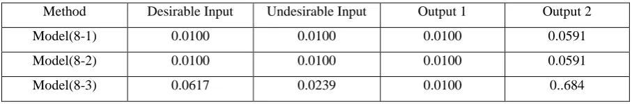
Table (4): Common set of weights from different models
Method Desirable Input Undesirable Input Output 1 Output 2
Model(8-1) 0.0100 0.0100 0.0100 0.0591
Model(8-2) 0.0100 0.0100 0.0100 0.0591
As Table (4) shows the resultant weights are same for Model (8-1) and Model (8-2). However, they
reflect the technical rates of substitution, but the results are same. As Kao and Hwang [8] argues it is
inappropriate to say which weights are correct and which are not. Also, the ranking of these three models
are consistent with those of the BCC model, indicating that the results are reasonable. The compromise
solution approach of Model(8) is to use different distance measures to generate a linear production
frontier such that the efficiency scores of the DMUs calculated from this production frontier are closest
to the target efficiency scores.
5. Conclusion
Standard DEA models suffers flexibility in selecting weights for inputs and outputs in calculating the
efficiency scores. This shortcoming of this flexibility highlights when it hampers a common base for
comparison in presence of undesirable inputs. This paper researches one common set of weights that is
the most favorable for determining the absolute efficiency for DMUs in presence of undesirable inputs.
The paper proposes the compromise solution approach to generate a common set of weights for all
DMUs. Based on generalized measure of distance, three DEA-based model are generated to obtain a
common set of weights. The practical application of this methodology is aimed at evaluating a group of
DMUs characterizes the performance of 7 real-chemical activities with undesirable inputs.
References
[1]Banker, R.J., Charnes, A., Cooper, W.W., 1984. Some models for estimating technical and scale
inefficiencies in data envelopment analysis. Management Science 30(9), 1078-1092.
[2] Belton V and Vickers SP. Demystifying DEA-A visual interactive Approach based on multiple
criteria analysis. Journal of Operation Research Society 44 (1993): 883-896.
[3] Charnes A, Cooper WW and Rhodes E .Measuring efficiency of n decision making unit. European
Journal of Operation Research 2 (1978): 429-444.
[4] Chen, Y-W. Larbani, M. Chang, Y-P. Multi objective data envelopment analysis. Journal of
Operation Research Society (2009) 60: 1556-1566.
[5]Chung, Y., Fare, R., 1995. Productivity and Undesirable Outputs: A Directional Distance Function
Approach. Discussion Paper Series No. 95-24
[6] Fare, R.,Grosskopf,S.,Lovell,C.A.K.,1989.Multilateral productivity comparisons when some
outputs are undesirable :a nonparametric approach. The Review of Economics and Statistics71,90–98.
[7] Fare, R., Grosskopf, S., Lovell,C.A.K.,Yaiswarng,S.,1993.Deviation of shadow prices for
undesirable outputs: a distance function approach. The Review of Economics and Statistics.75, 374–
[8] Kao C and Hung CT. Data envelopment analysis with common weight: The compromise solution
approach. Journal of Operation Research Society (2005) 56: 1196-1203.
[9] Li X-B and Reevese GR. A multiple criteria approach to data envelopment analysis .European
Journal of Operation Research 115 (1999): 507-517.
[10] Roll Y and Golany B. Alternative methods of treating factor weights in DEA. Omega 21 (1993):
99-103.
[11] Seiford, L.M., Zhu, J., 2002. Modeling undesirable factors in efficiency evaluation. European
Journal of Operational Research 142, 16–20.
[12] Zohrehbandian M. Makui A. Alinezhad A. A compromise solution approach for finding common
weights in DEA: an improvement to Kao and Hung's approach. . Journal of Operation Research Society