Statistical Modeling of Student Performance to Improve Chinese Dictation Skills with an Intelligent Tutor

(1)

Statistical Modeling of Student Performance to

Improve Chinese Dictation Skills with an

Intelligent Tutor

John W. Kowalski

Carnegie Mellon University [email protected]

Yanhui Zhang

The Chinese University of Hong Kong

[email protected]

Geoffrey J. Gordon

Carnegie Mellon University [email protected]

The Pinyin Tutor has been used the past few years at over thirty institutions around the world to teach students to transcribe spoken Chinese phrases into Pinyin. Large amounts of data have been collected from this program on the types of errors students make on this task. We analyze these data to discover what makes this task difficult and use our findings to iteratively improve the tutor. For instance, is a particular set of consonants, vowels, or tones causing the most difficulty? Or perhaps do certain challenges arise in the context in which these sounds are spoken? Since each Pinyin phrase can be broken down into a set of features (for example, consonants, vowel sounds, and tones), we apply machine learning techniques to uncover the most confounding aspects of this task. We then exploit what we learned to construct and maintain an accurate representation of what the student knows for best individual instruction. Our goal is to allow the learner to focus on the aspects of the task on which he or she is having most difficulty, thereby accelerating his or her understanding of spoken Chinese beyond what would be possible without such focused “intelligent” instruction.

1. Introduction

(2)

2. Pinyin Basics

Pinyin is a system of transcribing standard Chinese using Roman characters and is commonly taught to learners of Chinese at the beginning of their instruction. Most Chinese words are composed of one or more monosyllabic morphemes. Except for a few ending with the retroflex “r”[ɚ], the maximum size of a Chinese syllable is structured as CGVV or CGVC, where C stands for a consonant, G a glide, V a vowel, and VV either a long vowel or a diphthong (Duanmu, 2007: 71). While the nucleus vowel in a Chinese syllable is obligatory, the consonant(s) and glide are optional. The Pinyin system categorizes the first consonant in the Chinese syllable as an initial, and the remaining components (GVV or GVC) as the final. Standard Mandarin Chinese also uses a suprasegmental feature called lexical tone, representing the pitch contours that denote different lexical meanings (Chao, 1968).

In the Pinyin Tutor, each syllable is transcribed to Pinyin as three components: an “initial” segment (b, n, zh, …), a “final” segment (ai, ing, uang, …), and a suprasegmental “tone” (1,2,3,4,5). In total there are twenty-three initials, thirty-six finals, and five tones (Table 1). (There are 21 initials in the Pinyin system. But in the Pinyin Tutor, there are 23 because the special representations of two glides “w” and “y” are categorized as initials. The letters “w” and “y” are used respectively when the consonants are absent before the glides “i" [j], “u” [w], and “ü” [ɥ]. For the ease of computation and the generation of feedback when spelling errors occur, “w” and “y” are regarded as initials.) In terms of the tones, Chinese is defined to have four tones: high-level, rising, dip-rising, and high-falling. The underlying tones on the weak or unstressed syllables are regarded as toneless (Duanmu, 2007, 241-242). Correspondingly, the Pinyin Tutor marks the tones on stressed syllables as Tone 1 to Tone 4, and tones on unstressed syllables as Tone 5.

3. Operationalizing the Domain

To facilitate comparison and maintain coherence with other assessments, we describe the Pinyin Tutor project in terms of the evidence-centered design (ECD) framework and describe each component in terms of the Conceptual Assessment Framework (CAF) (Mislevy et al., 2006). In each of the following subsections we give a brief description of a model in the CAF, followed by how it is implemented in the Pinyin Tutor. In this paper, we discuss two versions of the Pinyin Tutor: an original version that served as a platform for testing and developing new linguistic theories with the aim of helping learners improve skills, and a subsequent machine learning (ML) based version with these same aims but also utilizing the wealth of data we collected from the original version to improve learner instruction. Where the CAF model has been modified between these two versions, in each subsection we first describe the original version followed by the changes in the new version.

(3)

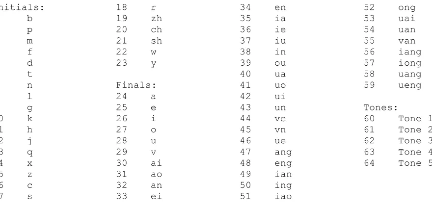
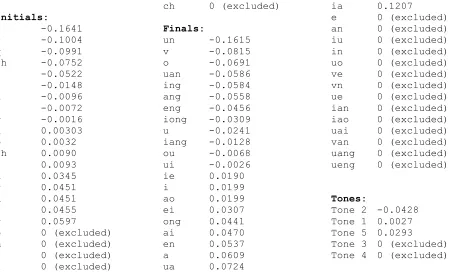
Table 1. Below are the 64 covariates along with their numeric label we used for the “basic” model (without interaction terms).

Initials: 1 b 2 p 3 m 4 f 5 d 6 t 7 n 8 l 9 g 10 k 11 h 12 j 13 q 14 x 15 z 16 c 17 s

18 r 19 zh 20 ch 21 sh 22 w 23 y

Finals: 24 a 25 e 26 i 27 o 28 u 29 v 30 ai 31 ao 32 an 33 ei

34 en 35 ia 36 ie 37 iu 38 in 39 ou 40 ua 41 uo 42 ui 43 un 44 ve 45 vn 46 ue 47 ang 48 eng 49 ian 50 ing 51 iao

52 ong 53 uai 54 uan 55 van 56 iang 57 iong 58 uang 59 ueng

Tones:

60 Tone 1 61 Tone 2 62 Tone 3 63 Tone 4 64 Tone 5

3.1 Presentation Model

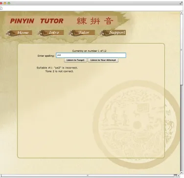
The Presentation Model answers the question “How does it look?”, describing the interface of the assessment (Mislevy et al., 2006). The Pinyin Tutor is a web-based application with an Adobe Flash front-end and server-side CGI scripts written in Perl. The operation of the presentation model is a dictation task: a Chinese word or phrase is “spoken” through the student’s personal computer speakers and the learner is asked to enter the Pinyin of that utterance. The presentation model is the same for both versions of the tutor. To produce the vast number of audio stimuli required, we recorded every pronounceable syllable in Chinese into a separate MP3 sound file (approximately 3830 in total). A unique Chinese word or phrase is then constructed by concatenating the appropriate sound files. While this technique would result in unnatural sounding speech in English, the result is adequate for Chinese speech instruction. Many instructors commented the concatenated Chinese syllables produce enunciated, deliberate sounding speech, similar to the way a teacher would speak to a beginning student. The student can listen to the target item as many times as they choose by clicking the “Listen to Target” button. Figure 1 shows a screenshot of the Pinyin Tutor in action.

The student then transcribes the item to Pinyin by typing into a text box. If the Pinyin entered is correct, the tutor congratulates the student and presents the next item in the lesson. If incorrect, the tutor gives feedback on what part of the item is incorrect and gives the student an opportunity to try again. The student can also click the “Listen to Your Attempt” button to hear the item corresponding to the Pinyin they entered. To a new learner, the differences between an incorrect attempt and the target phrase can seem quite subtle.

(4)

Figure 1. Screenshot of Pinyin Tutor giving feedback to student after hearing “ye3” but incorrectly entering “ye2” (tone incorrect).

3.2 Student Model

The Student Model answers the question “What are we measuring?” and defines latent (not directly observable) variables related to student skills and knowledge in the domain (Mislevy et al., 2006). In the first version of the Pinyin Tutor, the learner is given a set of lessons, each consisting of a set of Chinese words or phrases, typically defined by the instructor to coincide with the weekly material in their course syllabus. So, the original student model consists simply of the percentage of items answered correctly in each lesson. One weakness to this model is that the external validity of competence at this skill depends strongly on the choice of items in the lessons. For instance, if an instructor designs a set of lessons lacking practice with Tone 3, this student model may indicate a high level of mastery of items within these lessons while ignoring a fundamental skill in this domain. Another possible weakness is the large grain size of tracking student knowledge. Since this model tracks student knowledge at the level of an entire (possibly multi-syllabic) phrase, it is quite possible that it does not capture the full picture. For instance, a

(5)

component within a phrase may be easily identified if embedded in one item, but may cause difficulty if embedded in another. Despite these potential weaknesses, the pre/post tests with this student model and expertly assembled lesson sets have shown significant learning (Zhang, 2009). For example, learners enrolled in the beginning Chinese language program at a university in Pennsylvania participated in six Pinyin training sessions for one semester. The comparisons between the pretest and posttest administered before and after the training sessions showed that the students’ Pinyin spelling skills improved significantly at the level of p < .001 on all measures (word, syllable, initial, final, and tone), regardless of whether the words used as training stimuli were selected from the textbook or not (Figure 2).

Figure 2. Above are the increments of Pinyin dictation accuracy rates between the pretest and posttest in one semester. Both the group of students who used words from their textbook and the group who used general words as training items had significantly better performance after one semester of practice with the Pinyin Tutor.

Notwithstanding the successful refinement of dictation skills by using this original student model, we would still like to design a model that more accurately captures what the student knows. Rather than monitor what a student knows at the whole item level, perhaps we can design a better student model by monitoring student knowledge at the component level. That is, perhaps we can track student performance at transcribing the initial, final, and tone per syllable in context. And since we have collected much data on the types of errors students make at identifying these components, an ideal student model would take into account what we have learned about students' performance at this task. A natural way to harness both these ideas is to use this wealth of data to train a statistical model for “typical” performance at each component. Then by using these trained models and monitoring an individual student's performance at each skill, the tutor can predict the probability of a student correctly identifying a component, and use this information to sequence instructional material and estimate mastery. We discuss this student model further in section 6.

(6)

3.3 Task Model

The task model describes the material presented to the student along with the student response to it. It answers the question “Where do we measure it?” and supplies us with evidence to make claims about the student model variables (Mislevy et al., 2006). For both versions of the Pinyin Tutor, the essential components of the task model consist of the sound file(s) played through the computer's speakers and their corresponding Pinyin transcripts. The tutor only gives feedback on valid Pinyin containing the same number of syllables as the entry for the audio stimulus. We included this constraint to discourage students from entering careless or random strings of letters. The key features of the task are the initial, final, and tone components within each syllable. While the whole-item student model doesn't track student knowledge at this level, the Pinyin Tutor gives feedback on errors at the component level in both the whole-item and the component-level (ML-based) model. For example, if the Pinyin of an audio stimulus is “ci3”, whereas the student types “chi3”, the feedback will point out that the initial “ch” is incorrect. Similarly, if they typed “che2” instead of “ci3” (getting all components wrong), the feedback would be that the initial “ch” is incorrect, final “e” is incorrect, and tone “2” is incorrect.

3.4 Evidence Model

The evidence model describes how we should update our belief about the student model variables by answering the question “How do we measure it?”. Whereas the student model identifies the latent variables, the evidence model identifies the observable variables we can use to update our notions of the latent variables such as student knowledge (Mislevy et al., 2006). In the original tutor, each Pinyin phrase is thought of as one unit and isn't broken down into features. And so, the observable variables in the evidence model are correctness on the whole-item level. These observables are used to update our estimate of student knowledge by calculating the percentage of items correctly transcribed in a particular lesson.

The evidence model for the ML-based tutor defines a separate observable variable indicating correctness for each initial, final, and tone per syllable. The values of these observables are used to estimate our notion of student knowledge by feeding each into a function that computes the probability of that component being known by the student. The details of how the tutor converts these observable variables into an estimate of student knowledge are described in section 6.

3.5 Assembly Model

The assembly model describes how the tasks should be properly balanced to reflect the domain being taught and answers the question, “How much do we need to measure?” (Mislevy et al., 2006). In the assembly model of the original tutor, items the student answered incorrectly on the first try are put back into the pool of items for that lesson to be presented again; items answered correctly on the first try are eliminated from the pool. The student continues until all items in the lesson have been answered correctly. How well this assembly model reflects expertise in the domain depends strongly on how well balanced the instructor’s chosen set of items is in the lesson.

(7)

The assembly model that works with the ML-based student model operates differently. In this case, we take advantage of the rich information provided by this student model and choose items from a large pool (approximately 2300 phrases) that the student model predicts as most likely to be incorrectly transcribed by the student. Since this assembly model will give learners more practice on the components causing the student difficulty instead of re-drilling particular phrases causing difficulty, the hope is this will yield more robust learning by giving practice with these difficult parts in varying contexts (The Pittsburgh Science of Learning Center, 2013).

4. Related Work

The rapid expansion of Internet accessibility, increase in computer processor and network speeds, and recent advances in web technologies are accelerating the creation of computer-based tools for learning second languages (Davies, Otto, & Rüschoff, 2012).

4.1 Computer-Assisted Language Learning (CALL)

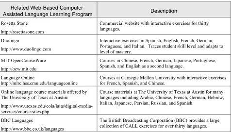
In Table 2, we list some CALL tools having qualities similar to the Pinyin Tutor. For instance, the BBC Languages website includes a “Chinese Tone Game” where the learner is presented with the audio of a Chinese phrase and is asked to choose among four choices of Pinyin which one matches the audio. Another exercise with a task similar to the Pinyin Tutor’s is included as part of the French course at Carnegie Mellon's Language Online site. In this exercise, the audio of a phrase in French is played and the student is asked to type the phrase they heard. The site then gives feedback either by letting the student know their response is correct, or by marking in red the parts of the phrase that are misspelled. While these tasks are similar in some ways to the Pinyin Tutor’s, the Pinyin Tutor is unique in that it allows students to compare the audio of their Pinyin attempts to the target, along with the very specialized feedback it gives, as described in section 3.3.

A possible critique of the Pinyin Tutor and most CALL tools in general is that they focus on an isolated subset of a language. However, to master a language, a student must be fluent in how these subsets fit together to make a whole. For instance, a particular Pinyin word can map to one or more Chinese characters, with each mapping onto different meanings. These characters in turn are combined to make new words, sometimes in non-intuitive, idiomatic ways. The “Linkit” system is an effort to create a CALL tool to illustrate these interrelationships to students of the Chinese language (Shei et al., 2012). The Linkit system consists of a database of the relationships between levels of phonology, morphology, orthography, vocabulary, and phraseology in Chinese and is constructed by experts and partially automatized by reading from existing resources on the web. Learners can use this database either in an “explore” mode to browse the relationships of Chinese language components, or in a “practice” mode where parts of the database are hidden and the student is to fill in values for these omitted components while getting feedback on their attempts. They also propose a “re-creation” exercise that uses the Linkit system to test the student on re-creating Chinese word forms and phrases based on the characters and words learned so far with the system.

(8)

Table 2.

Related Web-Based

Computer-Assisted Language Learning Program Description Rosetta Stone

http://rosettasone.com

Commercial website with interactive exercises for thirty languages.

Duolingo

http://www.duolingo.com

Interactive exercises in Spanish, English, French, German, Portuguese, and Italian. Traces student skill level and adapts to level of mastery.

MIT OpenCourseWare

http://ocw.mit.edu

Courses in Chinese, French, German, Japanese, Portuguese, Spanish, and English as a second language.

Language Online

http://mlrc.hss.cmu.edu/languageonline

Courses at Carnegie Mellon University with interactive exercises for French, Spanish, and Chinese.

Online language course materials offered by The University of Texas at Austin:

http://www.utexas.edu/cola/laits/digital-media-services/course-sites.php

Course materials at The University of Texas at Austin for many languages including Arabic, Chinese, French, German, Hebrew, Italian, Japanese, Persian, Russian, and Spanish.

BBC Languages

http://www.bbc.co.uk/languages

The British Broadcasting Corporation (BBC) provides a large collection of CALL exercises for over thirty languages.

4.2 Intelligent Computer-Assisted Language Learning (ICALL)

The ML-enhanced version of the Pinyin Tutor belongs to the family of “intelligent CALL”, or ICALL tools. Starting as its own field of research roughly in the 1990s, ICALL furthers the capabilities of traditional CALL by integrating techniques from artificial intelligence and machine learning. Techniques from these fields allow finding latent patterns in student data, parsing and generating natural language, and recognizing human speech. This enables constructing more accurate student models, giving more precise feedback, and attempts to make a more natural student-tutor interaction. ICALL tutors have made use of natural language processing (NLP), natural language generation (NLG), machine translation (MT), automated speech recognition (ASR), and intelligent tutoring system (ITS) architecture (Gamper & Knapp, 2002). In this context, the Pinyin Tutor could be considered an ITS in that it maintains a student model and provides immediate and feedback tailored to learners (Graesser, Conley, & Olney, 2012).

While there is no other ICALL system for Pinyin dictation, some ICALL systems have qualities similar to the Pinyin Tutor. Below we describe three such systems, highlighting characteristics in each analogous to those in the Pinyin Tutor.

One ITS ICALL system example is E-tutor, an online set of course materials for the German language (Heift, 2010). While the Pinyin Tutor is a tool focused on Pinyin dictation skills, E-tutor is a set of resources spanning the first three university courses in German. Both are ICALL tools that construct models to give tailored instruction addressing student strengths and

(9)

weaknesses. The student, task, evidence, and assembly models of the Pinyin Tutor are based on parsing the initial, final, and tone components of Pinyin syllables. The E-tutor models are based on errors of spelling and German grammar identified through NLP techniques. The results of E-tutor's NLP processing are used to construct phrase descriptors, indicating for instance a student error in subject-verb agreement. The E-tutor uses these results to construct an evidence model by associating with each phrase descriptor a counter that is decremented when the student successfully meets the grammatical constraint of a phrase descriptor, and incremented otherwise (Heift, 2008). The set of values for these counters are used to define E-tutor’s evidence model, which is used to tailor the lesson and feedback to each learner.

The English Article Tutor (Zhao, Koedinger, & Kowalski, 2013) was designed to help students learning English as a second language to master proper use of the English articles (“a/an”, “the”, or no article). The student models of the English Article Tutor and Pinyin Tutor are similar in that they are both informed by the results of statistical methods based on previous student data. The English Article tutor defines 33 rules necessary for the student to master English article usage. A trained model for each of these rules is used to predict the probability of applying the skill related to that rule correctly on their next attempt. Although the statistical methods used to train these models are different from those used to train models in the Pinyin Tutor, the general framework is similar. Namely, after each opportunity to apply a skill (correctly applying an article rule / correctly identifying a Pinyin component), each tutor computes the probability this skill is known and uses this information to give the student more practice on items with skills they're having most difficulty.

An ICALL system with a task model similar to the Pinyin Tutor is the ICICLE Project (Interactive Computer Identification and Correction of Language Errors) currently being developed at the University of Delaware (Michaud, McCoy, & Pennington, 2000). It is a tutor for written English with the primary aim to assist deaf students whose first language is American Sign Language. The student initializes interaction with ICICLE by submitting a piece of their English writing. The system analyzes this submission using NLP/NLG techniques to identify errors and generate feedback to help the student understand their mistakes and guide them with making corrections. The student then modifies their writing and resubmits it to ICICLE in light of this feedback, starting the cycle once again. In this sense, ICICLE's task model is similar to the Pinyin Tutor's with its cycle of student response, tutor feedback, then cycling back to the student improving their response considering the tutor’s feedback.

Our work on the intelligent Pinyin Tutor utilizes ML techniques in a way novel to the current state of ICALL. The tutor itself implements a form of knowledge tracing (KT) (Corbett & Anderson, 1995), which has been successfully implemented in many non-language tutors, but very rarely applied to ICALL tools. While KT has been used in ICALL, for instance to construct a student model of reading proficiency (Beck and Sison, 2006), our application of the statistical methods used to construct the student model for KT in a language tutor is unique. Although these techniques haven’t been applied to ICALL, they are generalizable and we anticipate they could be used to analyze and improve portions of many CALL tools. Specifically, these techniques show how to use data to construct improved student, task, and evidence models. They enable understanding what skills are important in predicting student success and how to use these important skills to give the best practice tailored to each student.

(10)

5. Identifying What Causes Students the Most Difficulty

Using data collected from the Pinyin Tutor in Fall 2008, we have approximately 250,000 training examples taken from student first attempts at an item. Each training example consists of two Pinyin phrases: the phrase presented and the student attempt at transcribing that phrase. We only include student first attempts in our analysis since second and third attempts include feedback pointing out which parts are incorrect. We do this because we do not want to include the effects of immediate feedback when training our models.

Beyond asking which items students are having trouble with, a natural question to ask is which component(s) of these items are causing the most difficulty. Are some initials, finals, or tones particularly problematic? And beyond this, we must also consider difficulties that may arise in the context in which these segments are embedded. For instance, is final “ao” easy to hear in “hao3”, but not in “bao4”? To answer these questions, we train statistical models of student performance. If we obtain a reasonably low generalization error with these models, we can gain insight to what the easy and difficult segments are as well as clues to how we can further improve instruction.

5.1 Modeling a Pinyin Syllable

A method to fit a model to our data is linear regression. We constructed our first model of a Pinyin syllable as a linear prediction with 64 covariates (one for each of 23 initials, 36 finals, 5 tones), and output whether this syllable was answered correctly. Formally, this is:

1

ˆ

y = 0+ 1x1+ 2x2 +. . .+ 64x64

where: ˆ

y 0.5(correct), y <ˆ 0.5(incorrect).

xn = 1 if feature n is present, 0 otherwise. n = coefficient for feature n.

0 = intercept.

2

= (XT_X₎ 1_XT_y

3

ˆ

y =f( 0+ 1x1 + 2x2+. . .+ 64x64)

where: ˆ

y 0.5(correct),y <ˆ 0.5(incorrect).

0 = intercept.

f(_·) = logistic function.

4

f(z) = ₁₊1_e z

5 where:

z= 0 + 1x1+ 2x2 +. . .+ 64x64

6

P

(y yˆ)2

7

P

j| j| s

where:

y indicates correctness from training data (0=incorrect, 1=correct). ˆ

y is the running predicted output of our model computed by the Lasso. (If ˆy > .5, predict correct. If ˆy _ .5, predict incorrect.)

s is a bound that can be used as a tuning parameter.

1

(1)

1

ˆ

y = 0+ 1x1+ 2x2 +. . .+ 64x64

where: ˆ

0 = intercept.

2

= (XT_X₎ 1_XT_y

3

ˆ

y =f( 0+ 1x1 + 2x2+. . .+ 64x64)

where: ˆ

0 = intercept.

4

f(z) = ₁₊1_e z

5 where:

z= 0 + 1x1+ 2x2+. . .+ 64x64

6

P

(y yˆ)2

7

P

j| j| s

where:

y is the running predicted output of our model computed by the Lasso. (If ˆy > .5, predict correct. If ˆy  .5, predict incorrect.)

1

To calculate the vector β

of model parameters, as a first method we use the normal equation (2)

to minimize the sum of squared errors.

1

ˆ

y = 0 + 1x1+ 2x2+. . .+ 64x64

where: ˆ

0 = intercept.

2

= (XT_X₎ 1_XT_y

3

ˆ

y = f( 0+ 1x1+ 2x2 +. . .+ 64x64)

where: ˆ

0 = intercept.

4

f(z) = ₁₊1_e z

5 where:

z = 0+ 1x1 + 2x2+. . .+ 64x64

6

P

(y yˆ)2

7

P

j| j| s

where:

• y indicates correctness from training data (0=incorrect, 1=correct).

• yˆ is the running predicted output of our model computed by the Lasso. If ˆy > .5, predict correct. If ˆy .5, predict incorrect.

• s is a bound that can be used as a tuning parameter.

1

(2) With this trained model, we are able to estimate the probability a syllable will be answered correctly (ŷ) by setting three covariates (xns) to 1, corresponding to the initial, final, and tone present in that syllable, and the remaining covariates to 0. We set a threshold of .5 for ŷ so that if ŷ ≥ .5 we predict a student will likely correctly transcribe this syllable, and if ŷ < .5 we predict

a student will likely incorrectly transcribe this syllable. For example, if we set to 1 the features corresponding to the initial, final, and tone of “zhi3”, our model outputs 0.6857797 ≥ .5 and so we interpret this as predicting “correct”. If however we plug in “xi5”, we get 0.4497699 < .5, and so our model predicts “incorrect” for this syllable.

(11)

Another popular method to train a classifier is logistic regression. This technique alters our model with the logistic “squashing” function. This makes it well suited for predicting student success probabilities by bounding the prediction range within [0,1]. Now instead of fitting directly to a linear equation, we fit our data to a logistic curve:

1

ˆ

y = 0 + 1x1+ 2x2+. . .+ 64x64

where: ˆ

0 = intercept.

2

= (XT_X₎ 1_XT_y

3

ˆ

y = f( 0 + 1x1+ 2x2 +. . .+ 64x64)

where: ˆ

0 = intercept.

4

f(z) = ₁₊1_e z

5 where:

z = 0+ 1x1 + 2x2+. . .+ 64x64

6

P

(y yˆ)2

7

P

j| j| s

where:

• yˆ is the running predicted output of our model computed by the Lasso. If ˆy > .5, predict correct. If ˆy _ .5, predict incorrect.

1

(3)

1

ˆ

y = 0+ 1x1 + 2x2+. . .+ 64x64

where: ˆ

xn = 1 if feature n is present, 0 otherwise. n = coefficient for featuren.

0 = intercept.

2

= (XTX) 1XTy

3

ˆ

y =f( 0 + 1x1 + 2x2+. . .+ 64x64)

where: ˆ

xn = 1 if feature n is present, 0 otherwise. n = coefficient for featuren.

0 = intercept.

f(·) = logistic function.

4

f(z) = ₁₊1_e z

5 where:

z= 0 + 1x1+ 2x2 +. . .+ 64x64

6

P

(y yˆ)2

7

P

j| j| s

where:

• yˆis the running predicted output of our model computed by the Lasso. If ˆy > .5, predict correct. If ˆy  .5, predict incorrect.

1

The logistic function is defined as:

1

ˆ

y = 0 + 1x1+ 2x2 +. . .+ 64x64

where: ˆ

0 = intercept.

2

= (XTX) 1XTy

3

ˆ

y = f( 0+ 1x1+ 2x2 +. . .+ 64x64)

where: ˆ

0 = intercept.

4

f(z) = ₁₊1_e z

5 where:

z = 0+ 1x1 + 2x2+. . .+ 64x64

6

P

(y yˆ)2

7

P

j| j| s

where:

• yˆ is the running predicted output of our model computed by the Lasso. If ˆy > .5, predict correct. If ˆy _ .5, predict incorrect.

1 (4) where: 1 ˆ

y = 0+ 1x1 + 2x2+. . .+ 64x64

where: ˆ

0 = intercept.

2

= (XTX) 1XTy

3

ˆ

y =f( 0 + 1x1+ 2x2+. . .+ 64x64)

where: ˆ

0 = intercept.

4

f(z) = ₁₊1_e z

5 where:

z = 0+ 1x1+ 2x2 +. . .+ 64x64

6

P

(y yˆ)2

7

P

j| j| s

where:

y is the running predicted output of our model computed by the Lasso. (If ˆy > .5, predict correct. If ˆy_ .5, predict incorrect.)

1

(5) The logistic function takes any value from −∞ to +∞ and converts it to a value in the range [0,1]. So unlike linear regression where ŷ has the range [−∞, +∞], we can interpret the ŷ of logistic regression as the probability of y=1 (in our case, the student correctly transcribing a syllable). We used R’s “glm” function to run logistic regression on our dataset. We obtained similar prediction accuracy for student performance with logistic regression as with linear regression.

5.2 L1-penalized Models

While the popular linear and logistic regression techniques are familiar, accessible, and often generate good models, we can construct a more accurate model with a slightly more sophisticated technique. If instead of just minimizing the error of the model to the training data as we do with linear and logistic regression, we simultaneously minimize the sum of the absolute value of the coefficients, the model can take on a number of valuable properties (Tibshirani, 1996). This sum of absolute values is referred to as the “L1-distance” or “Manhattan distance” where we sum the vertical and horizontal components of the distance between two points. This technique of simultaneously minimizing error and model coefficients is known as regularization or adding a “penalty” to a model. We can also penalize using the squared sum of the coefficients, known as the L2-distance, or Euclidean / straight-line distance. Models with an L2 penalty also have some useful properties, but do not have some that are directly useful for our current study.

The method of training a model with an L1-penalty is commonly referred to as the “least absolute shrinkage and selection operator (Lasso)”. Formally, we

(12)

Minimize:

ˆ

y = 0 + 1x1+ 2x2+. . .+ 64x64

where: ˆ

0 = intercept.

2

= (XT_X₎ 1_XT_y

3

ˆ

y = f( 0+ 1x1+ 2x2 +. . .+ 64x64)

where: ˆ

0 = intercept.

f(·) = logistic function.

4

f(z) = ₁₊1_e z

5 where:

z = 0+ 1x1 + 2x2+. . .+ 64x64

6

P

(y yˆ)2

7

P

j| j| s

where:

• yˆ is the running predicted output of our model computed by the Lasso. If ˆy > .5, predict correct. If ˆy .5, predict incorrect.

1

(6) Under constraint:

ˆ

y= 0 + 1x1+ 2x2 +. . .+ 64x64

where: ˆ

0 = intercept.

2

= (XT_X₎ 1_XT_y

3

ˆ

y= f( 0+ 1x1+ 2x2 +. . .+ 64x64)

where: ˆ

0 = intercept.

4

f(z) = ₁₊1_e z

5 where:

z= 0 + 1x1 + 2x2+. . .+ 64x64

6

P

(y yˆ)2

7

P

j| j| s

where:

• yˆ is the running predicted output of our model computed by the Lasso. If ˆy > .5, predict correct. If ˆy  .5, predict incorrect.

1

(7)

ˆ

y = 0 + 1x1+ 2x2+. . .+ 64x64

where: ˆ

0 = intercept.

2

= (XT_X₎ 1_XT_y

3

ˆ

y = f( 0 + 1x1+ 2x2 +. . .+ 64x64)

where: ˆ

0 = intercept.

4

f(z) = ₁₊1_e z

5 where:

z = 0+ 1x1 + 2x2+. . .+ 64x64

6

P

(y yˆ)2

7

P

j| j| s

where:

y is the running predicted output of our model computed by the Lasso. (If ˆy > .5, predict correct. If ˆy  .5, predict incorrect.)

1

Computing the above minimization is a quadratic programming problem and could naively be quite computationally expensive. However, the least angle regression (LARS) technique (Efron et al., 2004) provides an efficient solution.

In the lasso method, if the tuning parameter s is very large, the β’s can grow unconstrained and we are left with the usual linear regression model. But for smaller values of s, we compute a “shrunken” version of the model. This shrunken version will often lead to some of the coefficients (βis) being zero, so choosing a value for s is like choosing the number of predictors in the model (Tibshirani, 1996). This introduces the classic bias-variance trade-off. A large value for s will allow the model to grow to fit the training data as best it can, but perhaps fail to generalize to cases outside the training data set (high variance). A small s will allow the model to tune to the features that best predict output overall, and not try to fit every point in the training set. But making s too small can cause the model to ignore important features necessary for prediction (high bias).

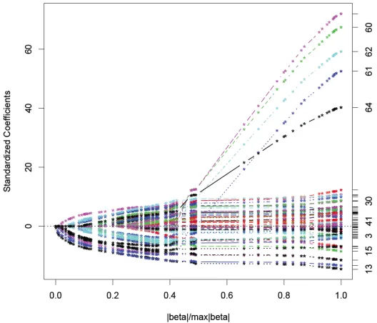
To find the optimal value for s, the authors of the LARS-lasso technique provide an R package to perform a K-fold cross-validation to measure how well a lasso model with a certain s predicts student error (Hastie et al., 2012). Typically a model will more often correctly classify an item from the dataset on which it was trained than an item from outside this set. K-fold cross-validation is a technique where we can get a better estimate on how well a model will generalize to items outside the training set. It does this by dividing the original sample into k subsets, training the model on k-1 subsets, and testing the model on the subset left out. It repeats this process k times, so that every subset is used exactly once for testing the model, and averages the prediction rate over the k tests. We set k to the often-used value of 10 and repeatedly ran 10-fold cross validation for different values of s to find the lowest s that best predicts student performance (Figure 3). We found that a model with an s that includes about 1/3 of the parameters fits as well (73.62% accuracy) as a linear regression model including all parameters (73.68% accuracy). For a graph of LARS-lasso coefficient learning progress for our 64-covariate Pinyin model see Figure 4.

J.W. Kowalski, Y. Zhang and G.J. Gordon

(13)

Figure 3. The graph above represents the K-fold cross-validated mean squared prediction error of the 64-covariate syllable model as modeled by Lars-Lasso. As described in figure 3, the x-axis represents the fraction of the abscissa values at which the CV curve should be computed, as a fraction of the saturated |beta|. Here we see that the 64-covariate model maximizes its predictive power after about 1/3 of the most important covariates (in terms of predicting syllable correctness) are included.

Figure 4. The graph above shows the coefficient learning progress of Lars-Lasso on the 64-covariate syllable model. The x-axis represents the fraction of the abscissa values at which coefficients are computed, as a fraction of the saturated |beta|. The y-axis represents the standardized values of the coefficients of each covariate. As described earlier, the Lars-Lasso method can be thought of as a linear regression with an s parameter that allows one to choose how many covariates to include in the model. The graph starts at the left with few covariates that are most predictive of whether a student will answer a syllable correctly (corresponding to using a small s). As we increase s to its maximal value (100% saturation, |beta| / max(|beta|)=1.0), we’re including all covariates, which is essentially a regular linear regression. These are the values listed on the rightmost side of the graph.

(14)

5.3 Interpreting the Trained Models

For every model discussed, we get an estimate of the probability a student will correctly transcribe the audio of a Chinese syllable into Pinyin. While the ability to estimate the difficulty of a Pinyin lesson is already quite powerful, applying the lasso gives even more insight to the skill. Since the lasso selects only the most meaningful features in predicting student performance, we are left with a parsimonious model that is easier to interpret. Another way the lasso increases interpretability is by finding a model where coefficients are small (shrinkage). This is especially true when comparing how regular linear regression can train models having correlated features. Here, the lasso avoids the situation where one correlated feature grows wildly in the positive direction, while the other grows wildly in the negative direction. While a model trained with this behavior can predict well, it may have uninterpretable coefficient values. But with our lasso-trained models, we can interpret covariates with larger coefficients as easier Pinyin skills and those with smaller ones as more difficult (Table 3). Another way to gain insight to the Pinyin transcription skill comes about by tracing the features the lasso adds as the constraint (s parameter) is gradually lifted. This algorithm trace gives us a ranking of feature importance since the lasso adds features most helpful for predicting student performance first (Table).

Table 3. Listed below are the coefficients of the basic 64-covariate syllable model learned by Lars-lasso with only the most important features present. Within each component type, rank is from hardest to easiest followed by “excluded” features that aren’t as helpful in predicting student performance.

Initials:

c -0.1641 r -0.1004 q -0.0991 zh -0.0752 z -0.0522 s -0.0148 x -0.0096 j -0.0072 y -0.0016 h 0.00303 p 0.0032 sh 0.0090 l 0.0093 k 0.0345 g 0.0451 d 0.0451 f 0.0455 w 0.0597

b 0 (excluded) m 0 (excluded) t 0 (excluded) n 0 (excluded)

ch 0 (excluded)

Finals:

un -0.1615 v -0.0815 o -0.0691 uan -0.0586 ing -0.0584 ang -0.0558 eng -0.0456 iong -0.0309 u -0.0241 iang -0.0128 ou -0.0068 ui -0.0026 ie 0.0190 i 0.0199 ao 0.0199 ei 0.0307 ong 0.0441 ai 0.0470 en 0.0537 a 0.0609 ua 0.0724

ia 0.1207

e 0 (excluded) an 0 (excluded) iu 0 (excluded) in 0 (excluded) uo 0 (excluded) ve 0 (excluded) vn 0 (excluded) ue 0 (excluded) ian 0 (excluded) iao 0 (excluded) uai 0 (excluded) van 0 (excluded) uang 0 (excluded) ueng 0 (excluded)

Tones:

Tone 2 -0.0428 Tone 1 0.0027 Tone 5 0.0293

Tone 3 0 (excluded) Tone 4 0 (excluded)

(15)

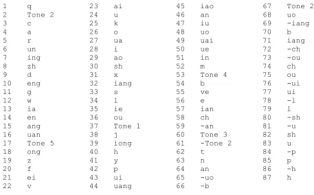
Table 4. Listed below is the sequence of lasso moves with the step number followed by the feature added to the model. Features added in earlier steps are more correlated with student performance than features added in later steps. As the constraint on the lasso is lifted and more variables are allowed, sometimes the combination of multiple features less-correlated with student performance predict better than a previously added feature. In this case the lasso removes the feature in the less constrained model. This is indicated by a minus sign in front of the feature.

1 q 2 Tone 2 3 c 4 a 5 r 6 un 7 ing 8 zh 9 d 10 eng 11 g 12 w 13 ia 14 en 15 ang 16 uan 17 Tone 5 18 ong 19 z 20 f 21 ei 22 v

23 ai 24 u 25 k 26 o 27 ua 28 i 29 ao 30 sh 31 x 32 iang 33 s 34 l 35 ie 36 ou 37 Tone 1 38 j 39 iong 40 h 41 y 42 p 43 ui 44 uang

45 iao 46 an 47 iu 48 uo 49 uai 50 ue 51 in 52 m 53 Tone 4 54 b 55 ve 56 e 57 ian 58 ch 59 -an 60 Tone 3 61 -Tone 2 62 t

63 n 64 an 65 -uo 66 -b

67 Tone 2 68 uo 69 -iang 70 b 71 iang 72 -ch 73 -ou 74 ch 75 ou 76 -ui 77 ui 78 -l 79 l 80 -sh 81 -u 82 sh 83 u 84 -p 85 p 86 -h 87 h

5.4 Toward a More Accurate Model

We have encountered technical limitations in finding models more accurate than our 64-covariate model. For instance, we were unable to use the R package to optimize the model containing all possible interaction terms between segments without running out of system memory. Shortly before the writing of this paper, we realized the existence of a new and very computationally efficient system for linear classification called LIBLINEAR (Library for Large Linear Classification) (Fan et al., 2008). With it, we were able to train a 5327-covariate model that included all main effects, plus all 2-way and 3-way interaction terms of the 64 Pinyin segments: 5327 = (64) + (23×36+23×5+36×5) + (23×36×5). We used LIBLINEAR to perform L1-regularized logistic regression to train this model. Formally, LIBLINEAR finds:

(16)

8

min P_j_| j|+CPl_i₌₁log(1 +e yi

T_x i₎

where:

is the vector of weights learned by the model.

xi is the vector representing the ith Pinyin item presented to a student.

yi = +1 if item i answered correctly, yi = 1 if item i answered incorrectly.

C >0 is a penalty parameter.

l is the number of training items.

9

t(i) =P(qt= Si | O1, O2, ..., Ot, )

where:

t(i) is the probability of being in statei at time t.

i2 {Learned,Unlearned}.

Ot is the observation of a correct/incorrect attempt at time t.

is the trained HMM for a skill.

2

(8)

8

min P_j| j|+CPl_i₌₁log(1 +e yi

T_x i₎

where:

C > 0 is a penalty parameter.

9

t(i) =P(qt =Si |O1, O2, ..., Ot, )

where:

t(i) is the probability of being in state i at time t.

i 2 {Learned,Unlearned}.

2

If βTxi > 0, the trained model predicts “correct”, “incorrect” otherwise. Using 10-fold cross

validation, we found our LIBLINEAR-trained model predicts with approximately 87% accuracy. Compared to our results with the 64-covariate model, the improvement in prediction accuracy shows there is substantial information contained in the interaction terms. In Table 5, we show some of the strongest interaction terms in predicting student performance.

6. Making the Pinyin Tutor More Intelligent

While the practice the original Pinyin Tutor version provides is valuable (Zhang, 2009), it may not be the most efficient way for students to learn, since remediation is based on the whole item, not on the particular segments of the item causing difficulty. For example, if the tutor presents the two-syllable item “ni2hao3”, but the student incorrectly types “ni2ho4”, the original assembly model will put this item back into the pool for a future re-drilling. But the student did not demonstrate difficulty with initials “n” or “h”, final “i”, or the tone in the first syllable. The student did, however, demonstrate difficulty with the final “ao”. Specifically, the student demonstrated difficulty with the final “ao”, when in the second syllable, preceded by initial “h”, with tone 3. What if we could give students more focused practice on the parts they have demonstrated difficulty? For our example, what if we could give more practice on items most similar to having a final “ao” in the second syllable, preceded by initial “h”, with tone 3? By modifying the assembly model to drill similar items instead of the exact same item, we also avoid the possibility that the learner relies on a mnemonic crutch such as “when I hear ‘ni2hao3’ be sure to mark the syllables as Tone 2 and Tone 3”.

To achieve this type of behavior, we augmented the Pinyin Tutor’s assembly model with knowledge tracing (Corbett et al., 1995). To implement knowledge tracing, the subject to be taught is broken down into a set of skills necessary for the student to master in order to master that subject. As the student works through the tutor, knowledge tracing continually estimates the probability a student knows a skill after observing student attempts at the skill. This estimate allows the tutor to give more practice on items with skills where the student is having the most difficulty. This technique has shown to be effective in domains where the set of necessary skills can be clearly defined, such as the rules necessary to solve an algebra problem (Koedinger et al., 1997) or a genetics problem (Corbett et al., 2010), or to prove geometric properties (Koedinger et al., 1993).

(17)

Table 5. Some of the most important coefficients of the 5327-covariate model learned by LIBLINEAR. Within each interaction type, we first show ten terms most important in predicting an incorrect student response (strongest negative), followed by ten terms most important in predicting a correct student response (strongest positive).

Strongest Negative Initial_Final Interaction Terms

h_a -5.40

k_i -4.21

k_o -3.85

w_a -3.83

g_o -3.81

sh_o -3.72 zh_o -3.49 d_en -3.31

g_i -3.16

k_uan -3.08

Strongest Positive Initial_Final Interaction Terms

j_ie 5.74

j_ing 4.63

h_uo 4.49

c_ai 4.49

j_ia 4.46

j_ue 4.15

y_in 4.10

y_e 3.98

y_i 3.97

l_un 3.93

Strongest Negative Final_Tone Interaction Terms

o_4 -3.45

o_2 -3.30

o_1 -2.86

ue_3 -2.86

o_5 -2.59

e_3 -2.31

ing_3 -2.16

v_2 -2.08

ua_3 -2.07 ao_2 -1.72

Strongest Positive Final_Tone Interaction Terms

ie_5 2.41 iang_5 1.97 uang_5 1.88 e_5 1.67 uan_1 1.53 iang_3 1.38 eng_1 1.37 i_4 1.28 o_3 1.27 ai_5 1.22

Strongest Negative Initial_Tone Interaction Terms

k_2 -4.38

m_1 -4.34

g_2 -4.11

n_1 -3.75

q_4 -3.75

ch_4 -3.72

y_1 -3.68

r_1 -3.61

x_4 -3.46

x_2 -3.27

Strongest Positive Initial_Tone Interaction Terms

d_3 2.82

g_3 2.06

b_5 1.60

w_2 1.36

l_5 1.23

n_3 1.01

m_5 0.98

sh_5 0.90

b_3 0.85

s_5 0.66

(18)

However, formally defining the set of skills necessary for learning a language is difficult (Heilman & Eskenazi, 2006). Learning a language requires the student to master vocabulary, grammar, syntax, cultural conventions, and pronunciation. In addition, many of these skills are context sensitive and have various exceptions. Given this complexity, there are very few CALL tutors that implement knowledge tracing. It is feasible though to define a set of skills for certain subsets of a language. The Pinyin Tutor defines a reasonably sized set of skills necessary for mastery based on the values of the three component types in each syllable. Below, we will also consider a larger set of skills based on interactions between component types.

Our implementation of knowledge tracing trains a Hidden Markov Model (HMM) for each of these skills and uses the HMM to calculate the probability the skill has been learned by the student. Knowledge tracing via HMMs can be viewed as complementary to the regression techniques above (linear regression, logistic regression, and the lasso): we can use the regression techniques to discover which skills or skill combinations are important to trace, as well as to initialize knowledge tracing (as described below). Then, we can use knowledge tracing to track individual student learning in real time. Linear regression, logistic regression, and the lasso give us interpretable models providing insight to how we may better improve instruction—for example, the lasso can tell us which skills or skill combinations are important to train. But, incorporating these models directly into the tutor to implement knowledge tracing is not straightforward: these models do not adapt to the actual performance of the current student. There are variants of our logistic regression model that do adapt to observed performance (Chi et al., 2011; Pavlik et al., 2009); however, the HMM is the only one of the models mentioned here that truly treats the student’s performance as evidence about a latent knowledge level that evolves over time. For example, observing “correct, correct, correct, incorrect, incorrect, incorrect” is not the same as “incorrect, incorrect, incorrect, correct, correct, correct”; in the HMM these sequences lead to different predictions about student knowledge, while in the other models mentioned above they do not.

6.1. Hidden Markov Model Basics

A Hidden Markov Model is a statistical model that represents a Markov process with “hidden” state (Rabiner, 1989). A Markov process can be thought of as a finite state machine where transitions between states are assigned probabilities and the probability of transition to a state at time t+1 depends only on the state the machine is in at time t. The “hidden” part is that we are not able to directly observe what state the machine is in currently, just the output dependent on the current state. The output symbols are assigned a different probability distribution in each state.

6.2. Hidden Markov Model Application

We create an HMM for each skill necessary to master our Pinyin transcription task. For our first model, we'll train an HMM for each of the 64 segments the Pinyin Tutor recognizes. We can later supplement these basic 64 skills with a subset of the skills representing the interactions between each pair of features (initial-final, initial-tone, and final-tone). To choose a subset from the 64 + 23×36 + 23×5 + 36×5 = 1187 HMMs, we can use the lasso to identify

(19)

the ones that best predict student performance. That is, we can trace only the skills and skill combinations that correspond to regression coefficients that lasso identifies as nonzero.

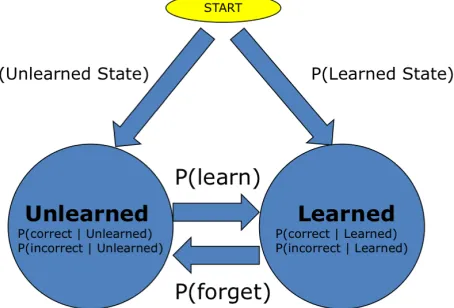
As shown in Figure 5, the HMM for each skill has two states: Learned (L) and Unlearned (U). In each of these hidden states, we are able to observe whether a skill is answered correctly (C) or incorrectly (I). The transition probabilities between each state are:

- P(learn), the prior probability of transitioning (U)à(L) at each step given that we start at (U).

- P(forget), the prior probability of transitioning (L)à(U) at each step given that we start at (L).

Conditional observational probabilities within each “hidden” state are:

- P(slip), the probability making an error even if the student is in the (L) state. - P(guess), the probability of guessing correctly even if the student is in the (U) state.

Figure 5. Hidden Markov Model representation (one for each Pinyin skill).

With the structure (states and transition paths) of the HMMs defined, we calculate the transition and conditional observation probabilities for the two states. One way to approximate transition probabilities is via the Baum-Welch algorithm, an Expectation-Maximization method that makes use of the forward-backward algorithm, a special case of belief propagation tuned to HMMs (Rabiner, 1989). We can use a single set of four parameters for all skills, or we can train separate models for each skill. Alternatively, we can use our regression models to provide priors for each skill’s parameters, or to group skills by difficulty and share parameters within each group. The more difficult skills are the ones that have larger negative coefficients.)

Again using the data collected from the Pinyin Tutor in the Fall 2008 semester and considering only student performance on their first attempt, we have approximately 250,000 student-tutor interactions for training our Pinyin skill HMMs via the Baum-Welch algorithm. To evaluate these models, we need to use them in the context of the Pinyin tutor, described in the next section.

(20)

6.3. Using Trained HMMs to Estimate Student Learning State

With HMMs trained for each skill, we are now able to estimate the probability a skill is in the Learned or Unlearned state after observing correct/incorrect attempts for that skill as the student works through the tutor lesson. Arriving at this estimate from a trained HMM is what Rabiner refers to as “Problem 2” of HMM applications (Rabiner, 1989). Namely, given an observation sequence, O, (of correct/incorrect responses) and an HMM, λ, for the skill, we

want to know the probability we are in a state Si ((U) or (L)) at time t. Formally, we want:

min _j| j|+C i=1log(1 +e yi xi)

where:

9

t(i) =P(qt =Si |O1, O2, ..., Ot, )

where:

t(i) is the probability of being in state i at time t.

i 2 {Learned,Unlearned}.

2

(9)

min P_j_| j|+CP_il₌₁log(1 +e yi xi)

where:

yi = +1 if item i answered correctly, yi = 1 if itemi answered incorrectly.

9

t(i) =P(qt =Si |O1, O2, ..., Ot, )

where:

t(i) is the probability of being in state i at timet.

i _{2 {}Learned,Unlearned_}.

2

Using the probabilities of being in the Unlearned state for each skill, we combine the probabilities of each feature present in an item being in the Unlearned state and base our selection of the next item to present on this calculation. Our aim is that by choosing items with highest average probability of being in the Unlearned state, the tutor will tailor instruction for the student precisely on skills he or she is having the most difficulty. Our ultimate goal is to get the students to a certain level of mastery much faster than the previous tutor model.

Incidentally, this approach may not be ideal for all domains. For Pinyin transcription, a student has some chance at success with the most difficult skills. However, this will not work well in domains where there is little to no chance for the student to succeed at the most difficult skills. Here, one could imagine restricting to a pool of easier items for novice students, then gradually including the more difficult items.

A practical aspect of using HMMs is that HMM-based knowledge tracing takes a trivial amount of processing time. This is very important when constructing a web-based tutor, where long pauses to choose the next Pinyin phrase are unacceptable.

A full analysis of our learned HMMs would require a study of student learning gains: we would use the HMMs in the context of the Pinyin tutor to aid problem selection, and measure the resulting student performance over time. We are in the process of conducting a pilot study of this form. However, to illustrate the performance of the learned HMMs, as well as to make clear how they are used in the tutor, we show the HMM computations for six skills after observing the sequence: 01011 (incorrect, correct, incorrect, correct, correct). For comparison, in each group of two skills, we show the HMM predictions for a skill classified as easier by our lasso analysis, followed by a skill the lasso classifies as more difficult.

(21)

Initial “w” (lasso coefficient = +0.0598):

P((“w” correct on next attempt) | (“w” observations=01011)) = 0.8512 Initial "c" (lasso coefficient = -0.1641):

P((“c” correct on next attempt) | (“c” observations=01011)) = 0.6861

Final “ia” (lasso coefficient = +0.1207):

P((“ia” correct on next attempt) | (“ia” observations=01011)) = 0.7268 Final “un” (lasso coefficient = -0.1616):

P((“un” correct on next attempt) | (“un” observations=01011)) = 0.6874

Tone 5 (lasso coefficient = +0.0293):

P((“tone 5” correct on next attempt) | (“tone 5” observations=01011)) = 0.7393

Tone 2 (lasso coefficient = -0.0429):

P((“tone 2” correct on next attempt) | (“tone 2” observations=01011)) = 0.7045

While the skills the lasso classified as more difficult have a lower probability of correct in these HMM sequence examples, in general this may not always be the case. For instance, an HMM can be trained on a skill such that the probability of transferring from the unlearned state to learned state (P(learn)) is very high, while being classified as “difficult” by the lasso. This can occur if the training sequence has many incorrect attempts (pushing the lasso estimate lower), but has the correct attempts preceded by almost all the incorrect attempts (pushing the HMM’s estimate of P(learn) higher).

7. Conclusions and Future Work

Pinyin transcription is a fundamental task for beginning students of Chinese. We have presented a novel, detailed analysis of student performance on this task. Our aim is to illuminate in detail what students find most difficult at this task, provide insight for future language research, as well as help guide building more effective tutors.

Since the Pinyin Tutor will now be keeping track of the current level of each skill for each student, we can provide teachers and students with highly detailed reports of their progress. For the first time, learners using the Pinyin Tutor will know precisely what sounds and Pinyin spelling they are having most trouble with and can pay more attention to these skills in the classroom and homework assignments.

So far, we have trained our models using data across all students. But it may be more beneficial to train models on subsets of students, e.g., considering the students’ native language. Many studies on the acquisition of second language phonology (elemental sounds) have demonstrated that the transferred features from the native language phonology are most difficult to be unlearned (Best, 1995; Flege, 1995; Flege and Mackey, 2004; Major, 2001). The error analysis on the incorrect Pinyin entries during dictation trainings showed that an

(22)

individual’s first language significantly influences the type of errors they make (Zhang, 2009). For example, English speakers have problems differentiating Tone 2 and Tone 3, whereas Cantonese speakers often confuse Tone 1 with Tone 4. Therefore, if the user’s first language can be set as a parameter for Pinyin practice, the tutor can choose the corresponding HMMs trained on data from students with the same native languages.

We are currently preparing a study to compare learning rates between the original and intelligent Pinyin Tutor versions, measuring performance at randomly selected Pinyin dictation tasks delivered at regular intervals throughout the semester.

Acknowledgements

The Pinyin Tutor began development under the direction of Dr. Brian MacWhinney as part of Yanhui Zhang's doctoral thesis at Carnegie Mellon University. This material is based upon work supported by the National Science Foundation under the grant for the Pittsburgh Science of Learning Center, Grant No. SBE-0836012. Additional support is from the Direct Grant for Research 2009-10 from the Chinese University of Hong Kong, project code 2010347, “Robust Online Pinyin Refinement Training for Cantonese Speakers”.

References

BECK,J.E.,&SISON,J. 2006. Using knowledge tracing in a noisy environment to measure

student reading proficiencies. International Journal of Artificial Intelligence in Education, 16(2), 129-143.

BEST,C.T. 1995. A direct realist view of cross-language speech perception. In W. Strange

(Ed.), Speech perception and linguistic experience: Issues in cross-language research (pp. 171–204). Baltimore: York Press.

BOURGERIE, D. S. 2003. Computer aided language learning for Chinese: A survey and

annotated bibliography. Journal of the Chinese Language Teachers Association, 38(2), 17-47.

CASELLA, G. AND BERGER, R. L. 2002. Statistical Inference (2nd. Edition) Duxbury Press,

Pacific Grove: California.

CEN, H. 2009, Generalized Learning Factors Analysis: Improving Cognitive Models with

Machine Learning. Unpublished doctoral dissertation. Carnegie Mellon University, Pittsburgh, PA.

CHAO,Y-R. 1968. A Grammar of Spoken Chinese. Berkeley & Los Angeles: University of

California.

CHI, M., KOEDINGER, K., GORDON, G., JORDAN, P., AND VANLEHN, K. 2011. Instructional

factors analysis: A cognitive model for multiple instructional interventions. Proceedings of the 4th International Conference on Educational Data Mining (EDM 2011). pp. 61-70.