A Novel ICA-based Estimator for Software Cost
Estimation
Behrouz Sadeghi1, Vahid Khatibi Bardsiri2, Monireh Esfandiari3, Farzad Hoseinzadeh4
Received (2015-07-11) Accepted (2015-10-17)
Abstract — One of the most important and valuable goal of software development life cycle is software cost estimation or SCE. There have been proposed so many models using heuristic and meta-heuristic algorithms to do machine learning process for SCE. COCOMO81 is one of the most popular models for SCE proposed by Barry Boehm in 1981. However COCOMO81 is an old estimation model, it has been widely used for the purpose of cost estimation in its new forms. In this paper, the Imperialism Competition Algorithm (ICA) has been employed to tune the COCOMO81 parameters. Experimental results show that in the separated COCOMO81 dataset, ICA can estimate the COCOMO81 model parameters such that
the performance parameters are significantly improved. The proposed hybrid model is flexible
enough to tune the parameters for any data sets in form of COCOMO81.
Keywords - DCOCOMO81, software cost estimation, accuracy, meta-heuristic, imperialism competition algorithm.
I. INTRODUCTION
M
anaging software plan and development process is one of the most challenging issuesin the field of software development scheduling
so that, time and human resources handling are those of the most important role which is called cost estimation. In fact SCE has an impressive and remarkable role in software development life cycle. From the beginning of the 1940s that the software systems concepts are introduced, SCE was also a vital and challenging process. Also the accuracy is very important for software developers and costumers because it is very useful in generating some proposals, making contracts, scheduling and controlling [1]. So that the accuracy of SCE process needed to be improved. There for, overestimating or underestimating the cost of software application can cause some
destructive effects on the whole project lifecycle.
Because accuracy is very important, in the last three decades there have been proposed many models for SCE although it is in its infancy. In
this paper the words cost estimation and effort
estimation are used interchangeably. Studying the previously done research works show that although there are some good results but they are not as acceptable as it should be[2],[3]. One of the methods which is recently very popular in improving the accuracy of SCE is using some heuristic and meta- heuristic optimization algorithms. All these algorithms tries to optimize the process of SCE. It will be discussed in section three.
In this experimental research work the ICA meta-heuristic optimization algorithm has been used to minimize the MMRE of SCE on COCOMO81 software cost estimation model. 1,3- Tayabad Unit, Payam Nour University of Khorasan
Razavi
The rest of this paper is organized as follow. Section two presents related works. In section
three firstly the COCOMO81 is briefly introduced
and then the ICA is presented. In section four, the proposed model is described in details and
performance analysis is presented in section five. And finally in section six, conclusion and future
works are presented.
II. Related work
Artificial intelligence techniques have been
used vastly in the last few years to optimize so
many problems in the vast majority of all kinds of
sciences, especially computer science. Although
these intelligent techniques seem to have so many
particular advantages, but recent studies mostly
focus on using hybrid techniques to benefit all the advantages together. There have been significant efforts put in to the researches on SCE models
using heuristic and meta-heuristic methods. In
this kind of techniques, once the algorithm has been started, it must be firstly trained by some examples, specially some large historical project
datasets are needed in this phase of the algorithm to train it accurately. Then the model iterates on its training part of the algorithm with the training data prepared for, and automatically tune the
problem specified parameters and finally depends
on some ending conditions like maximum number of iteration or convergence of the model parameters to an optimized point or achieving
to a predefined goal or even some user defined hybrid conditions, the model finishes its training
part. Now it’s the time to present some new data as test data to the algorithm, to predict the corresponding target. This part of the algorithm is known as test part.
GA-LR and GA-NLR hybrid models have been proposed for the SCE and carried out on the
NASA60 Dataset with 60 projects, COCOMO81 Dataset with 63 projects, and on NASA93 with 93 projects. The degree of MMRE on NASA60
Dataset is respectively 0.48 and 0.43 in GA-LR model in the training and testing; the same factor is respectively 0.42 and 0.2 in the GA-NLR model [4]. The degree of MMRE on COCOMO81 Dataset is respectively 0.46 and 0.35 in the training and testing steps in GA-LR model; this factor is respectively 0.44 and 0.37 in the GA-NLR model. The results show that hybrid models have a lower accuracy value of MMRE in comparison with GA, Linear Regression (LR)
and Non-Linear Regression (NLR) models. PSO-FCM and PSO-LA hybrid models have been proposed for the SCE using NASA60 Dataset.
Estimating effort using PSO [5] Parameters which influence effort estimation have been investigated
using PSO. Evaluation was conducted on
KEMERER Dataset with 15 projects. The results
show that the value of MMRE in the proposed
model equals 56.57; it is 245.39 in the COCOMO
model. GA and Scatter Search (SS) hybrid model was evaluated on NASA60 and NASA93 Datasets [6]. The value of MMRE in the hybrid model for NASA60 and NASA93 Datasets is respectively 7.56 and 23.85. The value of MMRE in GA model on NASA60 and NASA93 Datasets is respectively 19.63 and 36.51. The value of MMRE in SS model is respectively 15.21, 29.15 on NASA60 and NASA93 Datasets. The results show that the hybrid model has reduced the value of MMRE to respectively about 3.92 and 2.46 on NASA60 and NASA93 Datasets compared with COCOMO81[7].
GA and Artificial Immune System (AIS)
hybrid model has been assessed on NASA60 Dataset [8]. The value of MMRE in AIS, GA, and the hybrid models is respectively 18.20, 15.14 and 12.44.
A hybrid of Firefly Algorithm (FA) and GA
model is proposed for SCE using NASA93 Dataset. Using elitism operation GA attempts to
find the best answer for effort factors, evaluate it in fitness function and present a solution with the lowest value of error as the final answer. The
results show that the value of MMRE is 58.80 in the COCOMO model and respectively 38.31
and 30.34 in GA and FA models; it equals 22.53
in the hybrid model. Comparisons show that
the hybrid model has increased the efficacy of
estimation accuracy to about 2.88% compared with COCOMO model. The Liner Regression
(LR), Artificial Neural Network (ANN), SVR and (KNN) K Nearest Neighbors techniques
have been utilized for SCE [8].Also prediction accuracy on the tested data is respectively 60%, 95%, 80% and 60% in LR, ANN, SVR and KNN models.
III. Constructive Cost Model (COCOMO) and Imperialism Competition Algorithm (ICA)
In this section firstly a brief description
Algorithm (ICA) is explained.
1. COCOMO
The Constructive Cost Model (COCOMO) is an algorithmic software cost estimation model developed by Barry W. Boehm (1981) [9]. The model uses a basic regression formula with parameters that are derived from historical
project data and current project characteristics.
COCOMO consists of a hierarchy of three levels
[10]. The first level, Basic COCOMO is good for quick, early, rough order of magnitude estimates
of software costs, but its accuracy is limited due
to its lack of factors to account for difference in project attributes or cost drivers. Intermediate
COCOMO takes these Cost Drivers into account and Detailed COCOMO additionally accounts
for the influence of individual project phases
[11]. Basic COCOMO computes software
development effort as a function of program
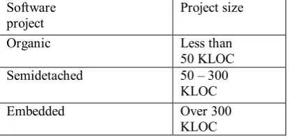
size which is expressed in estimated thousands of source lines of code [12]. COCOMO applies to Organic, Semi-detached and Embedded sorts
of projects to classify complexity of the system.
A brief description of these modes is given in Table1.
Table 1: Three Types of software projects in COCOMO
Software
project Project size
Organic Less than
50 KLOC
Semidetached 50 – 300
KLOC
Embedded Over 300
KLOC
In the basic COCOMO equations, the parameters effort Applied, development time and people required are of interest. Intermediate
COCOMO computes software development
effort as function of program size and a set of cost drivers that include subjective assessment of product, hardware, personnel and project attributes. The product of all effort multipliers results in an effort adjustment factor (EAF). The COCOMOI model takes the form of Eq. (1).
𝐸𝐸𝑓𝑓𝑓𝑓𝑜𝑜𝑟𝑟𝑡𝑡ൌ𝑎𝑎 ∗ 𝑆𝑆𝑖𝑖𝑧𝑧𝑒𝑒𝑏𝑏 𝐸𝐸𝑀𝑀 𝑖𝑖
ͳͷ
𝑖𝑖ൌͳ
Eq. (1)
Where a and b are two factors that can be set
depending on the details of the developing company and 𝐸𝐸𝑀𝑀𝑖𝑖 is a set of effort multipliers,
see Table 2.
Table 2: Overview of the COCOMOI Multipliers
EMi Description Impact
acap Analysts capability
Positive Impact: Increasing these factors results in a decreased effort
Convex relation pcap Programmers
capability aexp Applications
experience modp Modern
programming practices
tool Use of
software tools vexp Virtual
machine experience
lexp Language
experience sced Schedule
constrain
stor Main
memory
constrain Negative
Impact: Decreasing these factors results in an increased effort
data Data base
size time Time
constrain for cpu
turn Turnaround
time
virt Machine
volatility
cplx Process
complexity
rely Required
software reliability
2. Imperialist Competitive Algorithm
as the imperialist, and the others are supposed to be the colonies [15]. Assimilation policies and colonial rivalries are two main policies of this algorithm. At the beginning of the algorithm an array of the optimization variables is created which is known as a country or in some cases it is known as the screw. Each country itself has
some unique features such as economics, culture,
politics, language, and etc. The production vector
of these features or characteristics is as the Eq.
(2) in which pn is the nth characteristics of the country.
Country = [p1,p2 ,...,pn] Eq. (2)
In optimization problems the main goal is to
find the best country. So the first thing to find is to determine the cost of all the countries using Eq. (3).
Those countries which have the best set of parameters should be selected as imperialist. According to the calculated cost, only a certain number of countries are considered as colonies and the others are supposed to
be empires. In the first stage, based on the Eq. (4) the power of imperialist is defined as the total cost of its
own colonial state plus a percentage of the average cost of colonies. For each imperialist, total power T. Cn is related to the first stage.
Cost=f (country)= f(p1,p2 ,….,pn) Eq. (3)
T.Cn= Cost(imperialist)+ξ*mean{Cost (colonies
of impire_n )}
Eq. (4)
Depends on its power, each imperialist controls a number of countries. The main part of this algorithm is composed of assimilation policy and colonial competition. Regarding to absorption or assimilation policy, the imperialists countries try to destroy these nations using methods such as imposing their language and characteristics of their country on the colonies, abolishing the language and culture of the colony. In this strategy, this policy is done moving the
colonies to the imperialist according to the Eq. (5) and Eq. (6).
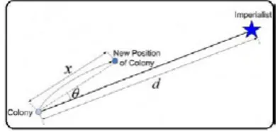
X~U (0,β*d) Eq. (5)
θ~U (-γ,γ) Eq. (6)
It can be understood from Figure 1 that a colony can move directly toward its emperor or
indirectly as seen in Figure 2.
Figure 1: a colony moving towards its colonial in a direct line.
Figure 2: a colony moving towards its colonial with a
deviation θ
In Eq. (5), if d is considered to be the distance
between a colony country and its’ colonizer then the colony movement toward the location of imperialist would be x. Of course each colony
can move through angle of θ which is called time angle and is estimated with respect to Eq. (6). Although, the movement of x and angle θ is determined randomly. Normally, the θ angle is uniformly in the interval [-γ,γ] and x momentum is estimated uniformly in the interval [0, β*d]. Values of γ and β are known as algorithm
parameters in ICA. During the algorithm, if a colony gets more power than its colonizer, then the colonizer would be replaced by that colony. In each iteration step of the algorithm, competition
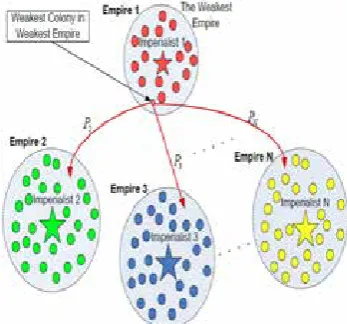
is confirmed among the colonists. Model of ICA
is shown in Figure (3).
According to Eq. (7) if a colonizer or an
imperialist has some power less than the others, it may lose one of its colonies. Based on this relation T. C_n is the total power of each imperialist and N. T. C_n is the normalized total cost. Possible appointment of a new colony to each of the colonizers is proportional to the colonial power and possible takeover by empire
is n and it is equal to (p_(p_n )) that achieved from Eq. (8). If somehow, an imperialism doesn’t
Figure 3: Imperialistic Competition
Initially, the competition between colonizers
to seize colonies is specified by T. C_n and then it is normalized by the Eq. (7) [6].
N. T. Cn = T. Cn –max{ T. Ci} Eq. (7)
Eq. (8)
The process of colonial division among empires is based on the probabilistic situation
and is represented as a vector P in the Eq. (9).
P= [ 𝑝𝑝𝑝𝑝ͳǡ𝑝𝑝𝑝𝑝ʹǡ𝑝𝑝𝑝𝑝͵ǡ𝑝𝑝𝑝𝑝Ͷǡ…Ǥ ǡ𝑝𝑝𝑝𝑝𝑛𝑛𝑖𝑖𝑚𝑚𝑝𝑝 ] Eq. (9)
In the Eq. (10), size of vector R is equal to
the size of vector P and the elements are some random number s uniformly distributed in the interval [0,1].
R=[r1,r2,r3,…,rnimp]; r1,r2,r3,…,rnimp ≈U(0,1)
Eq. (10)
According to the Eq. (11), vector D is formed
by subtracting the values of vector P from vector R.
D=P-R=[ 𝑝𝑝𝑝𝑝ͳ-𝑟𝑟ͳǡ𝑝𝑝𝑝𝑝ʹ-𝑟𝑟ʹǡ𝑝𝑝𝑝𝑝͵-𝑟𝑟͵,…,𝑝𝑝𝑝𝑝𝑛𝑛𝑖𝑖𝑚𝑚𝑝𝑝]-𝑟𝑟𝑛𝑛𝑖𝑖𝑚𝑚𝑝𝑝
Eq. (11)
Using vector D, the weakest colony is selected and is granted to the colonial which is the highest index in that vector. ICA process iterates until the number of colonizers reach number one. In this case, all the countries are colonies of one colonizer and the algorithm ends. Of course, there are other conditions for the algorithm such as performing a certain number of iterations of the algorithm or
finding the best answers possible.
IV. Proposed model
It is clear that, software cost estimation is one of the most important and principal topics in software planning and management and there are lots of methods for SCE that were mentioned before. Here, a meta-heuristic algorithm called Imperialism Competition Algorithm has been used to optimize the process of SCE. In this research work, the COCOMO81 dataset has been utilized which stores the information of 63
software projects in the real word and also for each of these projects 17 features are presented. As mentioned in Eq. (1), it is clear that the amounts of effort is strictly dependent on project size and its production by values of fifteen features of each of the projects.
First of all, it should be considered that these
projects have been classified in three classes: organic, semi-detached and embedded projects so firstly they have been classified.
1. Performance metrics
There are lots of performance metrics to evaluate an estimation strategy, but here two of them are selected which are very important and popular: mean magnitude of relative error (MMRE) and percentage of prediction (PRED)
which are computed as follows Eq. (12), Eq. (13), Eq. (14), Eq. (15):
RE= 𝑎𝑎𝑐𝑐𝑡𝑡−𝑒𝑒𝑠𝑠𝑡𝑡 𝑎𝑎𝑐𝑐𝑡𝑡 Eq. (12)
MRE= 𝑎𝑎𝑐𝑐𝑡𝑡𝑖𝑖−𝑒𝑒𝑠𝑠𝑡𝑡𝑖𝑖
𝑎𝑎𝑐𝑐𝑡𝑡𝑖𝑖 *100 Eq. (13)
MMRE=ͳ
PRED(x)=𝑁𝑁𝐴𝐴 Eq. (15)
Where A is the number of estimated projects with MRE less than or equal to x, and N is the total number of estimated projects. In software
estimation methods, an acceptable value for x is 0.25, and the proposed models are compared based on this level. MMRE which is known as the total number of errors must be minimized whereas PRED (0.25) must be maximized.
2. Training process
In the training stage of the algorithm, the proposed estimation model, is constructed based
on adjusting weights for features using ICA
optimization strategy. And the COCOMO81 dataset which has seventeen features, is used as the input to the algorithm. In this dataset, the
dependent variable is effort, which is the last feature in COCOMO81 dataset and the first fifteen features are independent variables. The sixteenth variable is the size of the project.
At the beginning of this stage, the projects are
divided into two main categories: train data and test data using leave one out cross validation. The
project which has been selected as a train data,
is applied to the ICA. The ICA proposes some weights related to the optimization variables, in the range of [varmin, varmax], which is
[-10,+10] here. And then according to the Eq (1), the estimated effort is calculated for each of projects. Then the RE and MRE are calculated. And finally as a result, the MMRE is returned to
the ICA. As ICA is an optimization strategy and its main goal is to minimize the cost function, it tries to minimize the MMRE.
3. Testing process
The main goal of this stage is to evaluate the accuracy of the ICA strategy giving unseen
projects to the ICA. In this stage of the algorithm,
the separated test dataset and the proposed weights for optimization variables are passed
to the test function. Using Eq (1), the estimated effort is calculated for that test project and again
the MRE and MMRE and also the PRED (0.25) are calculated. The results of this stage is the last result and can be used to evaluate the proposed model performance accuracy.
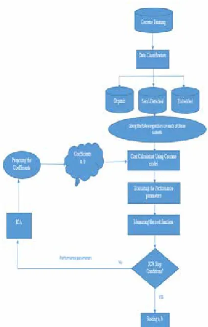
The flowchart of the proposed model is shown
in Figure 4. The experimental results show that
in contrast with COCOMO model, the MMRE is considerably decreased.
Figure 4: Flowchart of the proposed model
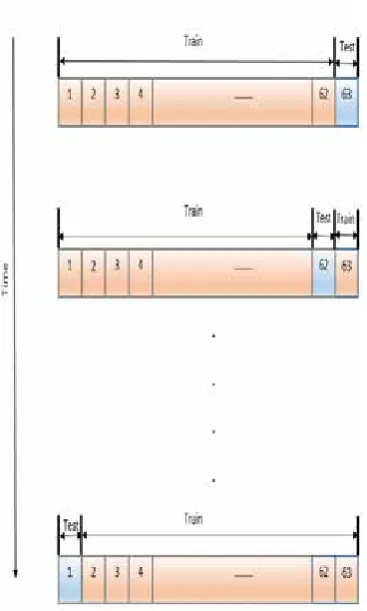
4. Leave one out cross validation (LOOCV) In LOOCV scenario, one of the observations is randomly selected as the test data and the rest of the observations are considered as train data. These data sets are given to the optimization algorithm. This process continues till all the observations are selected as test data. Here there are 63 records or observations. One of the records is selected as test data and the rest of records as train one and then the optimization process is performed on the train data. Then, this process is continued till all the records are selected as test data. At the end of this process, an array
with 63 members that are estimated efforts are
constructed. So it can be easy to compare the
results with the real efforts. This process always
has deterministic results although the only problem is that the training time of the algorithm in this form of cross validation is so long. A
Figure 5: A summary of applying Leave One Out Cross
Validation on COCOMO81 dataset
The pseudo code of the procedure is as follows:
for k =1 : sizeof(COCOMO81,1)
train_data and test_data sets are selected using LOOCV
Problem Statement
Algorithmic Parameter Setting Creation of Initial Empires Main Loop
Assimilation Revolution
New Cost Evaluation Empire Possession
Computation of Total Cost for Empires [MMRE]=Mycost(x, train_data)//Cost function call
[MMRE]=Mytest(a,b,test_data)//Test function Call
End
Where a and b are the two optimization variables.
V. Experimental Results
In order to measure the estimation accuracy of the ICA model, COCOMO dataset consisting of
63 records of real world software projects is used.
The simulation of the proposed model is done in the simulated environment of MATLAB 2014a. To evaluate the proposed model, the initial values of ICA parameters have been given values shown in Table 3. Number of initial countries is set to 180, empires number to 18, and also the parameter
decades which is equal to the maximum iteration
parameter in Genetic algorithm is set to 100. The lower bound and upper bound of the optimization variables are set to [-10, +10] interval. Parameter
β gets the value of 2. Increasing the value of the parameter γ increases the search of imperialist
environs and its decrease causes colonial move as much as possible, closer to the vector of connected colonials to colonies. The parameter zeta, which is a percentage of average cost of whole of the colonies in an imperialist, is set to 0.03. The training and testing processes were completed using leave one out cross validation.
Table 3- ICA parameters initialization.
Parameters values
No. Population 180
No. Imperials 18
No. Decades (Iterations) 100
Revolution rate 0.3
Varmin -10
Varmax +10
β 2
γ Π/4
Zeta 0.03
Training LOOCV
Testing LOOCV
In this experimental study, the process of evaluating the accuracy of SCE is done in three
experiences in which of them different data
orders are used.
1. Original COCOMO81
In the first experience, the ICA was trained
with the original COCOMO dataset without any changes using leave one out cross validation which is here called original COCOMO. In the proposed model, MMRE considered as the output
of the fitness function so that the objective of the fitness function is to minimize the amount of MMRE Eq. (12), Eq. (13), Eq. (14) and Eq. (15).
and PRED is about 0.3651 .Eq. (15).
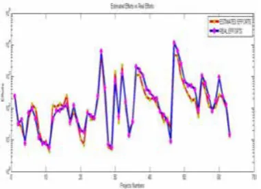
The plot diagram of estimated and real efforts in this experience is shown in figure 6. As it is
clear, the estimated values are very close to the real ones.
Figure 6: Effort estimation using original COCOMO dataset.
2. Separated COCOMO81
As it has been mentioned before, the
projects in COCOMO dataset are divided into
three categories: organic, semi-detached and embedded. In the second experience, the COCOMO dataset has been divided into these three separated datasets, and for each of these datasets, the ICA was separately trained using leave one out cross validation and then test it with the test data. There are three sets of results obtained from each run that are presented in
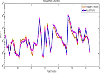
figures 8,9 and 10, but the final results, which can be seen in figure 7 are the mean of these three results and show that the best MRE is equal to
0.2702 while the MMRE is bout 0.3370 and the PRED value is 0.3571.
Figure 7: Real Efforts vs Estimated Efforts on Separated
COCOMO datasets.
In figure 8, the comparison of estimated efforts and real efforts on the organic dataset is
presented.
Figure 8: Real Efforts vs Estimated Efforts on organic dataset
In figure 9, the comparison of estimated efforts and real efforts on the semi-detached dataset is
presented either.
Figure 9: Real Efforts vs Estimated Efforts on semi-detached
dataset
In figure 10, the comparison of estimated efforts and real efforts on the embedded dataset
is presented.
Figure 10: Real Efforts vs Estimated Efforts on embedded
3. Ordered COCOMO81
And finally, in the third experience, the order
of COCOMO dataset values has been changed, in
such a way that all the organic projects come first and then the semi-detached projects are stored and finally all the embedded projects are placed. The difference between second experience
and third one, which is now called ordered COCOMO, is that in the second experience, for
each kind of projects, organic, semi-detached
and embedded, the ICA ran separately but in the
last experience, ICA ran just for one time on the ordered COCOMO dataset. Here just like the
previous experiences, at the beginning of the process, the ICA was trained using leave one out cross validation on the ordered COCOMO dataset and then it was tested with the test data. The results show that, the best MRE is about 0.3621and MMRE is about 0.3941 and PRED is about 0.3492. See Figure 11.
Figure 11: Real Efforts vs Estimated Efforts on the ordered
COCOMO dataset
In figure 12 the results of all the projects experiences has been presented in one figure and
also the result summary is shown in table 4 and table 5.
Figure 12: Estimated Efforts vs Real Efforts of all the
experiences
A brief summary of applying ICA on different
COCOMO datasets is shown in table4 and table5.
Table 4: The results of applying ICA on different COCOMO
datasets
Criterion Original cocomo Separated cocomo Ordered cocomo a and b 2.79 1.08 4.2283 0.9955 2.7665 1.0909
Best
MRE 0.3606 0.2702 0.3621
Table 5: Comparison of MMRE and PRED values of
applying ICA on different Cocomo datasets.
Criterion Original
cocomo Separated cocomo Ordered cocomo COCOMO81 MMRE 0.3903 0.2863 0.3941 0.3180 PRED 0.3651 0.3571 0.3492 0.3492
VI. Conclusion
In this paper, the ICA optimization strategy
was employed to estimate the effort based on
COCOMO81. ICA has been known as a very fast
and flexible strategy and could properly estimate the effort values. The proposed model was
REFERENCES
[1] Wold, Svante, et al. (1984). The Collinearity
Problem in Linear Regression. The Partial Least Squares
(PLS) Approach to Generalized Inverses, SIAM Journal on
Scientific and Statistical Computing, 5.6: 735-743.
[2] El, E. K, Gunes, A. k. (2008). A replicated survey of
IT software project failures. Software, IEEE 25.5: 84-90.
[3] Jorgensen, M., and MOLØKKEN-ØSTVOLD,
K.(2003). A review of surveys on software effort estimation.
International Symposium on Empirical Software Engineering (ISESE’03), Rome. Proceedings. IEEE Computer Society.
[4] Heiat, A. (2002). Comparison of artificial neural
network and regression models for estimating software
development effort. Information and software Technology
44.15: 911-922.
[5] Gharehchopogh, Soleimanian, F; et al. (2014). A Novel PSO based Approach with Hybrid of Fuzzy C-Means and Learning Automata in Software Cost Estimation. Indian Journal of Science and Technology 7.6: 795-803.
[6] Maleki, I. Gharehchopogh, Ayat, F. S, Ebrahimi, L. (2014). A Novel Hybrid Model of Scatter Search and Genetic Algorithms for Software Cost Estimation. MAGNT Research Report, 2 (6): 359-371.
[7] Leung, Hareton, Zhang, F. (2002). “Software cost estimation.” Handbook of Software Engineering, Hong Kong Polytechnic University.
[8] Gharehchopogh, Soleimanian, F; et al. (2014). A
Novel Hybrid Artificial Immune System with Genetic
Algorithm for Software Cost Estimation. MAGNT Research Report, 2 (6): 506-517.
[9] Atashpaz, G. E. et al. (2008).Colonial competitive algorithm: a novel approach for PID controller design in MIMO distillation column process. International Journal of Intelligent Computing and Cybernetics 1.3: 337-355.
[10] Boehm, B. W. (1981). Software engineering
economics. Englewood Cliffs, NJ: Prentice Hall.
[11] Hari, C. H., and Reddy, P. V. G. D. (2011). A
Fine Parameter Tuning for COCOMO 81 Software Effort
Estimation using Particle Swarm Optimization. Journal of Software Engineering 5.1.
[12] Catal, C., Mehmet, S. A. (2011). A Composite
Project Effort Estimation Approach in an Enterprise Software Development Project. SEKE.
[13] Bardsiri, V. k; et al. (2013). A PSO-based model
to increase the accuracy of software development effort
estimation. Software Quality Journal 21.3: 501-526. [14] Maroufi, Awat, Ahmad, J.(2015). ANew Approach
in Software Cost Estimation with Hybrid Imperialist Competitive Algorithm and Mamdani Fuzzy Model.