Classifier Ensemble Framework: a Diversity
Based Approach
Hamid Parvin1, Hosein Alizadeh2, Mohsen Moshki3
Received (2015-10-15) Accepted (2016-02-11)
Abstract—Pattern recognition systems are
widely used in a host of different fields. Due to some reasons such as lack of knowledge about a method based on which the best classifier is detected for any arbitrary problem, and thanks to significant improvement in accuracy, researchers turn to ensemble methods in almost every task of pattern recognition. Classification as a major task in pattern recognition, have been subject to this transition. The classifier ensemble which uses a number of base classifiers is considered as meta-classifier to learn any classification problem in pattern recognition. Although some researchers think they are better than single classifiers, they will not be better if some conditions are not met. The most important condition among them is diversity of base classifiers. Generally in design of multiple classifier systems, the more diverse the results of the classifiers, the more appropriate the aggregated result. It has been shown that the necessary diversity for the ensemble can be achieved by manipulation of dataset features, manipulation of data points in dataset, different sub-samplings of dataset, and usage of different classification algorithms. We also propose a new method of creating this diversity. We use Linear Discriminant Analysis to manipulate the data points in dataset. Although the classifier ensemble produced by proposed method may not always outperform all of its base classifiers, it always possesses the diversity needed for creation of an ensemble, and consequently it always outperforms all of its base classifiers on average.
Index Terms— Classifier Ensemble, Diversity,
Linear Discriminant Analysis.
I. INTRODUCTION
D
ifferent pattern recognition tasks are employed in different problems. Patternrecognition is considered as a general tool for
solving any problem in any field [2], [18-19], [21], [27-35]. Clearly, it is always needed to find a better pattern recognition model. Classification as a major task in pattern recognition is not an exception to this subject. Classification is a task that tries to predict category of some objects. In ensemble method for classification, many classifiers are combined to make a final prediction. Ensemble methods show better performances than a single classifier in general. The final decision is usually made by voting after combining the predictions from set of classifiers.
Most of the classification researches resulted
in algorithms that have provided a good
performance for specific problem, but they have not enough robustness for other problems. Because of the difficulty that these algorithms are faced to, the recent researches have been directed to the combinational methods that have more power, robustness, resistance, accuracy and generality [15]. Although the accuracy of the classifier ensemble is not always better than the most accurate classifier in ensemble pool, its
accuracy is never less than their average accuracy
[9]. Classifier ensemble can be considered as a
general solution method for pattern recognition
problems [14-15]. Inputs of classifier ensemble are predicted class tags of base classifiers and
its output is consensus predicted class tags. It is
an accepted subject in pattern recognition that finding the best classifier model for solving a given problem is impossible [22-23] and it has some serious drawbacks. The main drawback is
that the best individual classifier for the given classification problem is very difficult to identify, unless deep prior knowledge is available for such a task [3]. It is worthy to noting that the motivations in favor of classifier ensemble strongly resemble those of a “hybrid” intelligent system. The obvious reason for this is that classifier ensemble can be regarded as a special-purpose hybrid intelligent system.
It is believed that “combining the diverse classifiers any of which has better results than random ones, creates a good ensemble”. Diversity is always considered as a crucial concept in classifier ensemble. It is considered as the most effective factor in succeeding an ensemble. The diversity in an ensemble refers to the amount of
dissimilarity in the outputs of its components
(base classifiers) in deciding for a given sample. Assume an example dataset with two classes. Indeed the diversity concept for an ensemble of two classifiers refers to the probability that they may produce two dissimilar results for an arbitrary input sample. The diversity concept for an ensemble of three classifiers refers to the probability that one of them produces dissimilar result from the two others for an arbitrary input sample. It is worthy to mention that the diversity can converge to 0.5 and 0.66 in the ensembles of two and three classifiers respectively. Although reaching the more diverse ensemble of classifiers is generally handful, it is harmful in boundary limit. It is very important dilemma in classifier ensemble field: the ensemble of accurate/diverse classifiers can be the best. It means that although the more diverse classifiers, the better ensemble, it is provided that the classifiers are better than
random.
Classifier ensemble systems can be categorized by the ways they are built. Four dimensions for characterizing ensemble methods have been proposed: combination level, classifier level, feature level, and data level. In this article, we will focus on the classifier level and feature level that deals with the ways the base classifier are created and some new features may be created.
Bagging [1], Random Forest [5] and AdaBoost [6-8] may be the three most widely
used techniques to generate homogeneous
classifiers. Bagging trains its diverse classifiers by employing a primary learning algorithm to some bootstrapped samples. These
sub-samples are randomly extracted out of the train
dataset with replacement and have the same
sample size as that of the train dataset. Random
Forest [5] is an ensemble approach that uses a decision tree as its primary classifier. It uses bootstrapped sub-sampling to obtain different train datasets like Bagging. Both Bagging and Random Forest utilize simple majority voting mechanism to aggregate their primary classifiers into a consensus classifier. AdaBoost, the most prominent member in boosting family, generates a series of base classifiers by applying a given base learning algorithm to successive derived training sets that are obtained by either resampling or reweighting the original train dataset in the light of a weight distribution maintained over
the training set. AdaBoost initially assigns
equal weights to each training instance and in subsequent iterations, it adjusts these weights so that the weight of the instances misclassified by the previously trained classifier is increased, whereas that of the correctly predicted ones is
decreased. Thus, AdaBoost attempts to produce
new classifiers that are able to better predict the “hard” instances for the previous ensemble members. The final classification is obtained from a weighted vote of the base classifiers.
II. BACKGROUND
A classifier ensemble will be named a generative classifier ensemble if it produces base classifiers during the training of ensemble. In generative classifier ensemble methods, diversity is usually made using two categories of classifier ensembles. One category of these methods obtains diverse individuals by training classifiers on different training set, such as bagging [1], boosting [25], cross validation [20] and using artificial training examples [13]. Another category
of methods for creating diversity employs
different structures, different initial weighing, different parameters and different base classifiers to obtain ensemble individuals. For example, [24] adapted the training algorithm of the network by introducing a penalty term to encourage individual networks to be decorrelated. Liu and Yao [12] used negative correlation learning to
generate negatively correlated individual neural
network.
where the diverse components are selected from a number of trained accurate base classifiers. For example, Opitz and Shavlik [17] proposed
a generic algorithm to search for a highly
diverse set of accurate networks. Lazarevic and Obradoric [11] proposed a pruning algorithm to eliminate redundant classifiers. Navone et al. [16] proposed another selective algorithm based on bias/variance decomposition. GASEN proposed by Zhou et al. [26] and PSO based approach proposed by Fu et al. [4] also were introduced to select the ensemble components.
Linear Discriminant Analysis:
Linear discriminant analysis (LDA) is an
algorithm used in pattern recognition to discover
a linear transformation of attributes. It is widely
used to discover a linear mapping of dimensions
where data points of different classes in the
dataset are discriminated from each other. Indeed,
the objective function of LDA is to find the best locations for Gaussian distributions of different clusters and the best parameters for those Gaussian distributions in any given dataset. LDA tries to decrease dimensionality while preserving
as much of the class discriminatory information
as possible. The output of LDA can be considered as a linear classifier. It can also be considered as
dimensionality reduction technique.
However it is commonly considered as a dimensionality reduction. LDA is also closely
related to Principal Component Analysis (PCA)
in which it explores linear combinations of features which perfectly represent the data. As LDA is supervised, it tries to model the difference between the classes of data. PCA is an unsupervised task. So, PCA does not take into account any difference in class.
III. PROPOSED METHOD
Before presenting our method, some materials
must be clarified. Assume our dataset is always denoted by D. Our dataset contains n data points
and defined in a f-dimensional feature space. Also assume that our dataset has c classes. Let
us assume T is target vector. It means that Ti is category of ith data point. Also we assume that ith data point is denoted by Di.
Definition 1 data point: a vector of f
continuous values that represents a data object. So Dij is jth feature of ith data point.
Definition 2 hard classifier: a model that receives a data point and returns a categorical
label.
Definition 3 soft classifier: a model that receives a data point and returns a vector of c
continuous values where each value is in range [0,1]. The jth output of a soft classifier is denoted
by oj and represents for support of the classifier
for jth class. It means that when a data point is given to a soft classifier, it produces a vector 𝒐𝒐𝒐𝒐��⃗
that each value of that represents amount of
classifier support for its corresponding class for the data point. It is clear that if you are obliged to
select only one class tag for a data point using a soft classifier, the class with maximum support, is the best candidate. The class with maximum probability (definition 5) is named the most
probable tag (MPT). The class with the second maximum probability is named runner-up tag
(RUT).
Definition 4 support for a class: A value in range [0,1] produced by a soft classifier on a data point indicating how much the classifier believes
the data point belongs to that class.
Definition 5 probability for a class: A
probability value indicating the data point belongs to a class. To compute it, assume a soft
classifier output over a data point is a vector
𝒐𝒐𝒐𝒐��⃗= [𝑜𝑜𝑜𝑜1,𝑜𝑜𝑜𝑜2, …𝑜𝑜𝑜𝑜𝑐𝑐𝑐𝑐] . The probability vector is
𝒑𝒑𝒑𝒑��⃗ = [𝑝𝑝𝑝𝑝1, 𝑝𝑝𝑝𝑝2, … 𝑝𝑝𝑝𝑝𝑐𝑐𝑐𝑐] and computed based on
equation 1.
𝑝𝑝𝑝𝑝𝑖𝑖𝑖𝑖 =∑ �𝑃𝑃𝑃𝑃𝑃𝑃𝑃𝑃𝑖𝑖𝑖𝑖×𝑜𝑜𝑜𝑜𝑖𝑖𝑖𝑖 𝑗𝑗𝑗𝑗 ×𝑜𝑜𝑜𝑜𝑗𝑗𝑗𝑗� 𝑐𝑐𝑐𝑐
𝑗𝑗𝑗𝑗=1 (1)
where Pj is the prior probability presented in definition 11 and formulated in equation 2.
Definition 6ensemble support for a class: A value in range [0,1] produced by a soft classifier on a data point indicating how much the classifier believes the data point belongs to that class.
Definition 7 ensemble: a Ens_Size soft
classifiers that is denoted by E. It is worthy to
mention that Ei stands for ith soft classifier of the ensemble.
Definition 8ensemble support for a class: A value in range [0,1] produced by an ensemble
of soft classifiers on a data point indicating
belongs to that class. It is the averaged support
of soft classifiers on that data point for the class.
Definition 9 hard data point (HDP): A
data point will be defined as a hard data point
if (ensemble) probability difference between MPT and RUT is more than a threshold. The mentioned threshold that is denoted by hard_Th
is a parameter of the algorithm.
Definition 10erroneous data point (EDP): ith
data point will be defined as an erroneous data
point if MPT is not equal to Ti.
The proposed method gets dataset as input,
and puts it into three partitions: training set, test set and validation set. The size of training set
divided by the size of dataset is named training set ratio and denoted by TrR. The size of test set
divided by the size of dataset is named test set ratio and denoted by TeR. The size of validation set
divided by the size of dataset is named validation set ratio and denoted by VaR. Throughout the paper, training set, test set and validation set are
denoted by TrS, TeS and VaS respectively. Also in the paper, target vector of training set, test set and validation set are denoted by TTrS, TTeS and
TVaS respectively.
Definition 11 Prior Probability: a Pi where i{1,2,…,c} is computed based on equation 2.
𝑃𝑃𝑃𝑃𝑖𝑖𝑖𝑖 =𝑛𝑛𝑛𝑛𝑖𝑖𝑖𝑖 𝑇𝑇𝑇𝑇𝑇𝑇𝑇𝑇𝑇𝑇𝑇𝑇
𝑛𝑛𝑛𝑛𝑇𝑇𝑇𝑇𝑇𝑇𝑇𝑇𝑇𝑇𝑇𝑇 (2)
where niTrS is the number of data points of
class i in TrS and nTrS stands as the number of data points in TrS. The algorithm is depicted in Fig. 1.
Then the data of each class is extracted from the original validation data set. The proposed
algorithm assumes that a classifier is first trained on training set, and then this classifier is added to our ensemble. Now using this classifier, we can obtain erroneous data points on validation data set. Using this work we partition validation data points into two classes: erroneous and non-erroneous. At this step, we label validation data points according the two above classes and then using a pairwise classifier we approximate probability of the error occurrence. This pairwise classifier indeed works as an error detector. Next
all data, including training, testing and validation
are served as input for that classifier, and then their outputs are considered as new features of
those data points. At the next step, using linear
discriminant analysis (LDA) we reduce the dimensionality of the above new space to that of previous space [3]. We repeat this process in predefined number of iterations. Repeating the above process as many as the predefined number causes to creation of that predefined number of data sets and consequently also that number of classifiers.
---Inputs:
𝑇𝑇𝑇𝑇𝑇𝑇𝑇𝑇𝑇𝑇𝑇𝑇,𝑇𝑇𝑇𝑇𝑇𝑇𝑇𝑇𝑇𝑇𝑇𝑇,𝑉𝑉𝑉𝑉𝑉𝑉𝑉𝑉𝑇𝑇𝑇𝑇,𝐷𝐷𝐷𝐷,𝑐𝑐𝑐𝑐,𝐸𝐸𝐸𝐸𝐸𝐸𝐸𝐸𝐸𝐸𝐸𝐸_𝑆𝑆𝑆𝑆𝑆𝑆𝑆𝑆𝑆𝑆𝑆𝑆𝑇𝑇𝑇𝑇,𝐸𝐸𝐸𝐸𝑇𝑇𝑇𝑇𝑇𝑇𝑇𝑇𝐸𝐸𝐸𝐸𝐸𝐸𝐸𝐸𝑇𝑇𝑇𝑇𝐸𝐸𝐸𝐸𝐸𝐸𝐸𝐸𝐸𝐸𝐸𝐸_𝑇𝑇𝑇𝑇ℎ,𝑇𝑇𝑇𝑇, @𝑇𝑇𝑇𝑇𝑇𝑇𝑇𝑇𝑉𝑉𝑉𝑉𝑆𝑆𝑆𝑆𝐸𝐸𝐸𝐸𝑆𝑆𝑆𝑆𝐸𝐸𝐸𝐸𝑇𝑇𝑇𝑇𝑇𝑇𝑇𝑇𝑇𝑇𝑇𝑇𝑇𝑇𝑇𝑇𝑉𝑉𝑉𝑉𝐸𝐸𝐸𝐸𝐸𝐸𝐸𝐸𝑆𝑆𝑆𝑆𝑇𝑇𝑇𝑇𝑆𝑆𝑆𝑆𝑇𝑇𝑇𝑇𝑇𝑇𝑇𝑇
Output:
𝐸𝐸𝐸𝐸,𝐸𝐸𝐸𝐸𝑇𝑇𝑇𝑇𝑇𝑇𝑇𝑇𝐸𝐸𝐸𝐸𝑇𝑇𝑇𝑇
𝐵𝐵𝐵𝐵𝑇𝑇𝑇𝑇𝐵𝐵𝐵𝐵𝑆𝑆𝑆𝑆𝐸𝐸𝐸𝐸 𝐷𝐷𝐷𝐷=𝑆𝑆𝑆𝑆ℎ𝐸𝐸𝐸𝐸𝑇𝑇𝑇𝑇𝑇𝑇𝑇𝑇𝑇𝑇𝑇𝑇𝑇𝑇𝑇𝑇(𝐷𝐷𝐷𝐷)
𝑇𝑇𝑇𝑇𝑇𝑇𝑇𝑇𝑆𝑆𝑆𝑆=𝑇𝑇𝑇𝑇𝐸𝐸𝐸𝐸𝐸𝐸𝐸𝐸𝐸𝐸𝐸𝐸𝑟𝑟𝑟𝑟(𝐸𝐸𝐸𝐸×𝑇𝑇𝑇𝑇𝑇𝑇𝑇𝑇𝑇𝑇𝑇𝑇)
𝑇𝑇𝑇𝑇𝑇𝑇𝑇𝑇𝑆𝑆𝑆𝑆=𝑇𝑇𝑇𝑇𝐸𝐸𝐸𝐸𝐸𝐸𝐸𝐸𝐸𝐸𝐸𝐸𝑟𝑟𝑟𝑟(𝐸𝐸𝐸𝐸×𝑇𝑇𝑇𝑇𝑇𝑇𝑇𝑇𝑇𝑇𝑇𝑇)
𝑉𝑉𝑉𝑉𝑉𝑉𝑉𝑉𝑆𝑆𝑆𝑆 =𝑇𝑇𝑇𝑇𝐸𝐸𝐸𝐸𝐸𝐸𝐸𝐸𝐸𝐸𝐸𝐸𝑟𝑟𝑟𝑟(𝐸𝐸𝐸𝐸×𝑉𝑉𝑉𝑉𝑉𝑉𝑉𝑉𝑇𝑇𝑇𝑇)
𝑇𝑇𝑇𝑇𝑇𝑇𝑇𝑇𝐷𝐷𝐷𝐷=𝐷𝐷𝐷𝐷1..𝑇𝑇𝑇𝑇𝑇𝑇𝑇𝑇𝑆𝑆𝑆𝑆 𝑇𝑇𝑇𝑇𝑇𝑇𝑇𝑇𝑇𝑇𝑇𝑇𝐷𝐷𝐷𝐷=𝑇𝑇𝑇𝑇1..𝑇𝑇𝑇𝑇𝑇𝑇𝑇𝑇𝑆𝑆𝑆𝑆
𝑇𝑇𝑇𝑇𝑇𝑇𝑇𝑇𝐷𝐷𝐷𝐷=𝐷𝐷𝐷𝐷(𝑇𝑇𝑇𝑇𝑇𝑇𝑇𝑇𝑆𝑆𝑆𝑆+1)..(𝑇𝑇𝑇𝑇𝑇𝑇𝑇𝑇𝑆𝑆𝑆𝑆+𝑉𝑉𝑉𝑉𝑉𝑉𝑉𝑉𝑆𝑆𝑆𝑆) 𝑇𝑇𝑇𝑇𝑇𝑇𝑇𝑇𝑇𝑇𝑇𝑇𝐷𝐷𝐷𝐷=𝑇𝑇𝑇𝑇(𝑇𝑇𝑇𝑇𝑇𝑇𝑇𝑇𝑆𝑆𝑆𝑆+1)..(𝑇𝑇𝑇𝑇𝑇𝑇𝑇𝑇𝑆𝑆𝑆𝑆+𝑉𝑉𝑉𝑉𝑉𝑉𝑉𝑉𝑆𝑆𝑆𝑆) 𝑉𝑉𝑉𝑉𝑉𝑉𝑉𝑉𝐷𝐷𝐷𝐷=𝐷𝐷𝐷𝐷(𝑇𝑇𝑇𝑇𝑇𝑇𝑇𝑇𝑆𝑆𝑆𝑆+𝑉𝑉𝑉𝑉𝑉𝑉𝑉𝑉𝑆𝑆𝑆𝑆+1)..(𝑇𝑇𝑇𝑇𝑇𝑇𝑇𝑇𝑆𝑆𝑆𝑆+𝑉𝑉𝑉𝑉𝑉𝑉𝑉𝑉𝑆𝑆𝑆𝑆+𝑇𝑇𝑇𝑇𝑇𝑇𝑇𝑇𝑆𝑆𝑆𝑆)
𝑇𝑇𝑇𝑇𝑉𝑉𝑉𝑉𝑉𝑉𝑉𝑉𝐷𝐷𝐷𝐷=𝑇𝑇𝑇𝑇(𝑇𝑇𝑇𝑇𝑇𝑇𝑇𝑇𝑆𝑆𝑆𝑆+𝑉𝑉𝑉𝑉𝑉𝑉𝑉𝑉𝑆𝑆𝑆𝑆+1)..(𝑇𝑇𝑇𝑇𝑇𝑇𝑇𝑇𝑆𝑆𝑆𝑆+𝑉𝑉𝑉𝑉𝑉𝑉𝑉𝑉𝑆𝑆𝑆𝑆+𝑇𝑇𝑇𝑇𝑇𝑇𝑇𝑇𝑆𝑆𝑆𝑆) 𝐹𝐹𝐹𝐹𝐸𝐸𝐸𝐸𝑇𝑇𝑇𝑇𝑆𝑆𝑆𝑆= 1. .𝑐𝑐𝑐𝑐
𝑃𝑃𝑃𝑃𝑆𝑆𝑆𝑆=𝐸𝐸𝐸𝐸𝑆𝑆𝑆𝑆
𝑇𝑇𝑇𝑇𝑇𝑇𝑇𝑇𝑆𝑆𝑆𝑆
𝐸𝐸𝐸𝐸𝑇𝑇𝑇𝑇𝑇𝑇𝑇𝑇𝑆𝑆𝑆𝑆
𝐸𝐸𝐸𝐸𝐸𝐸𝐸𝐸𝑟𝑟𝑟𝑟
𝐸𝐸𝐸𝐸=∅
𝐹𝐹𝐹𝐹𝐸𝐸𝐸𝐸𝑇𝑇𝑇𝑇𝑆𝑆𝑆𝑆= 1 𝑇𝑇𝑇𝑇𝐸𝐸𝐸𝐸𝐸𝐸𝐸𝐸𝐸𝐸𝐸𝐸𝐸𝐸𝐸𝐸_𝑆𝑆𝑆𝑆𝑆𝑆𝑆𝑆𝑆𝑆𝑆𝑆𝑇𝑇𝑇𝑇
𝐸𝐸𝐸𝐸𝑆𝑆𝑆𝑆=𝑇𝑇𝑇𝑇𝑇𝑇𝑇𝑇𝑉𝑉𝑉𝑉𝑆𝑆𝑆𝑆𝐸𝐸𝐸𝐸𝑆𝑆𝑆𝑆𝐸𝐸𝐸𝐸𝑇𝑇𝑇𝑇𝑇𝑇𝑇𝑇𝑇𝑇𝑇𝑇𝑇𝑇𝑇𝑇𝑉𝑉𝑉𝑉𝐸𝐸𝐸𝐸𝐸𝐸𝐸𝐸𝑆𝑆𝑆𝑆𝑇𝑇𝑇𝑇𝑆𝑆𝑆𝑆𝑇𝑇𝑇𝑇𝑇𝑇𝑇𝑇(𝑇𝑇𝑇𝑇𝑇𝑇𝑇𝑇𝐷𝐷𝐷𝐷,𝑇𝑇𝑇𝑇𝑇𝑇𝑇𝑇𝑇𝑇𝑇𝑇𝐷𝐷𝐷𝐷) 𝐸𝐸𝐸𝐸𝐸𝐸𝐸𝐸𝑟𝑟𝑟𝑟
𝐻𝐻𝐻𝐻𝐷𝐷𝐷𝐷_𝐼𝐼𝐼𝐼𝐸𝐸𝐸𝐸𝑟𝑟𝑟𝑟=𝐻𝐻𝐻𝐻𝑉𝑉𝑉𝑉𝑇𝑇𝑇𝑇𝑟𝑟𝑟𝑟𝐷𝐷𝐷𝐷𝑉𝑉𝑉𝑉𝑇𝑇𝑇𝑇𝑉𝑉𝑉𝑉𝐷𝐷𝐷𝐷𝑇𝑇𝑇𝑇𝑇𝑇𝑇𝑇𝑇𝑇𝑇𝑇𝑐𝑐𝑐𝑐𝑇𝑇𝑇𝑇𝑆𝑆𝑆𝑆𝐸𝐸𝐸𝐸𝐸𝐸𝐸𝐸(𝐸𝐸𝐸𝐸,𝑃𝑃𝑃𝑃,𝐷𝐷𝐷𝐷,𝑇𝑇𝑇𝑇,𝐸𝐸𝐸𝐸𝑇𝑇𝑇𝑇𝑇𝑇𝑇𝑇𝐸𝐸𝐸𝐸𝐸𝐸𝐸𝐸𝑇𝑇𝑇𝑇𝐸𝐸𝐸𝐸𝐸𝐸𝐸𝐸𝐸𝐸𝐸𝐸_𝑇𝑇𝑇𝑇ℎ)
𝐸𝐸𝐸𝐸𝐷𝐷𝐷𝐷_𝐼𝐼𝐼𝐼𝐸𝐸𝐸𝐸𝑟𝑟𝑟𝑟=𝐸𝐸𝐸𝐸𝑇𝑇𝑇𝑇𝑇𝑇𝑇𝑇𝐸𝐸𝐸𝐸𝐸𝐸𝐸𝐸𝑇𝑇𝑇𝑇𝐸𝐸𝐸𝐸𝐸𝐸𝐸𝐸𝐸𝐸𝐸𝐸𝐷𝐷𝐷𝐷𝑉𝑉𝑉𝑉𝑇𝑇𝑇𝑇𝑉𝑉𝑉𝑉𝐷𝐷𝐷𝐷𝑇𝑇𝑇𝑇𝑇𝑇𝑇𝑇𝑇𝑇𝑇𝑇𝑐𝑐𝑐𝑐𝑇𝑇𝑇𝑇𝑆𝑆𝑆𝑆𝐸𝐸𝐸𝐸𝐸𝐸𝐸𝐸(𝐸𝐸𝐸𝐸,𝑃𝑃𝑃𝑃,𝐷𝐷𝐷𝐷,𝑇𝑇𝑇𝑇)
𝐻𝐻𝐻𝐻𝐷𝐷𝐷𝐷𝑇𝑇𝑇𝑇𝑆𝑆𝑆𝑆=�01 𝑆𝑆𝑆𝑆 ∈ 𝐻𝐻𝐻𝐻𝐷𝐷𝐷𝐷𝐸𝐸𝐸𝐸𝑇𝑇𝑇𝑇ℎ𝑇𝑇𝑇𝑇𝑇𝑇𝑇𝑇𝑒𝑒𝑒𝑒𝑆𝑆𝑆𝑆𝐸𝐸𝐸𝐸𝑇𝑇𝑇𝑇_𝐼𝐼𝐼𝐼𝐸𝐸𝐸𝐸𝑟𝑟𝑟𝑟,𝑒𝑒𝑒𝑒ℎ𝑇𝑇𝑇𝑇𝑇𝑇𝑇𝑇𝑇𝑇𝑇𝑇𝑆𝑆𝑆𝑆 ∈{1. . (𝑇𝑇𝑇𝑇𝑇𝑇𝑇𝑇𝑆𝑆𝑆𝑆+𝑉𝑉𝑉𝑉𝑉𝑉𝑉𝑉𝑆𝑆𝑆𝑆)} 𝐸𝐸𝐸𝐸𝐷𝐷𝐷𝐷𝑇𝑇𝑇𝑇𝑆𝑆𝑆𝑆=�01 𝑆𝑆𝑆𝑆 ∈ 𝐸𝐸𝐸𝐸𝐷𝐷𝐷𝐷𝐸𝐸𝐸𝐸𝑇𝑇𝑇𝑇ℎ𝑇𝑇𝑇𝑇𝑇𝑇𝑇𝑇𝑒𝑒𝑒𝑒𝑆𝑆𝑆𝑆𝐸𝐸𝐸𝐸𝑇𝑇𝑇𝑇_𝐼𝐼𝐼𝐼𝐸𝐸𝐸𝐸𝑟𝑟𝑟𝑟,𝑒𝑒𝑒𝑒ℎ𝑇𝑇𝑇𝑇𝑇𝑇𝑇𝑇𝑇𝑇𝑇𝑇𝑆𝑆𝑆𝑆 ∈{1. . (𝑇𝑇𝑇𝑇𝑇𝑇𝑇𝑇𝑆𝑆𝑆𝑆+𝑉𝑉𝑉𝑉𝑉𝑉𝑉𝑉𝑆𝑆𝑆𝑆)} 𝐻𝐻𝐻𝐻𝐷𝐷𝐷𝐷𝑇𝑇𝑇𝑇𝑇𝑇𝑇𝑇𝑉𝑉𝑉𝑉𝐸𝐸𝐸𝐸𝐸𝐸𝐸𝐸𝑆𝑆𝑆𝑆𝑇𝑇𝑇𝑇𝑆𝑆𝑆𝑆𝑇𝑇𝑇𝑇𝑇𝑇𝑇𝑇=𝑇𝑇𝑇𝑇𝑇𝑇𝑇𝑇𝑉𝑉𝑉𝑉𝑆𝑆𝑆𝑆𝐸𝐸𝐸𝐸𝑆𝑆𝑆𝑆𝐸𝐸𝐸𝐸𝑇𝑇𝑇𝑇𝑇𝑇𝑇𝑇𝑇𝑇𝑇𝑇𝑇𝑇𝑇𝑇𝑉𝑉𝑉𝑉𝐸𝐸𝐸𝐸𝐸𝐸𝐸𝐸𝑆𝑆𝑆𝑆𝑇𝑇𝑇𝑇𝑆𝑆𝑆𝑆𝑇𝑇𝑇𝑇𝑇𝑇𝑇𝑇�𝐷𝐷𝐷𝐷1..(𝑇𝑇𝑇𝑇𝑇𝑇𝑇𝑇𝑆𝑆𝑆𝑆+𝑉𝑉𝑉𝑉𝑉𝑉𝑉𝑉𝑆𝑆𝑆𝑆),𝐻𝐻𝐻𝐻𝐷𝐷𝐷𝐷𝑇𝑇𝑇𝑇� 𝐸𝐸𝐸𝐸𝐷𝐷𝐷𝐷𝑇𝑇𝑇𝑇𝑇𝑇𝑇𝑇𝑉𝑉𝑉𝑉𝐸𝐸𝐸𝐸𝐸𝐸𝐸𝐸𝑆𝑆𝑆𝑆𝑇𝑇𝑇𝑇𝑆𝑆𝑆𝑆𝑇𝑇𝑇𝑇𝑇𝑇𝑇𝑇=𝑇𝑇𝑇𝑇𝑇𝑇𝑇𝑇𝑉𝑉𝑉𝑉𝑆𝑆𝑆𝑆𝐸𝐸𝐸𝐸𝑆𝑆𝑆𝑆𝐸𝐸𝐸𝐸𝑇𝑇𝑇𝑇𝑇𝑇𝑇𝑇𝑇𝑇𝑇𝑇𝑇𝑇𝑇𝑇𝑉𝑉𝑉𝑉𝐸𝐸𝐸𝐸𝐸𝐸𝐸𝐸𝑆𝑆𝑆𝑆𝑇𝑇𝑇𝑇𝑆𝑆𝑆𝑆𝑇𝑇𝑇𝑇𝑇𝑇𝑇𝑇�𝐷𝐷𝐷𝐷1..(𝑇𝑇𝑇𝑇𝑇𝑇𝑇𝑇𝑆𝑆𝑆𝑆+𝑉𝑉𝑉𝑉𝑉𝑉𝑉𝑉𝑆𝑆𝑆𝑆),𝐸𝐸𝐸𝐸𝐷𝐷𝐷𝐷𝑇𝑇𝑇𝑇� 𝑇𝑇𝑇𝑇𝑇𝑇𝑇𝑇𝐸𝐸𝐸𝐸𝑇𝑇𝑇𝑇𝐻𝐻𝐻𝐻𝐷𝐷𝐷𝐷𝑃𝑃𝑃𝑃𝑇𝑇𝑇𝑇𝑇𝑇𝑇𝑇𝑟𝑟𝑟𝑟𝑆𝑆𝑆𝑆𝑐𝑐𝑐𝑐𝑇𝑇𝑇𝑇=𝑇𝑇𝑇𝑇𝑇𝑇𝑇𝑇𝐸𝐸𝐸𝐸𝑇𝑇𝑇𝑇(𝐻𝐻𝐻𝐻𝐷𝐷𝐷𝐷𝑇𝑇𝑇𝑇𝑇𝑇𝑇𝑇𝑉𝑉𝑉𝑉𝐸𝐸𝐸𝐸𝐸𝐸𝐸𝐸𝑆𝑆𝑆𝑆𝑇𝑇𝑇𝑇𝑆𝑆𝑆𝑆𝑇𝑇𝑇𝑇𝑇𝑇𝑇𝑇,𝑇𝑇𝑇𝑇𝑇𝑇𝑇𝑇𝐷𝐷𝐷𝐷)
𝑇𝑇𝑇𝑇𝑇𝑇𝑇𝑇𝐸𝐸𝐸𝐸𝑇𝑇𝑇𝑇𝐸𝐸𝐸𝐸𝐷𝐷𝐷𝐷𝑃𝑃𝑃𝑃𝑇𝑇𝑇𝑇𝑇𝑇𝑇𝑇𝑟𝑟𝑟𝑟𝑆𝑆𝑆𝑆𝑐𝑐𝑐𝑐𝑇𝑇𝑇𝑇=𝑇𝑇𝑇𝑇𝑇𝑇𝑇𝑇𝐸𝐸𝐸𝐸𝑇𝑇𝑇𝑇(𝐸𝐸𝐸𝐸𝐷𝐷𝐷𝐷𝑇𝑇𝑇𝑇𝑇𝑇𝑇𝑇𝑉𝑉𝑉𝑉𝐸𝐸𝐸𝐸𝐸𝐸𝐸𝐸𝑆𝑆𝑆𝑆𝑇𝑇𝑇𝑇𝑆𝑆𝑆𝑆𝑇𝑇𝑇𝑇𝑇𝑇𝑇𝑇,𝑇𝑇𝑇𝑇𝑇𝑇𝑇𝑇𝐷𝐷𝐷𝐷)
𝑁𝑁𝑁𝑁𝑇𝑇𝑇𝑇𝑒𝑒𝑒𝑒𝐷𝐷𝐷𝐷=𝐷𝐷𝐷𝐷
𝑁𝑁𝑁𝑁𝑇𝑇𝑇𝑇𝑒𝑒𝑒𝑒𝐷𝐷𝐷𝐷𝑆𝑆𝑆𝑆,(𝑇𝑇𝑇𝑇+1)=𝐻𝐻𝐻𝐻𝐷𝐷𝐷𝐷𝑇𝑇𝑇𝑇𝑆𝑆𝑆𝑆 ,𝑒𝑒𝑒𝑒ℎ𝑇𝑇𝑇𝑇𝑇𝑇𝑇𝑇𝑇𝑇𝑇𝑇𝑆𝑆𝑆𝑆 ∈{1. . (𝑇𝑇𝑇𝑇𝑇𝑇𝑇𝑇𝑆𝑆𝑆𝑆+𝑉𝑉𝑉𝑉𝑉𝑉𝑉𝑉𝑆𝑆𝑆𝑆)}
𝑁𝑁𝑁𝑁𝑇𝑇𝑇𝑇𝑒𝑒𝑒𝑒𝐷𝐷𝐷𝐷(𝑇𝑇𝑇𝑇𝑇𝑇𝑇𝑇𝑆𝑆𝑆𝑆+𝑉𝑉𝑉𝑉𝑉𝑉𝑉𝑉𝑆𝑆𝑆𝑆)+𝑆𝑆𝑆𝑆,(𝑇𝑇𝑇𝑇+1)=𝐻𝐻𝐻𝐻𝐷𝐷𝐷𝐷𝑇𝑇𝑇𝑇𝑇𝑇𝑇𝑇𝑉𝑉𝑉𝑉𝐸𝐸𝐸𝐸𝐸𝐸𝐸𝐸𝑆𝑆𝑆𝑆𝑇𝑇𝑇𝑇𝑆𝑆𝑆𝑆𝑇𝑇𝑇𝑇𝑇𝑇𝑇𝑇𝑆𝑆𝑆𝑆 ,𝑒𝑒𝑒𝑒ℎ𝑇𝑇𝑇𝑇𝑇𝑇𝑇𝑇𝑇𝑇𝑇𝑇𝑆𝑆𝑆𝑆 ∈{1, . . ,𝑇𝑇𝑇𝑇𝑇𝑇𝑇𝑇𝑆𝑆𝑆𝑆} 𝑁𝑁𝑁𝑁𝑇𝑇𝑇𝑇𝑒𝑒𝑒𝑒𝐷𝐷𝐷𝐷𝑆𝑆𝑆𝑆,(𝑇𝑇𝑇𝑇+2)=𝐸𝐸𝐸𝐸𝐷𝐷𝐷𝐷𝑇𝑇𝑇𝑇𝑆𝑆𝑆𝑆 ,𝑒𝑒𝑒𝑒ℎ𝑇𝑇𝑇𝑇𝑇𝑇𝑇𝑇𝑇𝑇𝑇𝑇𝑆𝑆𝑆𝑆 ∈{1. . (𝑇𝑇𝑇𝑇𝑇𝑇𝑇𝑇𝑆𝑆𝑆𝑆+𝑉𝑉𝑉𝑉𝑉𝑉𝑉𝑉𝑆𝑆𝑆𝑆)}
𝑁𝑁𝑁𝑁𝑇𝑇𝑇𝑇𝑒𝑒𝑒𝑒𝐷𝐷𝐷𝐷(𝑇𝑇𝑇𝑇𝑇𝑇𝑇𝑇𝑆𝑆𝑆𝑆+𝑉𝑉𝑉𝑉𝑉𝑉𝑉𝑉𝑆𝑆𝑆𝑆)+𝑆𝑆𝑆𝑆,(𝑇𝑇𝑇𝑇+1)=𝐸𝐸𝐸𝐸𝐷𝐷𝐷𝐷𝑇𝑇𝑇𝑇𝑇𝑇𝑇𝑇𝑉𝑉𝑉𝑉𝐸𝐸𝐸𝐸𝐸𝐸𝐸𝐸𝑆𝑆𝑆𝑆𝑇𝑇𝑇𝑇𝑆𝑆𝑆𝑆𝑇𝑇𝑇𝑇𝑇𝑇𝑇𝑇𝑆𝑆𝑆𝑆 ,𝑒𝑒𝑒𝑒ℎ𝑇𝑇𝑇𝑇𝑇𝑇𝑇𝑇𝑇𝑇𝑇𝑇𝑆𝑆𝑆𝑆 ∈{1, . . ,𝑇𝑇𝑇𝑇𝑇𝑇𝑇𝑇𝑆𝑆𝑆𝑆} 𝑇𝑇𝑇𝑇𝑇𝑇𝑇𝑇𝐷𝐷𝐷𝐷=𝑁𝑁𝑁𝑁𝑇𝑇𝑇𝑇𝑒𝑒𝑒𝑒𝐷𝐷𝐷𝐷1..𝑇𝑇𝑇𝑇𝑇𝑇𝑇𝑇𝑆𝑆𝑆𝑆
𝑇𝑇𝑇𝑇𝑇𝑇𝑇𝑇𝐷𝐷𝐷𝐷=𝑁𝑁𝑁𝑁𝑇𝑇𝑇𝑇𝑒𝑒𝑒𝑒𝐷𝐷𝐷𝐷(𝑇𝑇𝑇𝑇𝑇𝑇𝑇𝑇𝑆𝑆𝑆𝑆+1)..(𝑇𝑇𝑇𝑇𝑇𝑇𝑇𝑇𝑆𝑆𝑆𝑆+𝑉𝑉𝑉𝑉𝑉𝑉𝑉𝑉𝑆𝑆𝑆𝑆) 𝑉𝑉𝑉𝑉𝑉𝑉𝑉𝑉𝐷𝐷𝐷𝐷=𝑁𝑁𝑁𝑁𝑇𝑇𝑇𝑇𝑒𝑒𝑒𝑒𝐷𝐷𝐷𝐷(𝑇𝑇𝑇𝑇𝑇𝑇𝑇𝑇𝑆𝑆𝑆𝑆+𝑉𝑉𝑉𝑉𝑉𝑉𝑉𝑉𝑆𝑆𝑆𝑆+1)..(𝑇𝑇𝑇𝑇𝑇𝑇𝑇𝑇𝑆𝑆𝑆𝑆+𝑉𝑉𝑉𝑉𝑉𝑉𝑉𝑉𝑆𝑆𝑆𝑆+𝑇𝑇𝑇𝑇𝑇𝑇𝑇𝑇𝑆𝑆𝑆𝑆) 𝐹𝐹𝐹𝐹𝐸𝐸𝐸𝐸𝑇𝑇𝑇𝑇𝑆𝑆𝑆𝑆= 1 𝑇𝑇𝑇𝑇𝐸𝐸𝐸𝐸𝐸𝐸𝐸𝐸𝐸𝐸𝐸𝐸𝐸𝐸𝐸𝐸_𝑆𝑆𝑆𝑆𝑆𝑆𝑆𝑆𝑆𝑆𝑆𝑆𝑇𝑇𝑇𝑇
𝐸𝐸𝐸𝐸𝑆𝑆𝑆𝑆=𝑇𝑇𝑇𝑇𝑇𝑇𝑇𝑇𝑉𝑉𝑉𝑉𝑆𝑆𝑆𝑆𝐸𝐸𝐸𝐸𝑆𝑆𝑆𝑆𝐸𝐸𝐸𝐸𝑇𝑇𝑇𝑇𝑇𝑇𝑇𝑇𝑇𝑇𝑇𝑇𝑇𝑇𝑇𝑇𝑉𝑉𝑉𝑉𝐸𝐸𝐸𝐸𝐸𝐸𝐸𝐸𝑆𝑆𝑆𝑆𝑇𝑇𝑇𝑇𝑆𝑆𝑆𝑆𝑇𝑇𝑇𝑇𝑇𝑇𝑇𝑇(𝑇𝑇𝑇𝑇𝑇𝑇𝑇𝑇𝐷𝐷𝐷𝐷,𝑇𝑇𝑇𝑇𝑇𝑇𝑇𝑇𝑇𝑇𝑇𝑇𝐷𝐷𝐷𝐷) 𝐸𝐸𝐸𝐸𝐸𝐸𝐸𝐸𝑟𝑟𝑟𝑟
𝐸𝐸𝐸𝐸𝐷𝐷𝐷𝐷_𝐼𝐼𝐼𝐼𝐸𝐸𝐸𝐸𝑟𝑟𝑟𝑟=𝐸𝐸𝐸𝐸𝑇𝑇𝑇𝑇𝑇𝑇𝑇𝑇𝐸𝐸𝐸𝐸𝐸𝐸𝐸𝐸𝑇𝑇𝑇𝑇𝐸𝐸𝐸𝐸𝐸𝐸𝐸𝐸𝐸𝐸𝐸𝐸𝐷𝐷𝐷𝐷𝑉𝑉𝑉𝑉𝑇𝑇𝑇𝑇𝑉𝑉𝑉𝑉𝐷𝐷𝐷𝐷𝑇𝑇𝑇𝑇𝑇𝑇𝑇𝑇𝑇𝑇𝑇𝑇𝑐𝑐𝑐𝑐𝑇𝑇𝑇𝑇𝑆𝑆𝑆𝑆𝐸𝐸𝐸𝐸𝐸𝐸𝐸𝐸(𝐸𝐸𝐸𝐸,𝑃𝑃𝑃𝑃,𝑁𝑁𝑁𝑁𝑇𝑇𝑇𝑇𝑒𝑒𝑒𝑒𝐷𝐷𝐷𝐷,𝑇𝑇𝑇𝑇)
𝐸𝐸𝐸𝐸𝑇𝑇𝑇𝑇𝑇𝑇𝑇𝑇𝐸𝐸𝐸𝐸𝑇𝑇𝑇𝑇=|𝐸𝐸𝐸𝐸𝐷𝐷𝐷𝐷_𝐸𝐸𝐸𝐸𝐼𝐼𝐼𝐼𝐸𝐸𝐸𝐸𝑟𝑟𝑟𝑟|
---Fig. 1. The pseudo code of the proposed combinational algorithm
Pseudo code of the proposed algorithm is
shown in Fig. 1. It can be said about time order
of this algorithm that the method just multiplies a constant multiplicand in the time order of simple
number). Then the time order of this method is Ω(3*m*f(n,c)). Consequently the time order of the method will be Ω(m*f(n,c)). This shows time
order of the algorithm relevant to just a constant
factor is reduced, that this waste of time is completely tolerable against important achieved
accuracy.
After creating diverse classifiers for our classifier ensemble, the next step is finding a method to fuse their results and make final decision. The part of making final decision is named combiner part. There are many different combiners. Combination method of base classifier decisions depend on their output type. Some traditional methods of classifier fusion which are based on soft/fuzzy outputs are as below:
Majority vote: assume that we have k classifiers. Classifier ensemble vote to class j if a little more than half of base classifiers vote to
class j.
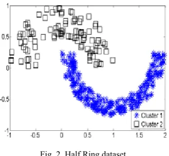
Fig. 2. Half Ring dataset.
Simple average: the average of results of separate classifiers is calculated and then the
class that has the most average value is selected
as final decision.
Weighted average: it is like simple average except that a weight for each classifier is used for
calculating that average.
IV. EXPRIMENTAL RESULTS
The metric for evaluating an output of a
classifier is accuracy; i.e.the accuracy is taken as
the evaluation metric throughout all the paper for
reporting performance of classifiers.
The proposed method is examined over 6
different standard datasets and one artificial dataset. These real datasets are available at UCI repository [11]. Brief information about the used datasets is available in Table 1. The details of
HalfRing dataset can be available in [14]. The artificial HalfRing dataset is depicted in Fig. 2.
The HalfRing dataset is considered as one of the
most challenging dataset for the classification
algorithms.
Table 1. Brief information about the used datasets.
# Dataset Name Class# of Features# of Samples# of Data distribution per classes
1 Halfrings 2 2 400 300-100 2 Ionosphere 2 34 351 126-225 3 Iris 3 4 150 50-50-50
4 Wine 3 13 178 59-71-48
5 Bupa 2 6 345 145-200 6 BreastCancer 683 9 2 444-239 7 Yeast 1484 8 10 463-5-35-44
-51-163-244-429 -20-30
The predefined number of max_iteration in
the algorithm is experimentally considered 3 here. Here, train set, test set and validation set are considered to contain 60%, 15% and 25% of entire dataset respectively. The summery of
the results are reported in Table 2. All classifiers used in the ensemble are support vector machines (SVM).
Table 2. A summary of seven independent runs of algorithm over “Bupa” dataset
"Bupa" Iteration 1 Iteration 2 Iteration 3 Ensemble
Run 1 61.77 69.12 48.53 67.65
Run 2 67.65 66.18 73.53 67.65
Run 3 72.06 75.00 70.59 75.00
Run 4 66.18 57.35 64.71 66.18
Run 5 66.18 66.18 67.65 69.12
Run 6 63.24 60.29 66.18 64.71
Run 7 66.18 65.69 65.20 68.14
As it is inferred from Table 2, different
iterations have resulted in diverse and usually
better accuracies than initial classifier. Of course the ensemble of classifiers is not always better than the best classifier over different iterations, but always it is above the average accuracies
and more important is the fact that it almost
outperforms initial classifier and anytime it is not worse than the first. Indeed the first classifier (classifier in the iteration 1) is simple classifier that we must compare its results to ensemble results. In the Table 2 each row is one
independent run of algorithm, and each column
of it is the accuracy obtained using that classifier generated in iteration number corresponds to column number. The ensemble column is the ensemble accuracy of those classifiers generated in iteration number 1-3.
number of max_iteration in the algorithm is
experimentally considered 7 here. Here, train
set, test set and validation set are considered to contain 60%, 15% and 25% of entire dataset respectively. The summery of the results are
reported in Table 3. All reported results are
averaged over 10 distinct runs.
Table 3. Proposed method vs. simple ensemble
Base
Classifier Type
Dataset Name
Bupa Wine Iris Breast Yeast
Proposed Method
MLP 68.48 98.79 95.32 96.49 59.50
kNN 63.91 79.82 93.25 95.81 58.28
SVM 68.35 99.01 95.04 96.31 59.82
DT 70.21 99.58 96.12 96.19 54.78
Simple Ensemble
MLP 67.68 98.16 94.36 96.04 58.11
kNN 63.86 79.82 93.28 95.95 58.69
SVM 68.22 98.73 94.88 96.28 59.36
DT 69.20 99.033 95.14 95.87 54.24
As it can be inferred from Table 3, recognition ratio is improved considerably when DT is the base classifier rather other base classifiers. Because of low number of features and records in Iris, the improvement is more significant on Wine dataset.
Table 3 shows the results of performance of classification accuracy of the proposed method.
These results are average of the ten independent runs of the algorithm. In these results, the
parameter k in k-Nearest Neighbor algorithm, kNN, is set to one. The MLPs have two hidden layer with 10 and 5 neurons respectively in each
of them.
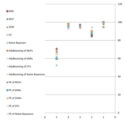
The detailed results of the proposed method
comparing with different classification algorithms are presented in Fig 3. To reach these results, 10
0 20 40 60 80 100 120
0 1
2 3
4 5
6 kNN
MLP SVM DT
Naïve Bayesian AdaBoosting of MLPs AdaBoosting of kNNs AdaBoosting of DTs
AdaBoosting of Naïve Bayesians PE of MLPs
PE of kNNs PE of SVMs PE of DTs
PE of Naïve Bayesians
independent runs of each algorithm are employed and their average accuracy is reported. In each run 66 random percent of dataset is considered as
train set and the rest 34% is considered as test set. The results still confirm that the proposed method is promising comparing with other classification algorithms including AdaBoosting. Fig 4 depicts a more detailed comparison between the proposed
method and Adaboosting method. It contains the result of Fig. 3 plus the confidence interval for
each method.
Fig. 5 compares the only AdaBoosting method with the proposed method. The results of the Fig 5 show that the proposed method can compete with AdaBoosting. The proposed method can
even outperform the AdaBoosting in some cases.
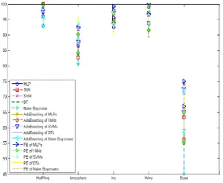
Fig. 4. Performance of different classification methods in terms of accuracy with the confidence interval.
V. CONCLUSION AND DISCUSSION Thanks to the good performance of the ensemble methods, they have been employed
in various applications. Generally in design of
combinational classifier systems, the more diverse the results of the classifiers, the more appropriate the final result. We propose a new method of creating an ensemble. It has been shown that the necessary diversity of an ensemble can be achieved by the proposed algorithm. The method was explained in detail above and the results
over some real data sets prove the correctness
of our claim. Although the ensemble created by proposed method may not always outperform all of the classifiers existing in ensemble, it always
possesses the diversity needed for creation of an
ensemble, and consequently it always outperforms the first or the simple classifier. We have also showed that time order of this mechanism is not
much more than simple methods. Indeed using
manipulation of data set features, we inject the necessary diversity in the ensemble; it means
this method is a type of generative methods that
manipulates data set in another way different with previous methods such as bagging and boosting.
REFERENCES
[1] L. Breiman,.: Bagging predictors. Machine Learning, 24(2): 123-140, 1996.
[2] E. Ghanbari, H. Beigy: Incremental RotBoost algorithm: An application for spam filtering. Intell. Data Anal. 19(2): 449-468, 2015.
[3] R.O Duda., P.E. Hart., and D.G. Stork.: Pattern Classification. 2nd ed. John Wiley & Sons, NY,.B. Smith, “An approach to graphs of linear forms (Unpublished work style),” unpublished. 2001.
[4] Q. Fu, S.X. Hu and S.Y. Zhao,.: A PSO-based approach for neural network ensemble. Journal of Zhejiang University (Engineering Science), 38(12): 1596-1600, 2004 (in Chinese).
[5] L. Breiman, Random forests, Mach. Learn. 45: 5–32, 2001.
[6] L. Breiman, Arcing classifiers, Annal. Stat. 26: 801–824, 1998.
[7] Y. Freund, and R.E. Schapire, “Experiments with a new boosting algorithm”, International Conference on Machine Learning, pp. 148–156, 1996.
[8] Y. Freund and R.E. Schapire ,”A
decision-theoretic generalization of on-line learning and
an application to boosting”, J. Comput. Sys. Sci. 55: 119–139, 1997.
[9] L.I. Kuncheva: Combining Pattern Classifiers, Methods and Algorithms, New York: Wiley, 2005.
[10] Lichman, M. (2013). UCI Machine Learning Repository [http://archive.ics.uci.edu/ ml]. Irvine, CA: University of California, School of Information and Computer Science.
[11] A. Lazarevic, and Z. Obradovic,: Effective pruning of neural network classifier ensembles. Proc. International Joint Conference on Neural Networks, 2: 796-801, 2001.
[12] Y. Liu, X.Yao: Evolutionary ensembles with negative correlation learning. IEEE Trans. Evolutionary Computation, 4(4): 380-387, 2000.
[13] P. Melville and R. Mooney: Constructing Diverse Classifier Ensembles Using Artificial
Training Examples. Proc. of the IJCAI-2003, p.505-510, 2003.
[14] B. Minaei-Bidgoli, G. Kortemeyer,
and W.F Punch.: Optimizing Classification Ensembles via a Genetic Algorithm for a Web-based Educational System. Lecture Notes in Computer Science 3138: 397-406, 2004.
[15] B. Minaei-Bidgoli, H. Parvin, H.
Alinejad-Rokny, H. Alizadeh, W.F Punch.: Effects of resampling method and adaptation on clustering ensemble efficacy. Artif. Intell. Rev. 41(1): 27-48 2014.
[16] H.D. Navone, P.F. Verdes, P.M. Granitto and H.A. Ceccatto: Selecting Diverse Members of Neural Network Ensembles. Proc. 16th Brazilian
Symposium on Neural Networks, p.255-260,
2000.
[17] D. Opitz, and J. Shavlik,: Actively searching for an effective neural network ensemble. Connection Science, 8(3-4): 337-353, 1996.
[18] H. Parvin, H. Helmi, B.
Minaei-Bidgoli, H. Alinejad-Rokny, and H. Shirgahi: Linkage Learning Based on Differences in Local Optimums of Building Blocks with One Optima. International Journal of the Physical Sciences 6(14): 3419–3425, 2011.
[19] H. Parvin, B. Minaei-Bidgoli, S. Ghatei, and H. Alinejad-Rokny,: An Innovative Combination of Particle Swarm Optimization, Learning Automaton and Great Deluge Algorithms for Dynamic Environments. International Journal of the Physical Sciences 6(22): 5121 – 5127, 2011.
[20] A. Krogh, and J. Vedelsdy,: Neural Network Ensembles Cross Validation, and Active Learning. Advances in Neural Information Processing Systems, 7: 231-238, 1995.
[21] H.R. Qodmanan, M. Nasiri, B.
Minaei-Bidgoli: Multi objective association rule mining with genetic algorithm without specifying minimum support and minimum confidence, Expert Systems with Applications, 38(1): 288-298, 2011.
[22] F. Roli and J. Kittler, Proc. of 2nd International Workshop on Multiple Classifier Systems, Vol. 2096 of Lecture Notes in Computer Science LNCS Springer- Verlag, Cambridge, UK, 2001.
[23] F. Roli and J. Kittler, Proc. of 3rd Int. Workshop on Multiple Classifier Systems, Vol. 2364 of Lecture Notes in Computer Science LNCS Springer Verlag, Cagliari, Italy, 2002.
[24] B.E. Rosen,: Ensemble learning using decorrelated neural network. Connection Science, 8(3-4): 373-384, 1996.
[25] R.E. Schapire,: The strength of weak learn ability. Machine Learning, 5(2):1971-227, 1990.
[26] Z.H. Zhou, J.X. Wu, Y. Jiang, and S.F. Chen: Genetic algorithm based selective neural network ensemble. Proc. 17th International Joint Conference on Artificial Intelligence, 2: 797-802,
2001.
[27] H. Parvin, B. Minaei-Bidgoli: A clustering ensemble framework based on selection of fuzzy weighted clusters in a locally adaptive clustering algorithm. Pattern Anal. Appl. 18(1): 87-112,
2015.
[28] M.H. Fouladgar, B. Minaei-Bidgoli, and H. Parvin: On Possibility of Conditional Invariant Detection. 6881(2): 214-224, 2011.
Alizadeh: Detection of Cancer Patients Using an Innovative Method for Learning at Imbalanced Datasets. LNCS 6954: 376-381, 2011.
[30] M. Daryabari, B. Minaei-Bidgoli, and H. Parvin: Localizing Program Logical Errors Using Extraction of Knowledge from Invariants. LNCS 6630: 124-135, 2011.
[31] H. Parvin, B. Minaei-Bidgoli and
S. Parvin: A Metric to Evaluate a Cluster by Eliminating Effect of Complement Cluster. LNCS 7006: 246-254, 2011.
[32] H. Parvin, B. Minaei-Bidgoli: Linkage Learning Based on Local Optima. LNCS 6922(1): 163-172, 2011.
[33] H. Parvin, B. Minaei-Bidgoli, and H.
Alizadeh and A. Beigi: A Novel Classifier Ensemble Method Based on Class Weightening in Huge Dataset. LNCS 6676 (2): 144-150, 2011.
[34] H. Parvin, B. Minaei-Bidgoli and H.
Ghaffarian: An Innovative Feature Selection Using Fuzzy Entropy. LNCS 6677 (3): 576-585,
2011.
[35] H. Parvin, B. Minaei, H. Karshenas, and