Divergence-free MHD Simulations with the HERACLES Code

(1)

DIVERGENCE-FREE MHD SIMULATIONS WITH THE HERACLES CODE

J. Vides

1

_{, E. Audit}

2

_{, H. Guillard}

3

_{et B. Nkonga}

4

Résumé. Au l des ans, la simulation numérique des équations de la magnétohydrodynamique (MHD) a joué un rôle important dans la recherche en physique des plasmas. La nécessité de trouver des solutions physiques et stables à ces équations a conduit à l'élaboration de plusieurs schémas numériques, tous devant satisfaire et préserver la contrainte de divergence nulle pour le champ magnétique numérique. Dans cet article, nous tenterons de montrer l'importance de maintenir cette contrainte numériquement. En particulier, nous étudions la technique de nettoyage hyperbolique de la divergence appliquée aux équations de la MHD idéale discrétisées sur une grille colocalisée et nous la comparons à la technique du transport constraint qui utilise une grille décalée pour maintenir cette propriété. Les méthodes sont implémentées dans le code HERACLES et des tests numériques sont présentés. Il est ainsi possible de comparer directement la robustesse et la précision des méthodes.

Abstract. Numerical simulations of the magnetohydrodynamics (MHD) equations have played a signicant role in plasma research over the years. The need of obtaining physical and stable solutions to these equations has led to the development of several schemes, all requiring to satisfy and preserve the divergence constraint of the magnetic eld numerically. In this paper, we aim to show the importance of maintaining this constraint numerically. We investigate in particular the hyperbolic divergence cleaning technique applied to the ideal MHD equations on a collocated grid and compare it to the constrained transport technique that uses a staggered grid to maintain the property. The methods are implemented in the software HERACLES and several numerical tests are presented, where the robustness and accuracy of the dierent schemes can be directly compared.

Introduction

The governing equations of magnetohydrodynamics (MHD) are used to model electrically conducting uid ows in the presence of magnetic elds. Given the ubiquity of these ows and the simplicity of the model, MHD has widespread application in both astrophysical and magnetically conned fusion plasmas. In the eld of plasma physics, the MHD model allows to treat plasma as a single conducting uid and describe dierent phenomena using macroscopic quantities and a corresponding system of conservation laws. Experimentally, these modeled phenomena are found to closely approximate aspects of real plasma behavior, such as MHD equilibria and stability, Alfvén waves, and eld line freezing, among others.

Therefore, it is not surprising that in the last few decades, the desire of performing highly ecient MHD simulations has become increasingly important. In order to have robust, accurate and stable solutions, it is necessary to satisfy the solenoidal property of the magnetic eld, which requires the magnetic eld to vanish 1 _{Inria, Maison de la Simulation, USR 3441, Gif-sur-Yvette, France. e-mail : [email protected]} 2 _{CEA, Maison de la Simulation, USR 3441, Gif-sur-Yvette, France.} _{e-mail : [email protected]}

3_{Université de Nice-Sophia Antipolis, UMR CNRS 7351 & Inria Sophia Antipolis, France. e-mail : [email protected]} 4_{Université de Nice-Sophia Antipolis, UMR CNRS 7351 & Inria Sophia Antipolis, France. e-mail : [email protected]}

c

EDP Sciences, SMAI 2013

(2)

everywhere at all times, while maintaining the conservation form of the fundamental physical laws. However, it is widely known that special care needs to be taken to satisfy and control this property on any numerical scheme, even if the magnetic eld is initially divergence-free. Failure to do so may result in nonlinear numerical instabilities and discretization errors increasing over time, manifesting themselves as discrepancies in the sim-ulations, e.g., incorrect jump conditions, wrong propagation speed of discontinuities, appearance of unphysical eects such as plasma transport orthogonal to the magnetic eld and negative pressures and/or densities.

The conservation law formulation of the MHD equations allows the use of Godunov-type schemes for their solution, and as a consequence, several strategies that aim to maintain the divergence-free property in mul-tidimensional Godunov-type codes have been developed over several years. In this paper, we focus on the divergence cleaning and constrained transport (CT) methods. The latter, originally introduced by Evans and Hawley [6], involves the use of a staggered magnetic eld, with its components dened at the cell interfaces. It is well known that this method provides a natural expression for the induction equation in conservative form. Hence, the combination of the CT framework with the Godunov one is an attractive solution, see [1,4,6,7], and this is the reason why it was the default and only technique used in the HERACLES code in order to perform MHD simulations. However, the staggered collocation of magnetic and electric eld variables, makes the use of this method in unstructured grids rather laborious and costly.

One of our future goals is to design a high order nite volume approximation for hyperbolic conservation laws in curvilinear unstructured grids. Given that HERACLES is currently a structured mesh code, we believe that other methods that do not involve a staggered grid will be simpler to extend to unstructured grids. Thus, we are motivated by the need to explore an alternative method and implement it in the HERACLES code. Among the dierent existing techniques, we choose to investigate the hyperbolic cleaning method introduced by Dedner et al. [5]. The main advantage of using this method is that it is easy to implement, since it is completely based on the cell-centered discretizations favored in Godunov schemes, and thus allows highly accurate solutions with reduced computational eort. We then compare both methods using several tests that aim to put in evidence their advantages and disadvantages.

This paper is organized as follows. In the next section, we review the governing equations for ideal MHD ows, which treat plasma as a perfectly conducting uid, and stress the importance of maintaining the divergence-free constraint at all times when performing numerical simulations. Some standard notation is introduced briey in Section 2. The details of the hyperbolic divergence cleaning method and the constrained transport methods are presented in Sections 3 and 4, respectively. Several numerical tests are presented and discussed in Section 5. Finally, concluding remarks are given in Section 6.

1. Governing equations and the divergence-free condition

The ideal MHD equations are a set of nonlinear hyperbolic equations in conservation form, given by

∂tρ+∇ ·(ρu) = 0, (1)

∂t(ρu) +∇ ·(ρu⊗u) +∇(p+1₂B·B)− ∇ ·(B⊗B) = 0, (2)

∂tε+∇ ·[(ε+p+1₂B·B)u−B(u·B)] = 0, (3)

∂tB+∇ ·(B⊗u−u⊗B) = 0, (4)

where ρ and u = (ux, uy, uz) are the uid density and velocity, respectively, and B = (Bx, By, Bz) is the

magnetic eld. Moreover, the magnetic eld satises the constraint

(3)

which will be discussed further below in Section 1.1. The total energy densityεand the thermal pressurepare

related through the ideal gas law

p= (γ₋1)

ε₋ρ

2u·u− 1 2B·B

,

which completes the set of equations. Unless stated otherwise, we will assume throughout the paper, that the specic heat capacity ratio γ is5/3. The evolution equation for the magnetic eld (4) is conveniently written in divergence form and it comes from Faraday's law:

∂tB+∇ ×E= 0, (6)

with the electric eld E given by the ideal Ohm's law

E=₋u_×B. (7)

1.1. Divergence constraint

The constraint ∇ ·B = 0 is not necessary in the time evolution in the sense that if the magnetic eld is assumed at the initial time step to be divergence-free, then an exact solution to the MHD equations will satisfy this condition for all timest >0. For smooth solutions, this is guaranteed by the evolution equation (4), since taking the divergence of the equivalent equation (6) and recalling that∇ ·(_{∇ × ·})_≡0, gives

∂t(∇ ·B) = 0.

As a result, from an analytical point of view, we sometimes nd in the literature that equation (5) is regarded as an involution rather than a constraint, as in [2,8]. Ideally, when performing numerical simulations, we would expect this particular equation to remain zero at all times. This is the case in one dimension, where the constraint becomes ∂xBx = 0 and the evolution equation for Bx in (4), decoupled from the other equations,

is reduced to ∂tBx = 0. Hence, an initial ∂xBx(·,0) = 0leads to∂xBx(·, t) = 0for all times t >0. However,

the matter is more complicated for multidimensional MHD ows. As detailed by the work of Brackbill and Barnes [3], numerical discretization errors have an impact on its time evolution in the following way:

∂t(∇ ·B) = 0 +O((∆x)m,(∆t)n),

where ∆xand ∆t are respectively the space and time discretization steps and m, n_≥1. In the same paper, Brackbill and Barnes show the importance of choosing an appropriate discretization of (5) in order to avoid the emergence of unwanted and unphysical eects in the MHD system. Basically, if∇ ·B₆= 0, the magnetic force

Fdened by

F=_{∇ ·}(B_⊗B)₋1

2∇(B·B), will not in general disappear in the direction of the magnetic eld, i.e.,

F_·B= (_{∇ ·}B)(B_·B)₆= 0.

(4)

2. General Notation

In this section, we introduce the notation as a standard for the numerical approximations of both the divergence cleaning and constrained transport techniques. We consider a uniform numerical grid in a three-dimensional domain with Cartesian coordinates (x, y, z). Henceforth, superscripts denote time levels and

sub-scripts refer to spatial location. The cell with center at (xi, yj, zk)is denoted by the integer subscripts (i, j, k)

and the centers of the cell's interfaces are denoted by half integers. We consider a system of conservation laws of the form

∂tU+∇ · F(U) = 0, (8)

with the uxF = (F,G,H). If we integrate this system in a grid cellxi−1/2≤x≤xi+1/2,yj−1/2≤y≤yj+1/2,

zk−1/2≤z≤zk+1/2 and over a time steptn ≤t≤tn+1, we obtain the following expression: Un+1

i,j,k=U n i,j,k−

∆t

∆x h

Fn

i+1/2,j,k−F n i−1/2,j,k

i

−_∆∆_yt hGn

i,j+1/2,k−G n i,j−1/2,k

i

−_∆∆_zthHn

i,j,k+1/2−H

n i,j,k−1/2

i

(9) where ∆x, ∆y and∆z are the mesh sizes in each direction and the time increment is given by ∆t, such that tn+1 = tn+ ∆t. In equation (9), both Uni,j,k and U

n+1

i,j,k are cell-averaged values of U at time t

n _and _tn+1_, respectively, and the uxes are obtained by a time-surface average. In a Godunov-type scheme, the uxes in equation (9) are evaluated by solving a one-dimensional Riemann problemRin the normal directionˆnat each

cell interface. Thus, in thex-direction, we have

Fn

i+1/2,j,k =F(R(0;Ui,j,k,Ui+1,j,k)) and Fin−1/2,j,k =F(R(0;Ui−1,j,k,Ui,j,k)), (10)

whereR(x/t;Ui,j,k,Ui+1,j,k)is the approximate solution of the Riemann problem atxi+1/2. Similar expressions can be found for the uxes in the remaining directions.

3. Hyperbolic divergence cleaning

When all variables dened in the hyperbolic system (1)-(4) are dened in the same position, a cleaning technique is needed to enforce the constraint ∇ ·B= 0. The hyperbolic divergence cleaning method suggested by Dedner et al. [5] is based on coupling the divergence constraint (5) to the evolution equation for the magnetic eld (4) by introducing a new scalar function or generalized Lagrangian multiplier (GLM)ψ. Then, both of the

mentioned equations, are replaced by

∂tB+∇ ·(B⊗u−u⊗B) +∇ψ = 0, (11)

D(ψ) +_{∇ ·}B = 0, (12)

withD(_·)being a linear dierential operator. Henceforth, the resulting system (1), (2), (3), (11), (12) is called the generalized Lagrange multiplier (GLM) formulation of the MHD equations, or simply, GLM-MHD. Dedner et al. analyzed dierent possibilities for Dand found that a satisfactory approximation to the original system

may be obtained by choosing a mixed hyperbolic/parabolic ansatz, which will be explained in detail in Section 3.1. Additionally, in order to obtain a good numerical approximation, it is necessary to choose adequate initial and boundary conditions for the unphysical variableψ(see Section 3.4). We keep the notation used by Dedner

et al. with few minor changes.

3.1. Linear dierential operator

D

Let us consider suciently smooth solutions. From equations (11) and (12), we can deduce that for any choice of D, the divergence of the magnetic eld and the scalar functionψ satisfy the same equation

∂tD(∇ ·B) −∆(∇ ·B) = 0, (13)

(5)

3.1.1. Parabolic correction

Dening the linear dierential operator as

D(ψ) = 1

c2

p

ψ, (15)

withcp∈(0,∞), and using it in (14) yields the heat equation∂tψ−c2p∆ψ= 0. Hence, this type of correction

allows for the perturbations in the magnetic eld to be dissipated and smoothed out, if appropriate boundary conditions are dened. However, the explicit approximation to the MHD equations using a parabolic correction presents certain diculties due to the restrictions imposed on the parametercp by stability conditions. Since

we are only interested in explicit schemes, we study more suitable operators. 3.1.2. Hyperbolic correction

We obtain a hyperbolic correction by choosing

D(ψ) = 1

c2

h

∂tψ, (16)

withch∈(0,∞). Substituting (16) into (14) gives the wave equation ∂tt2ψ−c

2

h∆ψ= 0. Thus, local divergence

errors are transported to the boundary with nite speedch. Now, if we express equation (12) in terms of the

hyperbolic correction, we obtain

∂tψ+c2h(∇ ·B) = 0, (17)

which is an attractive result since the resulting GLM-MHD system is purely hyperbolic. 3.1.3. Mixed correction

Formally, this approach is nothing but the combination of the parabolic and hyperbolic corrections, with the linear dierential operator dened by

D(ψ) = 1

c2

h

∂tψ+

1

c2

p

ψ, (18)

where cp and ch are the parabolic and hyperbolic constants previously dened. Direct substitution of this

correction into (14) leads to the telegraph equation ∂tt2ψ+c2h/c

2

p∂tψ =c2h∆ψ, which implies that the errors

associated to the divergence of the magnetic eld are both transported with speed ch and damped with time

and distance. Following the same approach used for the other corrections, from (14), we get

∂tψ+c2h(∇ ·B) =−

c2_h

c2

p

ψ, (19)

where it is evident that the damping comes now from a source term.

3.2. Eigensystem of the GLM-MHD equations

The complete GLM-MHD system with the mixed correction (18) can be written in the following form:

∂t

       

ρ

ρu

B

ε ψ

       

+_{∇ ·}

       

ρu

ρu_⊗u+ p+₂1B_·B_{I −}B_⊗B

B⊗u−u⊗B+ψ_I

(ε+p+1₂B_·B)u₋B(u_·B)

c2

hB

       

=

       

0 0

−c2h c2

pψ

       

(6)

where I is a 3_×3 identity matrix. This system, with a source term only in the equation for the unphysical variableψ, can be written in compact form as

∂tV+∇ · G(V) =S(V), (21)

with V = (ρ, ρu, B, ε, ψ)T and the ux function _G = (_Gx, Gy, Gz). Note that, in the limiting case where

cp → ∞, the mixed correction reduces to the hyperbolic one and S(V) = 0. Moreover, given the primitive

variables W= (ρ, ux, uy, uz, Bx, By, Bz, p, ψ)T, the homogeneous version of equation (21) may be rewritten in

the quasilinear form

∂tW+A(W)∂xW+B(W)∂yW+C(W)∂zW= 0, (22)

where, for example,

A(W) =

                  

ux ρ 0 0 0 0 0 0 0

0 ux 0 0 −B_ρx B_ρy B_ρz 1_ρ 0

0 0 ux 0 −

By

ρ −

Bx

ρ 0 0 0

0 0 0 ux −B_ρz 0 −B_ρx 0 0

0 0 0 0 0 0 0 0 1

0 By −Bx 0 −uy ux 0 0 0

0 Bz 0 −Bx −uz 0 ux 0 0

0 γp 0 0 (γ₋1)u_·B 0 0 ux (1−γ)Bx

0 0 0 0 c2_h 0 0 0 0

                  

. (23)

In the matrix Adened above, we see that it is possible to decouple the equations for Bx andψ from the

remaining system and solve them independently. Thus, for a one-dimensional problem, we obtain the following decoupled system of equations:

∂t

Bx

ψ !

+ 0 1

c2

h 0

!

∂x

Bx

ψ !

= 0

0

!

. (24)

Additionally, given W0 _{= (}_{ρ, u}

x, uy, uz, By, Bz, p)T, we dene the matrix A0(W0) by removing the fth and

ninth row and column fromA(W). ConsideringBxas a constant parameter, we get the quasilinear system

∂tW0+A0(W0)∂xW0= 0. (25)

It is well known that matrixA0_{is diagonalizable and has seven eigenvalues corresponding to one entropy wave} traveling with speed λ5=ux; two Alfvén waves traveling with speedλ3,7=u∓ca; and four magneto-acoustic

waves, two fast and two slow with speedsλ2,8=u∓cf andλ4,6=u∓cs, respectively, where

ca= |

Bx|

√_ρ, c2_f,s= 1 2



γp+B·B

ρ ±

s

γp+B_·B

ρ

2

−4γpB 2

x

ρ2



.

From the decoupled system, we obtain the eigenvalues λ1,9 =∓ch, which are distinct from the eigenvalues

ofA0 _{for a suciently large}_c

h. Therefore, the matrixAhas nine eigenvalues, such that

λ1≤λ2≤λ3≤λ4≤λ5≤λ6≤λ7≤λ8≤λ9.

(7)

3.3. Numerical approximation

In the previous section, we obtained the eigenvalues λ1,9 = ∓ch from the decoupled system, where the

constantchrepresents the propagation speed of local divergence errors. Thus,chis chosen to be the maximum

signal speed compatible with the time step ∆t, such that ch= max

i,j,k(|ux|+cf,x, |uy|+cf,y, |uz|+cf,z),

where cf,x, cf,y and cf,z are the fast magneto-acoustic speeds in the three directions. The time increment is

restricted by the Courant-Friedrichs-Levy (CFL) conditionccf l∈(0,1)in the following way:

∆t=ccf l

min(∆x,∆y,∆z)

ch

.

We attempt to solve equation (21), using the Godunov-type approach explained in Section 2. Hence, it is necessary to nd a numerical ux for the GLM-MHD system and we begin by deriving it for the hyperbolic GLM-MHD system, i.e., system (20) with no source terms. First, we notice that for arbitrary left and right states(Bx,L, ψL)and(Bx,R, ψR), the Godunov ux of system (24) can be computed exactly since

˜

Bx

˜

ψ !

= 1

2(Bx,L+Bx,R)− 1

2ch(ψR−ψL) 1

2(ψL+ψR)−

ch

2(Bx,R−Bx,L)

! .

Therefore we derive the numerical ux( ˜ψ, c2_hB˜x)T. For the remaining system, we use a seven-wave Riemann

solver Rfor the one-dimensional MHD equations with the normal component of the magnetic eld dened by ˜

Bx. Hence, the numerical uxG˜xhas the following form:

˜

Gx=Gx(R(0;VL,VR,B˜x),0) + (0,0,0,0,ψ,˜ 0,0,0, c2hB˜x)T, (26)

and, analogous expressions can be found for _G˜_y _and _G˜_z_{. Moreover, for the mixed GLM-MHD system, which} considers the source terms in the right-hand side of system (20), we use an operator-splitting approach. Thus, in the source step, we solve the initial value problem

∂tψ=−

c2

h

c2

p

ψ,

for which the initial conditionψ∗ is the output of the previous step. Integrating exactly for a time increment

∆t, yieldsψn+1₌_ψ∗_exp

−∆t c2

h/c

2

p

.Dedner et al. recommend xing the valuec2

p/ch= 0.18.

3.4. Boundary conditions

For the magnetohydrodynamic variables considered in system (1)-(4), the initial and boundary conditions are chosen according to the specic physical settings of the problem under consideration, but for the variableψ,

we are free to prescribe them. Given its nature, a good choice for the initial value of the unphysical variable is

ψ0_{= 0}_{. Regarding the particular choice of the boundary condition, Dedner et al. recommend assuming that the} behavior ofψandρis identical at the boundary, making the implementation quite simple and straightforward

on an existing code.

4. Constrained transport

(8)

the divergence-free property of the magnetic eld to machine round-o error precision. We use the notation introduced in Section 2. In order to avoid confusion, from now on, we denote the cell-centered magnetic eld by the usual capitalBand the staggered magnetic eld representation by a lowercaseb.

4.1. Staggered mesh discretization

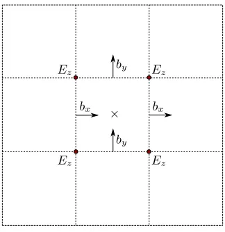
The staggered mesh formulation simply consists in dening the magnetic eld components at the cell inter-faces, the electric elds at the zone edges, and all the hydrodynamic variables at the centers. Figure 4.1 shows the collocation of the magnetic and electric eld in two dimensions, with the magnetic eld componentsbxand

bydened on the interface centers to which they are orthogonal. Thezcomponent of the electric eld is located

at the cell corners.

bx bx

by

×

Ez

Figure 4.1. Two-dimensional staggering in the constrained transport approach.

The main justication for using a staggered algorithm is that it allows to dene an inherently divergence-free method. Recalling Faraday's equation (6), it is clear that a discrete version of Stokes' theorem may be used to evolve in time a magnetic eld that has a staggered representation. Let us consider a cell (i, j) in two dimensions, with the staggered magnetic eld components dened by bx,i−1/2,j, bx,i+1/2,j, by,i,j−1/2 and

by,i,j+1/2. As mentioned above, the electric eld components are placed at cell corners . Hence, the induction equation is discretized along the cell edges as

bn_x,i+1₋₁_/₂_,j =bn_x,i₋₁_/₂_,j₋ ∆t

∆y

Ez,i−1/2,j+1/2−Ez,i−1/2,j−1/2

,

bn_x,i+1₊₁_/₂_,j =bn_x,i₊₁_/₂_,j₋ ∆t

∆y

Ez,i+1/2,j+1/2−Ez,i+1/2,j−1/2

,

bn_y,i,j+1₋₁_/₂=bn_y,i,j₋₁_/₂+ ∆t ∆x

Ez,i+1/2,j−1/2−Ez,i−1/2,j−1/2

,

bn_y,i,j+1₊₁_/₂=bn_y,i,j₊₁_/₂+ ∆t ∆x

Ez,i+1/2,j+1/2−Ez,i−1/2,j+1/2

.

(27)

If we dene the numerical divergence ∇ ·bfor cell (i, j)at timetn as

(_{∇ ·}b)n_i,j= b

n

x,i+1/2,j−b n x,i−1/2,j

∆x +

bn

y,i,j+1/2−b

n y,i,j−1/2

∆y , (28)

it is quite easy to show that an initial (_{∇ ·}b)n

i,j = 0 leads to (∇ ·b) n+1

i,j = 0, with machine round-o error

(9)

4.2. Numerical approximation

We briey describe a nite volume time-update strategy, with the purpose of showing the main steps needed to evolve the state variables over one time step. At the beginning of the time step, the hydrodynamic variables are dened at the center of the cells and the magnetic eldbat the corresponding interface centers. The initial

magnetic eld at the cell centerBi,j,kmay be approximately obtained in the following way:

Bx,i,j,kn =

bn

x,i−1/2,j,k+b n

x,i+1/2,j,k

2 , B

n y,i,j,k=

bn

y,i,j−1/2,k+b n

y,i,j+1/2,k

2 , B

n z,i,j,k =

bn

z,i,j,k−1/2+b

n

z,i,j,k+1/2

2 .

Let us denote the vector of centered variables by Un

i,j,k= (ρi,j,k, ρi,j,kui,j,k, εi,j,k,Bi,j,k)T.We then nd the

uxes at the faces by means of a seven-wave Riemann solver, as in (9), and make the update of the state vector Un

i,j,k using expression (10) in order to obtain U n+1

i,j,k. At this point, what remains is to update the magnetic

eld components at the faces. The main idea consists on constructing an approximation to the electric eld dened in (7) at the cell corners. This approximated electric eld is then used to update the face centered magnetic elds, by using a discrete version of Stokes' theorem, as shown in example (27).

A simple approach for the estimation of the electromotive force (EMF) at the cell edges is based on a simple spatial interpolation at time tn_{. In the following example, we approximate the EMF} _En

z,i−1/2,j−1/2 that is needed in (27). Thus,

E_z,in ₋₁_/₂_,j₋₁_/₂= ¯ux,i−1/2,j−1/2B¯y,i−1/2,j−1/2−u¯y,i−1/2,j−1/2B¯x,i−1/2,j−1/2, (29)

with

¯

ux,i−1/2,j−1/2=

un

x,i,j,k+u n

x,i−1,j,k+u n

x,i,j−1,k+u n

x,i−1,j−1,k

4 ,

¯

Bx,i−1/2,j−1/2=

Bn

x,i−1/2,j,k+B n

x,i−1/2,j−1,k

2 ,

¯

uy,i−1/2,j−1/2=

un

y,i,j,k+uny,i−1,j,k+uny,i,j−1,k+uny,i−1,j−1,k

4 ,

¯

By,i−1/2,j−1/2=

Bn

y,i,j−1/2,k+B n

y,i−1,j−1/2,k

2 .

It is important to mention that several and more complex methods have been proposed to update the magnetic elds at the interface centers. We refer the reader to [1,6,7,9,14].

5. Numerical results

The numerical implementation of both methods presented in this paper has been done in the HERACLES code for astrophysical uid ows. By having a common computational framework, we can fairly compare the accuracy and robustness of the hyperbolic divergence cleaning and constrained transport techniques. Thus, in this section, we present a series of selected test problems. We note that the divergence of the magnetic eldB

for cell (i, j, k)at timetn is computed as

(_{∇ ·}B)ni,j,k=

Bn

x,i+1,j,k−B n x,i−1,j,k

2∆x +

Bn

y,i,j+1,k−B n y,i,j−1,k

2∆y +

Bn

z,i,j,k+1−B

n z,i,j,k−1

2∆z . (30)

For second order approximations, we extend the hyperbolic cleaning scheme by using the MUSCL-Hancock Method (MHM), see [13]. In the case of the constrained transport, the MUSCL-Hancock approach detailed in [7] is employed. As for the choice of slope limiters, we use the MinMod limiter since it is known to ensure the positivity of the solution in multiple space dimensions.

5.1. Advection in

B

x

(10)

In the contour plots shown in Figure 5.1, we can perceive that during the time evolution, the initial peak in

Bxdecreases in height for both the hyperbolic and mixed cleaning, but is well advected with the ow velocity

nonetheless. The mixed GLM solutions do not show the complex wave interactions seen in the hyperbolic case, because of the additional damping. Additionally, this problem also allows to nd the optimal value for the ratio

c2

p/ch= 0.18(see Figure 5.2).

Advection inBx

Computational domain: [−0.5,1.5]×[−0.5,1.5]; Periodic boundaries

ρ ux uy uz Bx By Bz p

1.0 1.0 1.0 0.0 r(x2+y2)/√4π 0.0 1/√4π 6.0

r(s) =

(

4096s4₋₁₂₈_s2_{+ 1} _if_s_∈_[0_,₀_._125]_,

0 otherwise.

Table 1. Initial data for the peak inBxproblem described in [5].

0.0 0.5 1.0 x 0.0

0.5 1.0

y

−0.0908

−0.0442 0.0024 0.0490 0.0957 0.1423 0.1889 0.2355 0.2821 Bxcomponent of the magnetic fieldatt= 0.25003s

0.0 0.5 1.0 x 0.0

0.5 1.0

y

(a) t= 0.25

0.0 0.5 1.0 x 0.0

0.5 1.0

y

−0.0908

0.0 0.5 1.0 x 0.0

0.5 1.0

y

(b)t= 0.50

0.0 0.5 1.0 x 0.0

0.5 1.0

y

−0.0908

0.0 0.5 1.0 x 0.0

0.5 1.0

y

(c)t= 0.75

0.0 0.5 1.0 x 0.0

0.5 1.0

y

−0.0908

0.0 0.5 1.0 x 0.0

0.5 1.0

y

(d)t= 1.0

Figure 5.1. Isolines ofBx obtained with the HLLD scheme. The computations are performed with

256×256points for hyperbolic and mixed GLM approaches (from top to bottom).

0.10 0.15 0.20 0.25 0.30 0.35 0.40 0.45 0.50 cr

0.010 0.015 0.020 0.025 0.030 0.035 0.040

Time average of the total divergence

(a)64×64points

0.10 0.15 0.20 0.25 0.30 0.35 0.40 0.45 0.50 cr

0.010 0.015 0.020 0.025 0.030 0.035 0.040

(b)128×128points

0.10 0.15 0.20 0.25 0.30 0.35 0.40 0.45 0.50 cr

0.010 0.015 0.020 0.025 0.030 0.035 0.040

(c)256×256points

Figure 5.2. Time averages of the total divergence obtained with the HLLD scheme for problem 5.1

(11)

5.2. Orszag-Tang

The Orszag-Tang vortex is a standard and well-known 2D test for MHD codes. It describes a periodic uid conguration with initial conditions that lead to a system of supersonic MHD turbulence (see Table 5.2). Thus, this problem allows to test the dierent methods' ability to handle such turbulence and MHD shocks.

Orszag-Tang

Computational domain:[0,1]×[0,1]; Periodic boundaries

γ2 ₋_sin(2_πy₎ _sin(2_πx₎ ₀_.₀ ₋_sin(2_πy₎ _sin(4_πx₎ ₀_.₀ _γ

Table 2. Initial data for the Orszag-Tang vortex described in [10].

Density distributions at times t = 0.5 and t = 1.0 are shown in Figure 5.3, where we can visualize the formation of small scale vortices and turbulence. The good agreement between our results and the ones obtained in previous investigations, such as in [4,7, 10,11,14], is satisfactory.

0.2 0.4 0.6 0.8 x 0.2

0.4 0.6 0.8

y

1.5 2.0 2.5 3.0 3.5 4.0 4.5 5.0 5.5

Densityρatt= 0.50002s

0.2 0.4 0.6 0.8 x 0.2

0.4 0.6 0.8

y

0.8 1.2 1.6 2.0 2.4 2.8 3.2 3.6 4.0

(a) No correction

0.2 0.4 0.6 0.8 x 0.2

0.4 0.6 0.8

y

1.5 2.0 2.5 3.0 3.5 4.0 4.5 5.0 5.5

0.2 0.4 0.6 0.8 x 0.2

0.4 0.6 0.8

y

0.8 1.2 1.6 2.0 2.4 2.8 3.2 3.6 4.0

(b) Hyperbolic GLM

0.2 0.4 0.6 0.8 x 0.2

0.4 0.6 0.8

y

1.5 2.0 2.5 3.0 3.5 4.0 4.5 5.0 5.5

0.2 0.4 0.6 0.8 x 0.2

0.4 0.6 0.8

y

0.8 1.2 1.6 2.0 2.4 2.8 3.2 3.6 4.0

(c) Mixed GLM

0.2 0.4 0.6 0.8 x 0.2

0.4 0.6 0.8

y

1.5 2.0 2.5 3.0 3.5 4.0 4.5 5.0 5.5

0.2 0.4 0.6 0.8 x 0.2

0.4 0.6 0.8

y

0.8 1.2 1.6 2.0 2.4 2.8 3.2 3.6 4.0

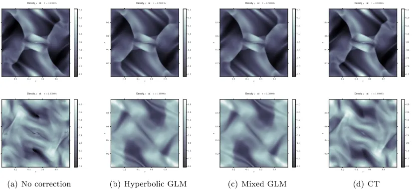
(d) CT Figure 5.3. 2D density plots, rst order in both space and time, for the Orszag-Tang system using

256×256points at timest= 0.5(top) andt= 1.0(bottom).

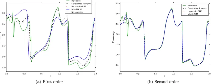
In Figure 5.4, the evolution of the L1 _{norm and maximum value of the divergence is plotted for dierent} cell-centered techniques. It is evident that the measuredL1_{errors for the hyperbolic and mixed approaches seem} to converge to zero as time increases, while those obtained without correction tend to increase with time. We note that a second order simulation with no correction is not possible to obtain since the blow-up of divergence errors causes the crash of the simulation. In Figure 5.5, we show horizontal cuts aty = 0.3125of the pressure distribution, and nd no perceivable dierence between the hyperbolic and mixed GLM techniques. Moreover, the same gure allows to conclude that the constrained transport method solves this problem more accurately than the divergence cleaning techniques presented in this paper.

5.3. Kelvin-Helmholtz Instability

(12)

0.0 0.2 0.4 0.6 0.8 1.0

t

0.0 0.5 1.0 1.5 2.0 2.5

L

1(∇

·

B

)

Hyperbolic GLM Mixed GLM No correction

0.0 0.2 0.4 0.6 0.8 1.0

t

0 50 100 150 200 250

m

ax

(

∇

·

B

)

Figure 5.4. L1(∇ ·B)(left) andmax(∇ ·B)(right) obtained with the HLLD scheme for the

Orszag-Tang vortex. The computations are performed using a cell-centered approach on256×256points.

0.0 0.2 0.4 0.6 0.8 1.0

x

0.5

1.0

1.5

2.0

2.5

3.0

P

re

s

u

re

p

Reference Constrained Transport Hyperbolic GLM Mixed GLM No correction

(a) First order

0.0 0.2 0.4 0.6 0.8 1.0

x

0.5

1.0

1.5

2.0

2.5

3.0

3.5

P

re

s

u

re

p

Reference Constrained Transport Hyperbolic GLM Mixed GLM

(b) Second order

Figure 5.5. Horizontal cut aty= 0.3125showing the gas pressurepin the Orszag-Tang system at

t= 0.5using the HLLD scheme and256×256points. The solid green line gives a reference solution

obtained with a second-order constrained transport algorithm on a ner grid of1024×1024points.

Kelvin-Helmholtz Instability

Computational domain: [0,1]×[−1,1]

Boundaries: reexive on top and bottom, periodic on left and right

1.0 M/2(tanh(20y)) 0.0 0.0 ca

√

ρcos(θ) 0.0 ca

√

ρsin(θ) 1/γ

θ=π/3, M = 1, ca= 0.1, σ= 0.1

Single mode perturbation: uy(x, y) = 0.1 sin(2πx)(e−y

2_/σ2

)

(13)

Figure 5.6. Initial single mode perturbationuy(x, y)for the Kelvin-Helmholtz instability.

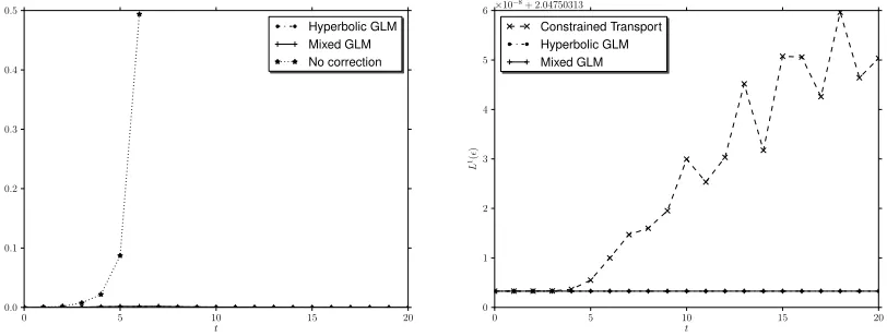
The left plot in Figure 5.7 shows the L1 _{norm of the divergence}

∇ ·B at dierent times for the methods

that use a cell-centered collocation. For the case without correction, a blow-up of divergence errors occurs, causing the simulation to crash. This problem is then addressed by adding a divergence cleaning technique. Additionally, on the right plot, we present the time evolution of the L1 _{norm of the total energy density} _ε_{, a} conserved quantity in the MHD equations. However, for the constrained transport method, there is a slight loss of the conservation at the level of discretization error.

0 5 10 15 20

t

0.0

0.1

0.2

0.3

0.4

0.5

L

1(∇

·

B

)

0 5 10 15 20

t 0

1 2 3 4 5 6

L

1(ǫ

)

×10−8_{+ 2}_._04750313

Constrained Transport Hyperbolic GLM Mixed GLM

Figure 5.7. L1₍_{∇ ·}_B₎ _{(left) and} _L1₍_ε₎ _{(right) obtained with the HLLD scheme for the}

Kelvin-Helmholtz instability. The computations are performed using256×256points.

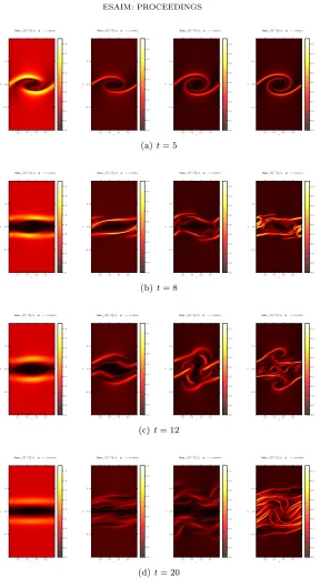
Evolution plots are shown in Figure 5.8 for the ratio of the poloidal eld strength and the toroidal component

q

B2

x+B2y/Bz. For all the methods analyzed, in the rst ve seconds we perceive the formation of the typical

(14)

0.2 0.4 0.6 0.8 x

−0.5 0.0 0.5

y

0.0 0.2 0.4 0.6 0.8 1.0 1.2 1.4 1.6 1.8 RatiopB2x+B2y/Bzatt= 5.00024s

0.2 0.4 0.6 0.8 x

−0.5 0.0 0.5

y

0.2 0.4 0.6 0.8 x

−0.5 0.0 0.5

y

0.2 0.4 0.6 0.8 x

−0.5 0.0 0.5

y

(a)t= 5

0.2 0.4 0.6 0.8 x

−0.5 0.0 0.5

y

0.0 0.2 0.4 0.6 0.8 1.0 1.2 1.4 1.6 1.8 RatiopB2

x+B2 y/Bzatt= 8.00036s

0.2 0.4 0.6 0.8 x

−0.5 0.0 0.5

y

0.0 0.6 1.2 1.8 2.4 3.0 3.6 4.2 4.8 5.4 RatiopB2

0.2 0.4 0.6 0.8 x

−0.5 0.0 0.5

y

0.0 0.8 1.6 2.4 3.2 4.0 4.8 5.6 6.4 7.2 RatiopB2

0.2 0.4 0.6 0.8 x

−0.5 0.0 0.5

y

0.0 0.8 1.6 2.4 3.2 4.0 4.8 5.6 6.4 7.2 RatiopB2

(b)t= 8

0.2 0.4x0.6 0.8

−0.5 0.0 0.5

y

0.2 0.4x0.6 0.8

−0.5 0.0 0.5

y

0.2 0.4x0.6 0.8

−0.5 0.0 0.5

y

0.2 0.4x0.6 0.8

−0.5 0.0 0.5

y

(c)t= 12

0.2 0.4 0.6 0.8 x

−0.5 0.0 0.5

y

0.0 0.2 0.4 0.6 0.8 1.0 1.2 1.4 1.6 1.8 RatiopB2

x+B2 y/Bzatt= 20.00000s

0.2 0.4 0.6 0.8 x

−0.5 0.0 0.5

y

0.0 0.6 1.2 1.8 2.4 3.0 3.6 4.2 4.8 5.4 RatiopB2

x+B2 y/Bzatt= 20.00000s

0.2 0.4 0.6 0.8 x

−0.5 0.0 0.5

y

0.0 0.8 1.6 2.4 3.2 4.0 4.8 5.6 6.4 7.2 RatiopB2

x+B2 y/Bzatt= 20.00000s

0.2 0.4 0.6 0.8 x

−0.5 0.0 0.5

y

0.0 0.8 1.6 2.4 3.2 4.0 4.8 5.6 6.4 7.2 RatiopB2

x+B2 y/Bzatt= 20.00000s

(d)t= 20

Figure 5.8. Evolution of the Kelvin-Helmholtz instability obtained with the HLLD scheme for the mixed GLM, constrained-transport, second order mixed GLM, and second order constrained-transport (from left to right). The results for the hyperbolic GLM (not shown) are almost identical to those obtained with the mixed GLM technique. The plots show the ratio of the poloidal eld strength and

the toroidal component, i.e.,p

B2

(15)

6. Conclusions

In this paper, we have investigated and compared two dierent methods that aim to maintain the divergence-free property of the magnetic eld, a constraint that cannot be ignored without having consequences.

The method proposed by Dedner et al. [5] prescribes a hyperbolic equation that allows for the divergence errors to be propagated to the boundary of the domain. The same authors recommend using a small variation of this approach, the mixed GLM ansatz, which oers both propagation and damping of the errors. The advantage of the divergence cleaning technique is that it is easy to implement as it is based on the cell-centered formulation favored in the Godunov approach. However, one disadvantage is that it depends on tunable parameters.

On the other hand, the constrained transport (CT) approach, originally introduced by Evans and Hawley [6], relies on a staggered formulation of the magnetic and electric elds. One clear advantage of this method is its inherently divergence-free magnetic eld. Moreover, it does not have tunable parameters, as in the hyperbolic divergence cleaning technique. However, this method is harder to implement and it sometimes presents loss of the conservation of the total energy density.

Through the dierent numerical test cases, we have shown that the implementation of the hyperbolic diver-gence cleaning approach in the HERACLES code was successful. This has allowed us to compare both methods and comment on the advantages and disadvantages that they possess. We were able to reproduce quantitatively results obtained by several authors and found that both methods are robust and ecient. Although we nd that the hyperbolic divergence cleaning generates more diusive results than the constrained transport method, the simplicity of the method makes it an attractive technique for our future work in the design of a high order nite volume approximation for hyperbolic conservation laws in curvilinear unstructured grids.

References

[1] D. S. Balsara and D. S. Spicer. A staggered mesh algorithm using high order Godunov uxes to ensure solenoidal magnetic elds in magnetohydrodynamic simulations. Journal of Computational Physics, 149(2):270292, 1999.

[2] T. Barth. On the role of involutions in the discontinuous Galerkin discretization of Maxwell and magnetohydrodynamic systems. In Compatible Spatial Discretizations, volume 142 of The IMA Volumes in Mathematics and its Applications, pages 6988. Springer New York, 2006.

[3] J. U. Brackbill and D. C. Barnes. The eect of nonzero∇·Bon the numerical solution of the magnetohydrodynamic equations.

Journal of Computational Physics, 35(3):426430, 1980.

[4] W. Dai and P. R. Woodward. On the divergence-free condition and conservation laws in numerical simulations for supersonic magnetohydrodynamical ows. The Astrophysical Journal, 494(1):317, 1998.

[5] A. Dedner, F. Kemm, D. Kröner, C.-D. Munz, T. Schnitzer, and M. Wesenberg. Hyperbolic divergence cleaning for the MHD equations. Journal of Computational Physics, 175(2):645673, 2002.

[6] C. R. Evans and J. F. Hawley. Simulation of magnetohydrodynamic ows: a constrained transport method. Astrophysical Journal, Part 1, 332:659677, September 1988.

[7] S. Fromang, P. Hennebelle, and R. Teyssier. A high order Godunov scheme with constrained transport and adaptive mesh renement for astrophysical MHD. A&A, 457:371384, 2006.

[8] C. Helzel, J. A. Rossmanith, and B. Taetz. An unstaggered constrained transport method for the 3D ideal magnetohydrody-namic equations. Journal of Computational Physics, 230(10):38033829, 2011.

[9] P. Londrillo and L. Del Zanna. High-order upwind schemes for multidimensional magnetohydrodynamics. The Astrophysical Journal, 530(1):508, 2000.

[10] A. Mignone, P. Tzeferacos, and G. Bodo. High-order conservative nite dierence GLMMHD schemes for cell-centered MHD. Journal of Computational Physics, 229(17):58965920, 2010.

[11] T. Miyoshi and K. Kusano. A multi-state HLL approximate Riemann solver for ideal magnetohydrodynamics. Journal of Computational Physics, 208(1):315344, 2005.

[12] K. G. Powell. An approximate Riemann solver for magnetohydrodynamics (that works in more than one dimension). Technical Report 94-24, ICASE, Langley, VA, 1994.

[13] E. F. Toro. Riemann Solvers and Numerical Methods for Fluid Dynamics: A Practical Introduction. Springer, 2009. [14] G. Tóth. The ∇ ·B = 0 constraint in shock-capturing magnetohydrodynamics codes. Journal of Computational Physics,

161(2):605652, 2000.