I S A V
Journal of Theoretical and Applied
Vibration and Acoustics
journal homepage: http://tava.isav.ir
Adhesive joint modeling using compatible element formulation
Mohammad Hossein Malakooti
a,
Hamid Ahmadian
a,
Hassan Jalali
b*a
School of Mechanical Engineering, Iran University of Science and Technology, Tehran, Iran b
Department of Mechanical Engineering, Arak University of Technology, Arak, Iran
A R T I C L E I N F O A B S T R A C T
Article history:
Received 7 November 2015
Received in revised form 29 February 2016
Accepted 24 June 2016
Available online 10 August 2016
The use of structural adhesives in automotive structures has been increased recently for their role in noise, vibration and harshness (NVH). Therefore, the dynamic behavior of structures containing bonded joints has become an area with numerous investigations over the past decades. Development of accurate formulations capable of representing adhesively bonded joint dynamics is a step forward in constructing the numerical models for one of the most useful kinds of joints in industry. Analysis of the adhesive layer between the two parts requires special assumptions which leads to using nonlinear and three dimensional models. Obtaining shape functions for an adhesive element by using finite element (F.E.) theory is a complicated and difficult task to do. The complexity is increased when it is assumed that the adhesive element is compatible with the plate element. In this paper, a new finite element formulation is developed for the adhesive layer which does not rely on shape functions and is compatible with the plate element. The accuracy of the proposed element is evaluated by using numerical and experimental results.
©2016 Iranian Society of Acoustics and Vibration, All rights reserved. Keywords:
Finite element method
Adhesively bonded joints Natural frequencies
1. Introduction
The use of adhesive bonding as chemical welding has many advantages such as easy and flexible fabrication, good sealing, lightness, heat and sound isolation and also corrosion resistance. Additionally, the side effects on materials such as the thermal effects in welding or creating holes in the structure for bolted or riveted joints, are not present in adhesive bonding. These capabilities increase the desire for using the adhesive bonding as an excellent option for design and maintenance purposes. There are many important issues to consider as the designer or technical user of adhesive bonding: strength, durability and deformation of the adhesive as well
* Corresponding Author.
E-mail address: [email protected] (H. Jalali)
134 as their dynamic responses. Hence, a reliable and economic model is needed to express the realistic behavior of adhesive joints physically.
There are two general approaches for theoretical analysis of adhesively bonded joints: closed-form and numerical analyses. The expenses of experimental tests on structures encourages engineers to develop closed-form or numerical expressions of the problem. Valuable studies have been performed on closed-form solutions from 1960 to 1990 by setting differential equations and applying the boundary conditions in formulations. A comparative literature review on analytical models for adhesive joints was performed by Lucas da Silva et al. [1]. The review shows that almost all analytical models for adhesively bonded lap joints are two-dimensional. In a companion paper, they compared the analytical models with experimental results [2]. The closed-form solutions are able to give the stress and displacements in some points of the adhesive bonding but are limited to simple geometries. Numerical methods, as a general tool for analysis, are used to solve the differential equations approximately with an acceptable accuracy. The finite element method is used as the most applicable and powerful method among other numerical methods due to its many benefits.
Dynamic analysis of structures containing adhesive joints has been investigated by many researchers in the literature through finite element modelling. For the case of modeling the adhesive layer using the finite element method, there are two general approaches. The first approach consists of using one layer of solid elements per composite ply linked together with the interface elements [3] . The second approach considers adopting one multi-layered shell element through the laminate thickness [4]. Kaya et al. [5] studied the effects of different dynamic characteristics in the adhesively bonded joints subjected to dynamic forces by using 3D F.E.A. They used the eight node brick elements and modelled the joint as a thin plate clamped from the left side. Then, the in-plane vibration analysis is constructed and the natural frequencies and mode shapes are measured.
He [6] used the finite element method and investigated the free torsional vibration characteristics of adhesively bonded single-lap joints. In this work, 20-node quadratic brick solid elements are used for modelling the adhesive joint and the results of the F.E. model are validated by experimental modal analysis. He concluded that the adhesive properties have a great influence on the torsional natural frequency and mode shapes of the structure.
Nobari and Jahani [7], Jahani and Nobari [8] and Naraghi and Nobari [9] employed the finite element method for identification of different dynamic characteristics of adhesive joints. They have used measured modal properties in the identification process.
135 As discussed above, adherents and adhesive are usually modelled in bounded structures by using solid elements. This type of modeling is not computationally efficient especially when adhesive joint is used between two plate substructures. In these circumstances, the plate substructures can be efficiently modeled by plate elements. Therefore a suitable element which is compatible with the plate element should be used to model the adhesive. The aim of this paper is to propose a new approach for finite element formulation of adhesive joint being compatible with the plate element.
The paper is arranged as follows: section 2 describes the challenging problem of modeling an adhesive layer. Finite element formulation for a new adhesive element is introduced in section 3. In section 4, numerical and experimental case studies are given to show the accuracy of the proposed model. Finally, conclusions are drawn and references are outlined.
2. Problem statement and solution method
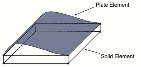
The aim of this paper is to obtain a proper finite element representation for the adhesive layer between two sheets which are modeled by plate elements as adherents. The common element usually used to consider the adhesive layer in finite element models is the solid element. Two problems arise when modeling the adhesive and the adherents by the combination of solid and plate elements. Firstly, the plate element has two rotational and one translational degree of freedom per node while the solid element has three translational degrees of freedom per node. Assembling these two elements, i.e. the plate and solid elements, gets complicated at their interface and leads to a gap along the elements’ edges as is shown in Fig. 1. This gap is due to the inconsistency between the displacement fields of these two elements.
Fig. 1. The gap between the solid element (as adhesive) and plate the element (as adherent)
Secondly, when solid elements are used for modelling the adhesive layer, experimental and finite element results are seldom found matching in all modes. This is especially true for torsional modes. The main advantages of modelling the adhesive layers for composite structures in torsion or bending by compatible elements are reducing the number of elements and thus the cost of calculations and increasing the accuracy of the results in torsional modes.
136 of the adhesive layer are not fully known, the approaches used in the finite element method are inapplicable to constructing a finite element formulation for the adhesive joint.
One approach for modeling the adhesive layer is to use the solid element having rotational degrees of freedom. To have a solid element with rotational degrees of freedom, the rotation defined by Allman can be used [13, 14]. The nodal rotation used in Allman’s interpolation is not in conformity with the continuum-defined rotation. Also, some zero energy modes are observed when this definition is used for rotation of corner nodes. In fact, when all the nodal rotations about any particular axis assume the same value, strain-free modes appear which are interpreted as the equal-rotation modes [15]. These drawbacks make this element inappropriate for modeling the adhesive layer. The shape functions and the stiffness matrix formulation for the solid element with Allman defined rotation degrees of freedom can be found in several studies [15-18].
In following section, a new formulation for finite element modelling of adhesive joints is proposed. For this end, the displacement field of the adhesive layer element is considered as a combination of the displacement fields of the upper and lower plate elements.
3. Joint element formulation
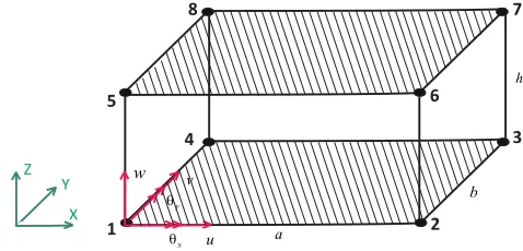
As stated in the previous section, the new joint element should be compatible with the plate elements in its upper and lower surfaces. Therefore, corresponding with the plate element, the rotational degrees of freedom are needed at each node. Since brick elements are usually used in modeling the adhesive in bounded structures, we consider that the joint element as an 8-noded/5-DOFs brick element as is shown in Fig. 2. The nodal 8-noded/5-DOFs vector is considered as
T y x w v
u, , , , ]
[ . One advantage of considering such a nodal DOFs vector is that the element is compatible with the plate elements in its lower and upper surfaces. In the following, the proper displacement field is developed for this joint element by using the shape functions of the upper and lower plate elements.
Fig. 2. the brick element (abh) with rotational degrees of freedom
The joint element shown in Fig. 2 is considered to be composed of two plate elements. The lower plate element consisting of nodes 1, 2, 3 and 4 is located at z0 and its displacement field is
( , )
( , ), ( , ), ( , )
TL L L L
Y x y u x y v x y w x y
. The upper plate element composed of nodes
5, 6, 7 and 8 is located at z h and its displacement field is
T U
U U
U x y u x y v x y w x y Y ( , )} [ ( , ), ( , ), ( , )]
{ . ui, vi and wi with iL U, may be expressed as,
1 5
8 7
3
2 6 4
X Y
Z w
x q
y
q
a
b h
137 4 4 3 3 2 2 1
1( , ) ( , ) ( , ) ( , )
) ,
(x y N x y u N x y u N x y u N x y u
uL (1)
4 4 3 3 2 2 1
1( , ) ( , ) ( , ) ( , )
) ,
(x y N x y v N x y v N x y v N x y v
vL (2)
4 1 3 1 3 23 ( , ) ( , ) ( , ) )
( ) , ( j yj j xj j j j
L x y N x y w N x y N x y
w (3)
The same relations can be developed for uU, vU and wU. In Eqs. (1-3) Ni(x,y), i1,2,...,4 and
12 ,..., 2 , 1 ), ,
(x y i
Ni are the shape functions corresponding to in-plane and lateral deformations
of a plate element which are given in the Appendix [19].
In this paper we consider the displacement field of the joint element as a combination of the displacement fields of the lower and the upper plate elements as:
)} , ( ){ ( )} , ( ){ ( )} , , (
{Y x y z f z YL x y g z YU x y (4)
where T
z y x w z y x v z y x u z y x
Y( , , )} [ ( , , ), ( , , ), ( , , )]
{ . f(z) and g(z) are governed by the
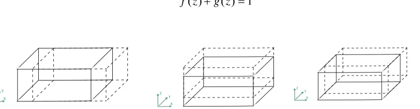
element properties and specially its rigid body modes. The joint element has six rigid body modes: three translational and three rotational. Three translational rigid body modes of the joint element are presented in Fig. 3. The translational rigid body modes can be expressed mathematically as, { ( , )} { ( , )} )} , , (
{Y x y z YL x y YU x y (5)
By substituting Eq. (5) into Eq. (1), the first constraint on functions f(z) and g(z) is obtained
as,
1 ) ( )
(z g z
f (6)
Fig. 3. Translational rigid body modes of the joint element
138
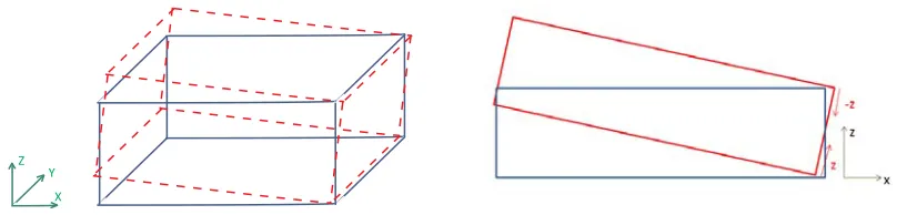
Fig. 4. Two different views of a rotational rigid body mode
The second constraint on functions f(z) and g(z) is obtained in the following by using the
rotational rigid body mode about y axis. Rotation about the y axis results in displacement along the x direction, i.e. u(x,y,z) for the joint element. Since the positive local z axis of the lower
plate element and the negative local z axis of the upper plate element contribute in constructing
the displacement along x direction, by using Fig. (4), u(x,y,z) can be expressed as, )
, ( ) ( ) , ( ) ( ) , ,
(x y z f z x y g z x y
u yL yU (7)
where yL(x,y)yU(x,y) is the rotation about y axis. On the other hand, a strain free- or
rigid body- mode is obtained when,
) , ( ) / 1 ( ) , ( / ) , ,
(x y z z h x y z h x y
u yL yU (8)
Eqs. (7) and (8) are identical which result in the second constraint on functions f(z) and g(z)
as,
1 / 2 ) ( )
(z g z z h
f (9)
Solving Eqs. (2) and (9) simultaneously yields to the proper f(z) and g(z) functions.
Therefore, the unique combination of the lower and upper plate elements’ displacement fields as the displacement field of the joint element is obtained as,
)} , ( ){ / ( )} , ( ){ / 1 ( )} , , (
{Y x y z z h YL x y z h YU x y (10)
The displacement field presented in Eq. (10) can be used to construct the finite element formulation of the joint element [19]. The stress-strain relation of the joint element is
}
]{
[
}
{
D
and the joint stiffness matrix is obtained by using Eq. (11),
V
T
J B D B dV K ] [ ] [ ][ ]
[
(11)
where [D] and [B] are respectively the constitutive and strain-displacement matrices. In the following section, the numerical simulation and experimental validation of the proposed adhesive joint element are presented.
139
4. Numerical simulation and experimental validation
The proposed model in the previous section is used in construction of F.E. models of two structures: adhesive layer as a connection of a plate to foundation and an adhesively bonded joint of two plates. The capability of the proposed model in representing the dynamic properties of these structures is investigated in the remaining of this section.
4.1. Numerical simulation: Panel bonded to the foundation
The structure considered in this section is a rectangular steel plate with dimensions of a=30 cm
and b=20 cm. A layer of adhesive is used to clamp the plate to its underlying surface as shown in
Fig. 5. The thickness of the plate is 1 mm and the thickness of the adhesive layer is t 2m m
along all sides.
Fig. 5. Panel bonded to the foundation using adhesive
First, a finite element model of this structure was constructed in MSC.NASTAN® employing QUAD4 elements for modelling the plate and HEX8 elements for modeling the adhesive layer. HEX8 is an 8-noded/3DOFs solid element. 400 solid elements were used in the MSC.NASTAN® finite element model to represent the adhesive layer. The material properties used in F.E. modelling for steel plate and adhesive joint are tabulated in table 1. The adhesive was considered Sikaflex 252 which will be later used in experimental case study.
Table 1. Adhesive and steel plate material properties
Young Modulus (GPa) Poisons’ Ratio Density (Kg/m3)
Steel plate 210 0.3 7800
Adhesive 3 0.34 1140
The optimum number of elements was used for modelling the steel plate such that increasing the element numbers did not change the natural frequencies. The first three natural frequencies of this structure are presented in Table 2.
140
Table 2. First three natural frequencies in (Hz) obtained from different F.E. adhesive modelling approaches
1st mode 2nd mode 3rd mode
MSC.NASTRAN model 552.62 720.84 1023.16
Solid element with Allman rotation 562.00 742.00 1011.00
Proposed joint model 560.00 727.00 1034.00
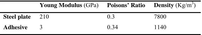
The capability of the solid element with Allman rotational degrees of freedom and the proposed joint model in this paper in representing the dynamics of the above structure was investigated next. For this purpose, a finite element model with fewer elements for modelling the adhesive layer was constructed in MATLAB®. The new finite element model employed 64 elements for modelling the adhesive layer. The natural frequencies of the first three modes are compared in Table 2 for the solid element with Allman rotation and the proposed joint element. The results presented in Table 2 show that the new joint element is capable to generate the results obtained by solid element - i.e. the MSC.NASTRAN model - but with using fewer number of elements. This is not the case for the solid element with Allman rotation which is the commonly used element for modelling adhesive joints. In Fig. (6), the mode shapes of the MSC.NASTRAN model are compared with the mode shapes obtained from the model constructed using the proposed joint element.
141
4.2. Experimental structure: Adhesively bonded joint
An adhesively jointed structure as shown in Fig. 7 is considered in this section to investigate the ability of the proposed joint element in modelling the actual adhesive joints. In this case, the results obtained by finite element modelling are compared with the experiment results. Reliable experimental results can be assumed as the reference to validate numerical methods.
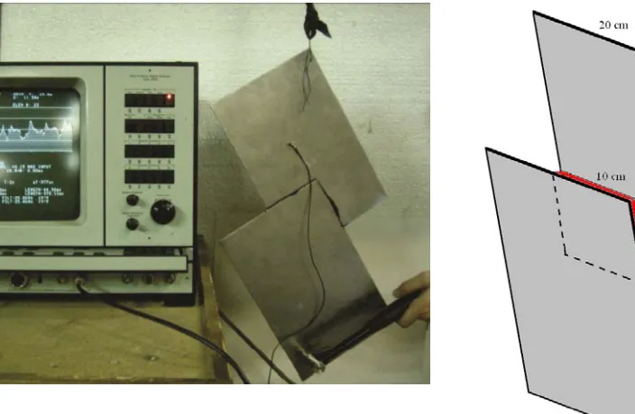
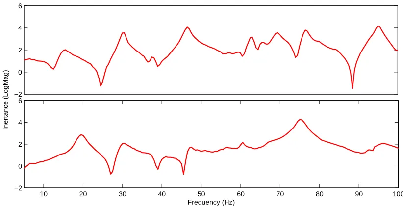
The test structure consists of two steel plates of thickness 1 mm bounded together with a layer of adhesive used in automotive industry with the thickness 3.5 mm. The industrial name of the adhesive layer is Sikaflex 252 with 1-C polyurethane chemical base. The material properties of the steel plates and adhesive are presented in Table 1. In order to avoid the effects of boundary conditions on natural frequencies, free-free boundary condition provided by suspending the structure using flexible strings is considered. The experimental test set-up is shown in Fig. (7). The hammer excitation technique is used to obtain the frequency response functions (FRFs) of the structure. The structure was excited by a B&K modal hammer and its dynamic response was measured by an accelerometer as shown in Fig. (7). The excitation force was measured by a force transducer provided in the hammer head. The measured force and response signals were transferred to a two channel B&K modal analyser in order to obtain the frequency response functions. Two measured FRFs are shown in Fig. (8). By using the measured FRFs, the natural frequencies are extracted. The first three natural frequencies are shown in Table 3.
First, a finite element model is constructed in MSC.NASTRAN® using relatively large number of elements. The adhesive layer is modelled by HEX8 solid elements. The mode shapes and the corresponding natural frequencies of the F.E. model are presented in Fig. (9). The MSC.NASTRAN® model and the experimental test results show that the identified three dominant natural frequencies-presented in Table 2 are correct and there is no missing mode between these three modes.
142
Fig. 8. Measured FRFs using the hammer test
Fig. 9. Mode shapes from the MSC.NASTRAN® model, a) 20.5 Hz, b) 34.29 Hz, c) 52.45 Hz
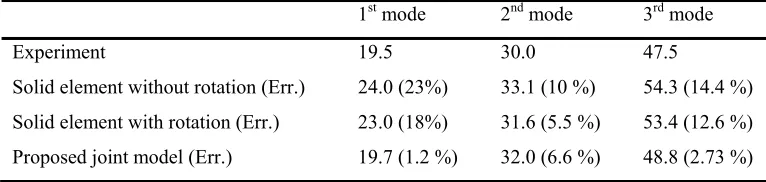
The convergence rate of the proposed joint element is compared to the conventional elements used in modelling the adhesive layer as described in the following. A finite element model is created employing three different elements for representing the adhesive layer: the 8-noded/3-DOF solid element, the solid element with Allman rotation degrees of freedom and the proposed joint element in this paper. In all cases, 16 elements are used for modelling the adhesive layer. The results of the F.E. models are compared with experimental results in Table 3.
−2 0 2 4 6
10 20 30 40 50 60 70 80 90 100
−2 0 2 4 6
Frequency (Hz)
143
Table 3. Comparison of experimental and F.E. natural frequencies
1st mode 2nd mode 3rd mode
Experiment 19.5 30.0 47.5
Solid element without rotation (Err.) 24.0 (23%) 33.1 (10 %) 54.3 (14.4 %) Solid element with rotation (Err.) 23.0 (18%) 31.6 (5.5 %) 53.4 (12.6 %) Proposed joint model (Err.) 19.7 (1.2 %) 32.0 (6.6 %) 48.8 (2.73 %)
The results presented in Table 3 indicate that the proposed joint model is capable to regenerate the experimental results with an acceptable accuracy.
Conclusion
Finite element modelling for adhesive joint was explored in this paper. To figure out the best model to represent dynamic behaviour of the adhesive layer, different types of elements were applied. It was found that the most accurate model is the joint element which is compatible with the plate element. The accuracy of the proposed joint model was validated by numerical and experimental case studies.
Appendix
Thin plate element shape functions are (
1
/
2
1
/
2
,
1
/
2
1
/
2
), ,/ ,
/a y b
x 4 / ) 2 1 )( 2 1 ( ) , (
1 x y
N 4 / ) 2 1 )( 2 1 ( ) , (
2 x y
N 4 / ) 2 1 )( 2 1 ( ) , (
3 x y
N 4 / ) 2 1 )( 2 1 ( ) , (
4 x y
N
+ -2 +2 -3/4 + - 3/4
2 -4 / 1 ) ,
( 3 3 3 3
1 x y
N ) 2 / 4 / 2 / 4 / 8 / 8 / 16 / 1 ( ) ,
( 2 3 2 3
2 x y b
N ) 2 / 4 / 2 / 4 / 8 / 8 / 16 / 1 ( ) ,
( 2 3 2 3
3 x y a
N
+ 2 -2 -3/4 - 3/4
2 4 / 1 ) ,
( 3 3 3 3
4 x y
N ) 2 / 4 / 2 / 4 / 8 / 8 / 16 / 1 ( ) ,
( 2 3 2 3
5 x y b
N ) 2 / 4 / 2 / 4 / 8 / 8 / 16 / 1 ( ) ,
( 2 3 2 3
6 x y a
N
- -2 +2 3/4 - 3/4 2 -4 / 1 ) ,
( 3 3 3 3
7 x y
N ) 2 / 4 / 2 / 4 / 8 / 8 / 16 / 1 ( ) ,
( 2 3 2 3
8 x y b
144 ) 2 / 4 / 2 / 4 / 8 / 8 / 16 / 1 ( ) ,
( 2 3 2 3
9 x y a
N
- 2 -2 3/4 + -3/4 2 4 / 1 ) ,
( 3 3 3 3
10 x y
N ) 2 / 4 / 2 / 4 / 8 / 8 / 16 / 1 ( ) ,
( 2 3 2 3
11 x y b
N ) 2 / 4 / 2 / 4 / 8 / 8 / 16 / 1 ( ) ,
( 2 3 2 3
12 x y a
N
References
[1] L.F.M. da Silva, P.J.C. das Neves, R.D. Adams, J.K. Spelt, Analytical models of adhesively bonded joints—Part I: Literature survey, International Journal of Adhesion and Adhesives, 29 (2009) 319-330.
[2] L.F.M. da Silva, P.J.C. das Neves, R.D. Adams, A. Wang, J.K. Spelt, Analytical models of adhesively bonded joints—Part II: Comparative study, International Journal of Adhesion and Adhesives, 29 (2009) 331-341.
[3] S. El-Sayed, S. Sridharan, Predicting and tracking interlaminar crack growth in composites using a cohesive layer model, Composites Part B: Engineering, 32 (2001) 545-553.
[4] M.A. McCarthy, C.G. Harte, J.F.M. Wiggenraad, A.L.P.J. Michielsen, D. Kohlgrueber, A. Kamoulakos, Finite element modelling of crash response of composite aerospace sub-floor structures, Computational Mechanics, 26 (2000) 250-258.
[5] A. Kaya, M.S. Tekelioğlu, F. Findik, Effects of various parameters on dynamic characteristics in adhesively bonded joints, Materials Letters, 58 (2004) 3451-3456.
[6] X. He, Finite element analysis of torsional free vibration of adhesively bonded single-lap joints, International Journal of Adhesion and Adhesives, 48 (2014) 59-66.
[7] A.S. Nobari, K. Jahani, Identification of damping characteristic of a structural adhesive by extended modal based direct model updating method, Experimental mechanics, 49 (2009) 785-798.
[8] K. Jahani, A.S. Nobari, Identification of dynamic (Young’s and shear) moduli of a structural adhesive using modal based direct model updating method, Experimental Mechanics, 48 (2008) 599-611.
[9] T. Naraghi, A.S. Nobari, Identification of the dynamic characteristics of a viscoelastic, nonlinear adhesive joint, Journal of Sound and Vibration, 352 (2015) 92-102.
[10] X. He, S.O. Oyadiji, Influence of adhesive characteristics on the transverse free vibration of single lap-jointed cantilevered beams, Journal of Materials Processing Technology, 119 (2001) 366-373.
[11] Y. Du, L. Shi, Effect of vibration fatigue on modal properties of single lap adhesive joints, International Journal of Adhesion and Adhesives, 53 (2014) 72-79.
[12] E. Nwankwo, A.S. Fallah, L.A. Louca, An investigation of interfacial stresses in adhesively-bonded single lap joints subject to transverse pulse loading, Journal of Sound and Vibration, 332 (2013) 1843-1858.
[13] D.J. Allman, A compatible triangular element including vertex rotations for plane elasticity analysis, Computers & Structures, 19 (1984) 1-8.
[14] E. Abdullah, J.F. Ferrero, J.J. Barrau, J.B. Mouillet, Development of a new finite element for composite delamination analysis, Composites Science and Technology, 67 (2007) 2208-2218.
[15] K.Y. Sze, A. Ghali, A hybrid brick element with rotational degrees of freedom, Computational Mechanics, 12 (1993) 147-163.
[16] R.H. Macneal, R.L. Harder, A refined four-noded membrane element with rotational degrees of freedom, Computers & Structures, 28 (1988) 75-84.
[17] S.M. Yunus, T.P. Pawlak, R.D. Cook, Solid elements with rotational degrees of freedom: Part 1—hexahedron elements, International Journal for Numerical Methods in Engineering, 31 (1991) 573-592.
[18] R.D. Cook, On the Allman triangle and a related quadrilateral element, Computers & Structures, 22 (1986) 1065-1067.