Truncated Software Reliability Growth Model Based on Linear Failure Rate Model - Release Time Policy

(1)

Truncated Software Reliability Growth Model Based on

Linear Failure Rate Model - Release Time Policy

B. Vara Prasad Rao1,*_{, K. Gangadhara Rao}2

1_{Department of Computer Science & Engineering, R.V.R & J.C College of Engineering, Chowdavaram, Guntur, Andhra Pradesh, India} 2_{Department of Computer Science & Engineering, Acharya Nagarjuna University, Guntur, Andhra Pradesh, India}

Abstract

A Non Homogenous Poisson Process (NHPP) with its mean value function generated by the cumulative distribution function of linear failure rate distribution is considered. We consider some truncated time values and use them in the mean value function of NHPP. The variation of the original mean value function and the mean value function at the truncated time is considered. A decision is taken to stop testing the software based on the difference between the mean value function and the mean value function at the truncated time. Truncated reliability aspects are discussed using four data sets.

Keywords

SRGM, RELEASE TIME

1. Introduction

In the theory of probability, F(t) is called the cumulative distribution function (CDF) of a continuous non-negative valued random variable. Thus an NHPP designed to study the failure process of a software can be constructed as a Poisson process with mean value function based on the cumulative distribution function of a continuous positive valued random variable. If a software system when put to use fails with probability F(t) before time t, if 'a' stands for the unknown eventual number of failures that it is likely to experience, then the average number of failures expected to be experienced before time t is a.F(t). Hence a.F(t) can be taken as the mean value function of an NHPP. We know that the cumulative distribution function (cdf) of the linear failure rate distribution is given by

𝐹𝐹(𝑥𝑥) = 1− 𝑒𝑒�𝑎𝑎𝑥𝑥+ 𝑏𝑏2𝑥𝑥2�,𝑥𝑥> 0,𝑎𝑎> 0,𝑏𝑏> 0 (1.1) The NHPP with F(θ,x) as the mean value function is prepared by us as the SRGM for our present study.

𝐹𝐹(𝜃𝜃,𝑥𝑥) =𝜃𝜃 �1− 𝑒𝑒�𝑎𝑎𝑥𝑥+ 𝑏𝑏₂𝑥𝑥2�_�_,_𝑥𝑥_{> 0,}_𝑎𝑎_{> 0,}_𝑏𝑏_{> 0,}_𝜃𝜃_{> 0}_(1.2)

Cumulative distribution functions of positive valued random variables play an important role in the development of software reliability growth models through non-homogenous Poisson process (NHPP) in Pham (2000) [2]. The notion of NHPP with cumulative distribution

function of LFRD along with the concept of truncation is

* Corresponding author:

[email protected] (B. Vara Prasad Rao) Published online at http://journal.sapub.org/safety

used in this work in an admissible way to decide the point of truncation on one hand and the optimal release time of the software product in a di erent sense. The suggested procedure is illustrated for four different data sets also. The rest of the paper is organized as follows. Evaluation of the mean value function by moment type method of estimation of statistical science given by Kantam et al. (2014) [1] is briefly presented in section 2. Our suggested procedure for the estimated mean value function to a hypothetical data set is described by section 3. The illustration of the results of our procedure for live data sets is presented in section 4. Summary and conclusions are given in section 5.

2. Moment Type Method of Estimation

The parameters of the mean value function generated by NHPP using LFRD model requires estimation because they are generally unknown. The most frequently used classical method of estimation is the well known Maximum likelihood method. However for LFRD model this method does not yield analytical solutions. As an alternative Kantam et al. (2014) [1] suggested a simpler, efficient ready to use method called moment type method of estimation and provided auxiliary tables for immediate use overcoming numerical iterative procedures. For the sake of theoretical justication the moment type method of estimation is briefly in this section. This method applied to any data gives the estimation of parameters the mean value function which is essential for a suggested procedure described in section 3.

(2)

distributions a com-bination of exponential distribution which is CFR model and Rayleigh which is IFR model is used through hazard function to get a model called LFRD whose hazard function is a perfectly increasing straight line of the form y=a+bx. Such a distribution is proved to be having a number of important applications in survival analysis, a proxy concept to reliability theory with a view to model software failure data with LFRD. We consider the pdf.

The probability density function (pdf) of Linear Failure Rate Distribution is given by

𝑓𝑓(𝑥𝑥) = (𝑎𝑎+𝑏𝑏𝑥𝑥) 𝑒𝑒�𝑎𝑎𝑥𝑥+ 2𝑏𝑏𝑥𝑥2�,𝑥𝑥> 0,𝑎𝑎> 0,𝑏𝑏> 0 (2.1) Its cumulative distribution function (cdf) is

𝐹𝐹(𝑥𝑥) = 1− 𝑒𝑒�𝑎𝑎𝑥𝑥+ 𝑏𝑏2𝑥𝑥2�,𝑥𝑥> 0,𝑎𝑎> 0,𝑏𝑏> 0 (2.2) The NHPP with F(θ,x) as the mean value function is prepared by us as the SRGM for our present study.

𝐹𝐹(𝜃𝜃,𝑥𝑥) =𝜃𝜃 �1− 𝑒𝑒�𝑎𝑎𝑥𝑥+ 𝑏𝑏2𝑥𝑥2��,𝑥𝑥> 0,𝑎𝑎> 0,𝑏𝑏> 0,𝜃𝜃> 0(2.3)

Thus our proposed SRGM contains 3 parameters namely

θ, a, b where θ stands for the unknown number of faults

latent in the software. It is also the limiting value of the

mean value function as t∞. For any general NHPP

representing as SRGM the software reliability is given by 𝑅𝑅�𝑥𝑥 𝑡𝑡� �=𝑃𝑃{𝑁𝑁(𝑡𝑡+𝑥𝑥)− 𝑁𝑁(𝑡𝑡) = 0} =𝑒𝑒−[𝑚𝑚(𝑡𝑡+𝑥𝑥)−𝑚𝑚(𝑡𝑡)]_(2.4) which is the probability of zero failures between the time t to t+x where t is the execution time of the software during which testing was done and x is additional time period upto which the user wants the software to function failure free. The quality of the software is based on the magnitude of the software reliability. We can know it only if the parameters of SRGM are known and t,x are specified. But generally, the parameters remain unknown and need to be estimated with the help of software failure data. Usually, the parameters will be estimated using the classical M.L. method. The loglikelihood equations to get the MLEs of the parameter after simplification for LFRD generated SRGM are:

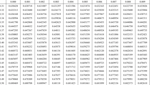
Table 1. Auxiliary Table of CV for a given θ

(3)

0.000 0.001 0.002 0.003 0.004 0.005 0.006 0.007 0.008 0.009 0.31 0.630428 0.630718 0.631007 0.631297 0.631586 0.631874 0.632163 0.632451 0.632739 0.633026 0.32 0.633313 0.633600 0.633887 0.634173 0.634459 0.634745 0.635030 0.635315 0.635600 0.635884 0.33 0.636168 0.636452 0.636736 0.637019 0.637302 0.637585 0.637867 0.638149 0.638431 0.638713 0.34 0.638994 0.639275 0.639555 0.639836 0.640116 0.640395 0.640675 0.640954 0.641233 0.641511 0.35 0.641790 0.642068 0.642345 0.642623 0.642900 0.643177 0.643453 0.643730 0.644006 0.644281 0.36 0.644557 0.644832 0.645107 0.64538 0.645655 0.645929 0.646203 0.646476 0.646750 0.647022 0.37 0.647295 0.647567 0.647839 0.64811 0.648382 0.648654 0.648924 0.649195 0.649465 0.649735 0.38 0.650005 0.650275 0.650544 0.65081 0.651081 0.651350 0.651618 0.651886 0.652153 0.652421 0.39 0.652688 0.652954 0.653221 0.65348 0.653753 0.654018 0.654284 0.654549 0.654814 0.655078 0.40 0.655343 0.655607 0.655870 0.65613 0.656397 0.656660 0.656923 0.657185 0.657447 0.657709 0.41 0.657971 0.658232 0.658493 0.65875 0.659014 0.659275 0.659535 0.659794 0.660054 0.660313 0.42 0.660572 0.660831 0.661089 0.66134 0.661605 0.661863 0.662120 0.662378 0.662634 0.662891 0.43 0.663147 0.663403 0.663659 0.66391 0.664170 0.664425 0.664680 0.664935 0.665189 0.665443 0.44 0.665697 0.665950 0.666204 0.66645 0.666709 0.666962 0.667214 0.667466 0.667718 0.667969 0.45 0.668221 0.668472 0.668722 0.66897 0.669223 0.669473 0.669723 0.669972 0.670222 0.670471 0.46 0.670719 0.670968 0.671216 0.67146 0.671712 0.671959 0.672207 0.672454 0.672700 0.672947 0.47 0.673193 0.673439 0.673685 0.67393 0.674176 0.674421 0.674666 0.674910 0.675155 0.675399 0.48 0.675643 0.675886 0.676130 0.67637 0.676616 0.676858 0.677101 0.677343 0.677585 0.677826 0.49 0.678068 0.678309 0.678550 0.67879 0.679031 0.679272 0.679512 0.679751 0.679991 0.680230 0.50 0.680469 0.680708 0.680947 0.68118 0.681423 0.681661 0.681899 0.682136 0.682373 0.682610

�𝑡𝑡𝑖𝑖𝑒𝑒−𝑎𝑎𝑡𝑡𝑖𝑖−𝑏𝑏2𝑡𝑡𝑖𝑖 2

− 𝑡𝑡𝑖𝑖−1𝑒𝑒−𝑎𝑎𝑡𝑡𝑖𝑖−1−𝑏𝑏2𝑡𝑡𝑖𝑖−1 2

𝑒𝑒−𝑎𝑎𝑡𝑡𝑖𝑖−1−𝑏𝑏₂𝑡𝑡𝑖𝑖−21− 𝑒𝑒−𝑎𝑎𝑡𝑡𝑖𝑖−𝑏𝑏₂𝑡𝑡𝑖𝑖2

(𝑦𝑦𝑖𝑖− 𝑦𝑦𝑖𝑖−1)

−𝜃𝜃𝑡𝑡𝑛𝑛e−𝑎𝑎𝑡𝑡𝑛𝑛+

𝑏𝑏

2𝑡𝑡𝑛𝑛2 = 0 (2.5)

�𝑡𝑡𝑖𝑖2𝑒𝑒−𝑎𝑎𝑡𝑡𝑖𝑖−𝑏𝑏2𝑡𝑡𝑖𝑖 2

− 𝑡𝑡𝑖𝑖−21𝑒𝑒−𝑎𝑎𝑡𝑡𝑖𝑖−1−𝑏𝑏2𝑡𝑡𝑖𝑖−1 2

𝑒𝑒−𝑎𝑎𝑡𝑡𝑖𝑖−1−𝑏𝑏₂𝑡𝑡𝑖𝑖−21_{− 𝑒𝑒}−𝑎𝑎𝑡𝑡𝑖𝑖−𝑏𝑏₂𝑡𝑡𝑖𝑖2

(𝑦𝑦𝑖𝑖− 𝑦𝑦𝑖𝑖−1)

−𝜃𝜃𝑡𝑡𝑛𝑛2e−𝑎𝑎𝑡𝑡𝑛𝑛+

𝑏𝑏

2𝑡𝑡𝑛𝑛2 = 0 (2.6)

𝜃𝜃 = yn

1−e−𝑎𝑎𝑡𝑡𝑛𝑛+ 𝑏𝑏2𝑡𝑡𝑛𝑛2

(2.7)

In view of the complicated nature to get the solutions of loglikelihood equations, we resort to moment type of estimation of the parameters as provided in kantam et al (2014) [1]. For a ready reference this method is presented below briefly:

The Mean, Variance and coefficient of variation (CV) of a reparameterised LFRD are respectively

µ =�2_𝑏𝑏𝜋𝜋 𝑒𝑒�𝑎𝑎

2 2𝑏𝑏��1−𝜙𝜙�

𝑎𝑎

√𝑏𝑏�� (2.8)

𝜎𝜎2₌2

𝑏𝑏(1− 𝑎𝑎µ)−µ2 (2.9)

𝐶𝐶𝐶𝐶=

⎝ ⎜

⎛2𝑏𝑏�1−√2𝜋𝜋𝜃𝜃e θ2

2�1−𝜙𝜙(𝜃𝜃)�−𝜋𝜋�𝑒𝑒𝜃𝜃 2 2�

2

�1−𝜙𝜙(𝜃𝜃)�2�

2𝜋𝜋 𝑏𝑏�𝑒𝑒

𝜃𝜃2 2�

2

�1−𝜙𝜙(𝜃𝜃)�2

⎠ ⎟ ⎞ 2

(2.10)

where ϕ(θ) is cumulative distribution function of standard

normal distribution. It can be seen that from equation (2.10) that there is a one-one correspondence between the

population CV and θ of reparameterised LFRD. This

motivates us to develop an auxiliary table between various hypothetical values of and CV expressed by equation (2.10). In fact the RHS of equation (2.10) is evaluated for various values of =0(0.001)0.5, so that for any live value of coefficient of variation (CV) one can get back the

corresponding θ, with interpolation if necessary. A part of

the values corresponding to =0(0.001)0.5 is listed in the table 1. The remaining values are available with the authors.

3. Procedure to Determine Truncated

Point

It is well known that a typical software failure data set shall be of the form (ti,yi), i=1,2,..,k. where ti is the time and

yi is the number of failures experienced by a software up to

time ti, also t1 < t2 < ::: < tk. In our procedure we take the

first two time incidents initially say (t1,t2) and define a

hypothetical truncated time for this subset as something

more than t2 say T1. Using the time point (t1,t2) the

parameters of the mean value function are estimated by the method described in section 2. These estimates would give

the estimated values of the mean value function at (t1; t2;

T1).The absolute difference of |m(t2) - m(T1)| is noted down

say A1.

The data is now supplemented by the next two time

(4)

points t1 < t2 < t3 < t4 in a moving manner. For this supplemented data set another hypothetical truncation time

say T2 typically more than t4 is taken. As described above

the parameters are estimated using t1 to t4 and the absolute

difference between |m(t4) - m(T2)| say A2 is noted down. This procedure is repeated each time supplementing the

data by the successive pairs of time incidents ti, ti+1 and

estimating the corresponding absolute difference Al at the ith

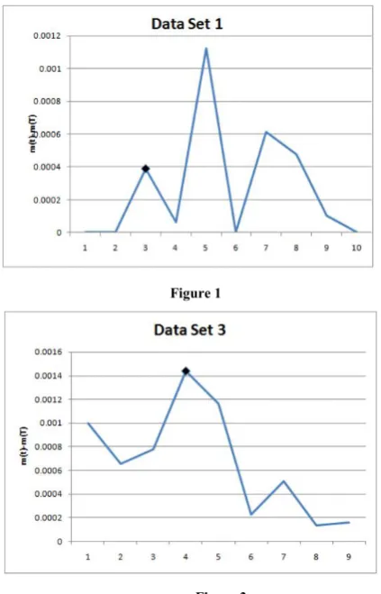
time till all the time points up to tk are exhausted. For a

given data set the graph of Al against l (l=1,2,...) shows a

trend of falling down and raising at a particular l where the

direction is changed is identi ed and the maximum ti of the

time points used at that stage is recommended as the suitable point of truncation. That point may be taken as the optimum release time of the software product and also the termination time at the software testing. This procedure is

applied to four data sets as illustration and is given in section 4.

4. Illustration

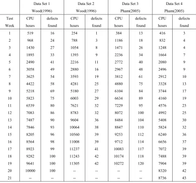
Four different data sets published in Wood (1996) [3] and Pham (2005) [4] are considered for illustration of the above procedure to determine the truncation point. The last row

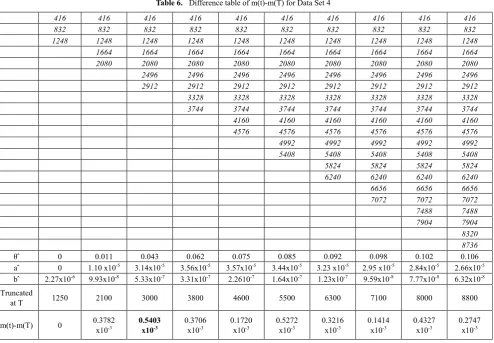
presented in the table of each data set indicates Al values.

The place at l where the trend of Al changes its direction is

shown in bold type. At that place in the column of tis the

largest ti is recommended as truncation time also marked in

bold type which in our proposal as the optimal release time / stoppage rule of the software testing.

Table 2. Data Sets

Data Set 1 Data Set 2 Data Set 3 Data Set 4 Wood(1996) Wood(1996) Pham(2005) Pham(2005) Test CPU defects CPU defects CPU defects CPU defects Week hours found hours found hours found hours found

1 519 16 254 1 384 13 416 3

2 968 24 788 3 1186 18 832 4

3 1430 27 1054 8 1471 26 1248 4

4 1893 33 1393 9 2236 34 1664 7

5 2490 41 2216 11 2772 40 2080 9 6 3058 49 2880 16 2967 48 2496 9 7 3625 54 3593 19 3812 61 2912 10 8 4422 58 4281 25 4880 75 3328 13 9 5218 69 5180 27 6104 84 3744 17 10 5823 75 6003 29 6634 89 4160 19 11 6539 80 7621 32 7229 95 4576 23 12 7083 86 8783 32 8072 100 4992 25 13 7487 90 9604 36 8484 104 5408 30 14 7846 93 10064 38 8847 110 5824 32 15 8205 96 10560 39 9253 112 6240 36 16 8564 98 11008 39 9712 114 6656 37 17 8923 99 11237 41 10083 117 7072 39 18 9282 100 11243 42 10174 118 7488 39 19 9641 100 11305 42 10272 120 7904 39 20 10000 100 -- -- -- -- 8320 42

(5)

Table 3. Difference table of m(t)-m(T) for Data Set 1

519 519 519 519 519 519 519 519 519 519

968 968 968 968 968 968 968 968 968 968

1430 1430 1430 1430 1430 1430 1430 1430 1430

1893 1893 1893 1893 1893 1893 1893 1893 1893

2490 2490 2490 2490 2490 2490 2490 2490

3058 3058 3058 3058 3058 3058 3058 3058

3625 3625 3625 3625 3625 3625 3625

4422 4422 4422 4422 4422 4422 4422

5218 5218 5218 5218 5218 5218

5823 5823 5823 5823 5823 5823

6539 6539 6539 6539 6539

7083 7083 7083 7083 7083

7487 7487 7487 7487

7846 7846 7846 7846

8205 8205 8205

8564 8564 8564

8923 8923

9282 9282

9641 10000

θ ̂ 0 0 0.068 0.169 0.258 0.277 0.23 0.173 0.123 0.084 a ̂ 0 0 0.4712 _x10-4 0.8152 _x10-4 0.9113 _x10-4 0.7913 _x10-4 0.5805 _x10-4 0.2699 _x10-4 0.2708 _x10-4 0.1089 _x10-4

b ̂ 0.2842 _x10-5 0.1086 _x10-5 0.4803 _x10-6 0.2327 _x10-6 0.1248 _x10-6 0.8816 _x10-5 0.6870 _x10-7 0.2440 _x10-7 0.4850 _x10-7 0.1680 _x10-7

Truncated

at T 1000 1900 3100 4500 5900 7100 7900 8600 9300 10000 m(t)-m(T) 0.0000 0.0000 0.3868 _x10-3 0.6358 _x10-4 0.1122 _x10-2 0.000 0.6110 _x10-3 0.4754 _x10-3 0.1013 _x10-3 0.0000

254 254 254 254 254 254 254 254 254

788 788 788 788 788 788 788 788 788

1054 1054 1054 1054 1054 1054 1054 1054 1054

1393 1393 1393 1393 1393 1393 1393 1393

2216 2216 2216 2216 2216 2216 2216 2216

2880 2280 2280 2280 2280 2280 2280

3593 3593 3593 3593 3593 3593 3593

4281 4281 4281 4281 4281 4281

5180 5180 5180 5180 5180 5180

6003 6003 6003 6003 6003

7621 7621 7621 7621 7621

8783 8783 8783 8783

9604 9604 9604 9604

10064 10064 10064

10560 10560 10560

11008 11008

11237 11237

11243 11305

θ ̂ 0.160 0.346 0.544 0.608 0.778 0.882 0.737 0.573 0.413 a ̂ 0.2537x10-3 _0.2961x10-3_0.2677x10-3 _0.2092x10-3 _0.1816x10-3 _0.1497x10-3 _0.1139x10-3 _0.8476x10-4 _0.6200x10-4

b ̂ 0.2515x10-4 _0.7326x10-6 _0.2423x10-6 _0.1184x10-6 _0.5450x10-7 _0.2880x10-7 _0.2390x10-7 _0.2190x10-7 _0.2250x10-7

Truncated

(6)

384 384 384 384 384 384 384 384 384

1186 1186 1186 1186 1186 1186 1186 1186 1186

1471 1471 1471 1471 1471 1471 1471 1471 1471

2236 2236 22363 2236 2236 2236 2236 2236

2216 2216 2216 2216 2216 2216 2216 2216

2772 2772 2772 2772 2772 2772 2772

2967 2967 2967 2967 2967 2967 2967

3812 3812 3812 3812 3812 3812

4880 4880 4880 4880 4880 4880

6104 6104 6104 6104 6104

6634 6634 6634 6634 6634

7229 7229 7229 7229

8484 8484 8484 8484

8847 8847 8847

9253 9253 9253

9712 9712

10083 10083

10174 10272

θ ̂ 0.084 0.141 0.085 0.336 0.359 0.332 0.256 0.192 0.121 a ̂ 0.9759x10-4 _0.9853x10-4 _0.4726x10-4 _0.1152x10-3 _0.9666x10-4 _0.7537x10-3 _0.5370x10-4 _0.3761x10-4 _0.2291x10-4

b ̂ 0.1349x10-5 _0.4884x10-6 _0.3090x10-6 _0.1176x10-5 _0.7250x10-7 _0.5150x10-7 _0.4401x10-7 _0.3840x10-7 _0.3590x10-7

Truncated

at T 1500 2800 3900 6200 7300 8500 9300 10100 10300 m(t)-m(T) 0.9992x10-3 _0.6578x10-3_0.7765x10-3_0.1438x10-2 _0.1162x10-2_0.2242x10-3_0.5085x10-3_0.1343x10-3_0.1571x10-3

416 416 416 416 416 416 416 416 416 416

832 832 832 832 832 832 832 832 832 832

1248 1248 1248 1248 1248 1248 1248 1248 1248 1248

1664 1664 1664 1664 1664 1664 1664 1664 1664

2080 2080 2080 2080 2080 2080 2080 2080 2080

2496 2496 2496 2496 2496 2496 2496 2496

2912 2912 2912 2912 2912 2912 2912 2912

3328 3328 3328 3328 3328 3328 3328

3744 3744 3744 3744 3744 3744 3744

4160 4160 4160 4160 4160 4160

4576 4576 4576 4576 4576 4576

4992 4992 4992 4992 4992

5408 5408 5408 5408 5408

5824 5824 5824 5824

6240 6240 6240 6240

6656 6656 6656

7072 7072 7072

7488 7488

7904 7904

8320 8736

θ ̂ 0 0.011 0.043 0.062 0.075 0.085 0.092 0.098 0.102 0.106 a ̂ 0 1.10 x10-5 _3.14x10-5 _3.56x10-5 _3.57x10-5 _3.44x10-5 _{3.23 x10}-5 _{2.95 x10}-5 _2.84x10-5 _2.66x10-5

b ̂ 2.27x10-6 _9.93x10-8 _5.33x10-7 _3.31x10-7 _2.2610-7 _1.64x10-7 _1.23x10-7 _9.59x10-8 _7.77x10-8 _6.32x10-8

Truncated

at T 1250 2100 3000 3800 4600 5500 6300 7100 8000 8800

(7)

Graphs indicating release time based on the mean value function

Figure 1 Figure 2

Figure 3 Figure 4

5. Summary & Conclusions

In software testing processes testing time is a key aspect. It is desirable to suggest a time point where testing is to be terminated and the product is to be released. In such situations a admissible stoppage rule is necessary to save the time aspect. The notion of truncation is used in this work to suggest optimal stoppage rule for a software product assuming that the failure phenomenon of the product is described by our NHPP with LFRD cdf as its mean value function. The method we suggested is simpler in mathematics without sacri cing its precision and can be readily used by practitioners to arrive at the stopping rule of the experiment.

REFERENCES

[1] Kantam. R. R. L., Priya. M. Ch., and Ravikumar. M. S Moment type estimation in linear failure rate distribution. IAPQR Transactions, 39(1):87-97, 2014.

[2] Pham. H. Software Reliability. Springer-Verlag, 2000. [3] Wood. A. P. Predicting software reliability. IEEE Computer,

11:69-77, 1996.