A New Technique of Room Access Security based Brain Computer Interface

ISSN: 1942-9703 / CC BY-NC-ND

Abstract— Vissim is a simulation software that has many uses. With its complete features, simulation of traffic conditions can be done to represent real world conditions. However, the limitations of Vissim's algorithm become an obstacle for developing the right traffic scheme. In order to implement custom algorithms, users need to bridge Vissim with applications that can process complex mathematical equation. It can be done using one of Vissim's feature called Vissim-COM interface. The use of Vissim-COM is crucial when users have to include custom algorithms that are not available on the Vissim GUI. Unfortunately, the use of Vissim-COM is a very rare thing done by the traffic engineer. Therefore, clear explanation on how to use Vissim-COM interface has also become a rare thing to find. This paper will provide some explanation on how to use Vissim-COM, including case studies of traffic control using custom algorithm to test the Vissim-Matlab interaction. This case study will use the traffic condition of Simpang Dago, Bandung. The use of custom algorithm was very effective to reduce the queue length, the custom algorithm result showed that the queue length of all 4 links were between 18-36 meters. Meanwhile, the queue length of the same links using traditional fixed time control were between 11-173 meters.

Index Terms— Vissim, Matlab, Traffic Engineering, Simulation, COM Interface

I. INTRODUCTION

RAFFIC management is one way to provide a better traffic condition. Good traffic management always starts by designing the right scenario. However, the implementation of this traffic scenario is sometimes constrained by the difficulty of conducting real traffic engineering. Traffic engineering that directly applied on the streets often have disadvantages such as: the need for socialization to road users, limited time available, large costs, and the risk of failure that can lead to severe congestion.

A way that can overcome these shortcomings is by doing the engineering in the simulation software. Simulation software can provide an approach to the various conditions that occur in the streets. There are many kinds of simulation software that can be used according to user needs. Based on network size, traffic analysis is divided into macroscopic,

Manuscript received June 10, 2018.

S. A. Ramadhan is with the Department of Instrumentation and Control Engineering Institut Teknologi Bandung, Indonesia (phone: +62 822 9920 6605; e-mail: [email protected]).

E. Joelianto, is with the Department of Instrumentation and Control Engineering Institut Teknologi Bandung, Indonesia (Corresponding author e-mail: [email protected]).

H. Y. Sutarto is with the East Continent Research Center, Indonesia (e-mail: [email protected]).

mesoscopic, and microscopic levels. Microscopic analysis is the most accurate level of analysis because it takes into consideration many small factors such as vehicle volume, turning ratio, speed distribution, and driving behavior.

There are several traffic simulation softwares that can be used, such as Vissim or SUMO. Airulla et. al. [1] performs the implementation of Mix-Max algorithm using MPC on the Surabaya traffic network using SUMO. But the use of SUMO has its own complexity. Because it is a Linux-based program, the whole process of its use must be done manually by writing the program. Vissim offers ease of use over SUMO, because Vissim already has its own user interface, so users do not need to write the program manually.

PTV Vision is a company that develops various traffic simulation software. There are various types of software provided by PTV Vision ranging from macroscopic to microscopic level. PTV Vissim is one of the software developed by PTV Vision, which runs traffic simulation at microscopic level.

PTV Vissim is the leading microscopic simulation program for modeling multimodal transport operations and belongs to the Vision Traffic Suite software. Realistic and accurate in every detail, Vissim creates the best conditions for people to test different traffic scenarios before their realization. Vissim is now being used worldwide by the public sector, consulting firms and universities. [2]

Vissim has various features, such as traffic flow modeling, traffic light engineering, vehicle queue length analysis, pedestrian simulation, and also script-based modeling. Script-based modeling is one of Vissim's features that is very useful in the development of traffic control algorithms. Through COM (Component Object Model) Interface, users can connect Vissim with various programming language applications such as C ++, Java, Phyton, Matlab, VBA, and others. Through this feature, users have the freedom to apply additional algorithms that are not available in Vissim.

There have been many studies that utilize Vissim to represent traffic conditions of real conditions [3] [4] [5] [6], but this research is still limited to the use of algorithms that is available within the Vissim GUI. The use of Vissim-COM is crucial when users have to include custom algorithms that are not available on the Vissim GUI. Knowledge on how to use Vissim-COM becomes something that must be mastered by researchers who want to develop algorithms with complex mathematical relationships.

However, the use of Vissim-COM is a very rare thing done

Simulation of Traffic Control Using

Vissim-COM Interface

Satria A. Ramadhan, Endra Joelianto, and Herman Y. Sutarto

by the traffic engineer. Seen from the lack of publications that utilize this feature. This is exacerbated by Vissim's policy, which has been limiting the help feature of Vissim-COM since the release of Vissim version 6.0.

There are not many publications that use the Vissim-COM feature as a way to connect Vissim with other programming application. Tettamanti et al [7] in 2012 published his study of the implementation of the MPC minimax algorithm utilizing the Vissim-Matlab relationship. Tettamanti also made several publications describing the mechanism of Vissim-COM's use in detail [8][9]. Another study using the Vissim-COM feature was performed by Maria Solomons who applied the backpressure algorithm to Vissim, using Matlab as a data processing application [10]. Although there are some papers that use Vissim-COM interaction, only publications from Tettamanti in 2015 [8][9] clearly address the stages in establishing the Vissim-COM connection.

In this paper, we will describe the steps carried out in the network modeling process and traffic control through Vissim-Matlab interaction, utilizing the COM interface feature. In section II will be discussed about the use of Vissim, the basics of Vissim COM programming, as well as the hierarchical structure contained in Vissim COM. Furthermore, in section III we will describe the traffic model design scheme in Vissim. Section IV will present a case study of traffic control using custom algorithm to test the Vissim-Matlab interaction

II. VISSIMANDCOMINTERFACE

A. Introduction to Vissim COM Interface

Vissim as a traffic simulation software already provides various features that make it a very complete simulation software. Through Vissim, users can conduct in-depth analysis of the junction geometry, planning infrastructure development, capacity management, development of traffic control systems, to simulate the development of public transport.

As a simulation software, Vissim also equips itself with various additional modules (APIs), which can help users integrate Vissim with various applications. One of the most useful APIs is the COM Interface. Some things that can be used through COM Interface are [2]:

• Preparation and postprocessing of data

• Efficiently controlling the sequence for the examination of scenarios

• Including control algorithms which you have defined

• Access to all network object attributes

Through COM Interface, users can run and access Vissim objects from other applications. COM can be used by using various programming environments and programming languages such as VBA in Ms. Excel, Visual C ++, Python, Delphi, and Matlab. Through the use of COM Interface, users can manipulate the various objects and attributes contained in Vissim dynamically.

COM Interface is an exclusive feature that can only be accessed on Vissim Full Version. Users must register Vissim as COM-server on the computer's operating system, so other applications can access COM objects.

B. Vissim-COM Object Model

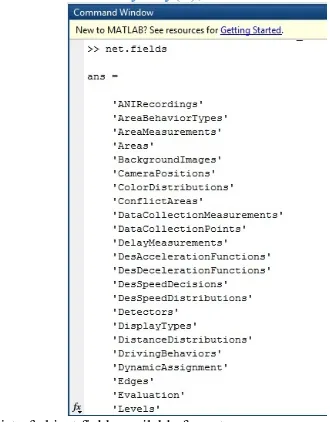
Vissim-COM implements a very strict hierarchical system in its use. Figure 1 shows the hierarchical system contained in Vissim-COM. As can be seen in the picture, the object in the hierarchy has a head called IVissim, which represents the Vissim object. There are 5 main objects under IVissim, which is ISimulation, INet, IGraphics, IPresentation, and IEvaluation.

ISimulation is an object used to access all attributes related to Vissim simulation parameters such as time period, step time, simulation speed, etc. INet is the largest object because it is used to access attributes related to the networks such as Link, Vehicle Input, Driving Behaviors, etc. IEvaluation is used to access evaluation parameters. IPresentation is used to access the 3D serving attribute. And the last object, IGraphics is used to access attributes related to the Vissim user interface.

All sub attributes under this object can be viewed in the offline help Vissim (Help \ COM Help), or can also be accessed through other applications by giving the command:

{Vissim-COM object name}.fields

ISSN: 1942-9703 / CC BY-NC-ND III. MODELLING THE NETWORK

In order to use COM Interface, users must first build a Vissim network model that will be used in COM Interface. This network will then become the basis for the use of COM Interface. The development of the required model includes the making of roads, route choices, determining the number of vehicles and their composition, to the control of green light allocation of each link.

In this paper, the application to be associated with Vissim is Matlab. The use of Matlab is based on the reasons for its ease of operation, the completeness of its features, and its ability to run specific algorithms.

In general, the steps in the process of using Vissim - Matlab interactions are shown in Figure 2.

Start

Generating overal traffic network through Vissim GUI

Connecting Vissim to Matlab

Implementing specific command/

algorithm for Vissim through

Matlab GUI

Running the simulation from

Matlab

End

Fig. 2. Flowchart of Vissim - Matlab interaction process

Connecting Vissim to Matlab

To connect Matlab with Vissim, create a new COM server on Matlab by entering the command:

vis=actxserver(‘VISSIM.vissim.{Vissim Version}’)

The use of vis in the above command is to define IVissim which will then be considered the head of the COM hierarchy. By giving actxserver command, Matlab will automatically connect with Vissim.

The user can then find various functions that can be done through COM interaction on the IVissim object by giving the command:

vis.methods

It will show a list of functions that can be used as in Figure 3:

Fig. 3. List of methods available for vis [4]

To find sub-objects under the IVissim object, the user can use the command:

vis.fields

The use of the command will bring up five main objects, that is INet, ISimulation, IEvaluation, IGraphics, and IPresentation.

Fig. 4. List of fields available for vis [4]

Loading the network

Network models that have been previously created, must be defined to be recognized by Matlab. When creating a network model, Vissim will generate two files with the .inpx extension, and .layx. By using the 'LoadNet' and 'LoadLayout' functions, define the location of the two files to be accessed by Matlab,

vis.LoadNet(‘{File Path}\{File Name}.inpx’) vis.Loadlayout(‘{File Path}\{File Name}.layx’)

If the definition process runs correctly, when the command is executed, automatically the layout that has been created will open in Vissim.

In order for the command-generation process in Matlab to run smoothly and well organized, it is recommended to define the 5 main objects of IVissim at the beginning by using the command:

sim=vis.Simulation; net=vis.Net; eval=vis.Evaluation; graph=vis.Graphics; pres=vis.Presentation;

Setting the simulation parameter

Through the use of Vissim-COM users have the freedom to obtain or enter values into objects available in Vissim via Matlab. The object's retrieval process can use the 'get' command, whereas the value setting uses the 'set' command. In order to access the desired attributes, the user must use the command 'AttValue'. Therefore, the command used to retrieve and enter data is:

sim.get(‘AttValue’, {‘attribute’};

sim.set(‘AttValue’, {‘attribute’}, {value};

simulated objects can be viewed in the offline help Vissim (Help \ COM Help), or by entering a command:

sim.fields

Users have the freedom to specify values of simulation parameters via Matlab, or directly from Vissim GUI.

Setting network attributes

The INet object is the object with the most sub-objects, because INet is the parent of all attributes associated with the model parameters. Through the INet object, the user can retrieve all the information of each link, provide the input of the number of vehicles, control all sensors and detectors, and make state changes to traffic lights. Just like ISimulation, users can also find a list of available INet objects through the command:

net.fields

Figure 5 shows the Matlab response when the user requests a list of objects under the INet object.

To access the sub-objects, the definitions in Matlab are done by writing the main object, followed by the desired sub-object. For example, to access VehicleInput, the command that is written is:

vehin=net.VehicleInput;

Sometimes, some specific objects are marked by a certain number code in the Vissim GUI, to access that specific object, the ItemByKey function can be used. For example, to access 'vehin' at a particular location, the user should pay attention to the number code corresponding to 'vehin' as desired. So the command is written:

vehin1=vehin.ItemByKey(1);

Fig. 5. List of object fields available for net

Most attributes under the INet object can only be accessed when the simulation has run, this is because Vissim needs to run the simulation to generate the required network related data. In the following section, a variety of controller algorithms will require various data generated on this INET object.

Running the simulation

Vissim has three ways to run simulations, RunContinuous, RunSingleStep, and RunMulti. RunContinuous will make the simulation run without pause, this way will make the simulation in Vissim running smoothly without pause.

However, the user can only access the simulation parameters after the simulation is completed. Instead, RunSingleStep will make the simulation truncated every time interval. In this way, the simulation display in Vissim will run disjointedly. However, users can access simulated data when simulation runs, because Vissim can provide parameter values during pause. RunSingleStep can be run with command 'for' on Matlab. So the command used to run the simulation would be:

for i=0:(period_time* time_step) sim.RunSingleStep;

end

Users can add various custom algorithms to the 'for' loop if they want to apply it during simulation.

The above stage is the last stage in the general process of creating COM syntax via Matlab. When the user runs the simulation via the 'Run' button in Matlab, the whole process will run automatically, until the user-defined simulation period is fulfilled.

IV. CASE STUDY

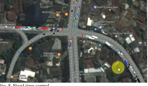
This case study uses the Simpang Dago network model, located in Bandung, Indonesia. In this case study, a traffic light controller algorithm will be implemented into the network model. Figure 6 shows the full network model. This intersection consists of 4 links, with each link is controlled using a traffic light. The algorithm will be applied into a 4 phase red light system. The custom algorithm will be compared with fixed time cycle control to see the difference of handling performance.

Fig. 6. Location of studied area

The model has 4 vehicle input locations: • North = 1000 Veh/hour

• East = 2500 Veh/hour • South = 1200 Veh/hour • West = 2500 Veh/hour

Simulation period is set to be 3600s, while the algorithm will be implemented every 30 second. Green time allocation for Fixed Time controller is 30 seconds for every links. The sequence of the green light on the Fixed Time controller is N-E-W-S.

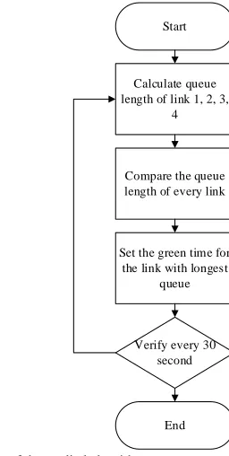
ISSN: 1942-9703 / CC BY-NC-ND Start

Calculate queue length of link 1, 2, 3,

4

Compare the queue length of every link

Set the green time for the link with longest

queue

Verify every 30 second

End

Fig. 7. Flowchart of the studied algorithm

As described in the previous chapter, the steps of command generation are connecting Vissim with Matlab, defining the layout location, defining the five main objects of IVissim, and assigning the simulation parameter values. Then the command is made:

vis=actxserver('Vissim.vissim.800'); --- access_path=pwd;

vis.LoadNet([access_path '\Dago.inpx']); vis.LoadLayout([access_path '\Dago.layx']); ---

sim=vis.Simulation; net=vis.Net; eval=vis.Evaluation; graph=vis.Graphics; pres=vis.Presentation;

--- period_time=3600;

time_step=3;

sim.set('AttValue', 'SimPeriod', period_time); sim.set('AttValue', 'SimRes', time_step);

Then, it is necessary to define the length of the queue sensor to be used. There are four queue sensors for each link, symbolized by SI, DA, DU, and DB. The QueueCounter sensor is under the INet object, so the command that is written is:

que=net.QueueCounters; SI=que.ItemByKey(1); DA=que.ItemByKey(2); DU=que.ItemByKey(3); DB=que.ItemByKey(4);

In order to control traffic lights, it is also necessary to define the traffic lights to be used, along with the signal groups that have been installed on each lamp. Signal group will only serve as a description that distinguishes one lamp with other lights. For the length of the fixed green light will be

determined by the algorithm. SignalControllers object is under the INet, and ItemByKey function will help select SignalController number 1. The Signal group (SGs) is under the SignalController sub-object number 1, where there will be 4 signal groups representing traffic lights on each link. The written command is:

scs=net.SignalControllers; sc=scs.ItemByKey(1); sgs=sc.SGs;

sg_1=sgs.ItemByKey (1); sg_2=sgs.ItemByKey (2); sg_3=sgs.ItemByKey (3); sg_4=sgs.ItemByKey (4);

Next is the implementation of the algorithm inside the 'for' loop. The algorithm is designed to set the green light priority every 30 seconds, so it is necessary to add the 'verify' command to the algorithm. To get the length of the queue recorded by the sensor, use the command 'get' and 'AttValue'. Then the command used is:

verify=30;

for i=0:(period_time* time_step) sim.RunSingleStep;

if rem(i/time_step,verify)==0

QL_B=SI.get('AttValue', 'QLen(Current,Last)') QL_U=DA.get('AttValue', 'QLen(Current,Last)') QL_T=DU.get('AttValue', 'QLen(Current,Last)') QL_S=DB.get('AttValue', 'QLen(Current,Last)') ---[ALGORITHM]--- end

end

Through the command above, we have obtained the queue length value of each link stored in the variable QL_B, QL_U, QL_T, QL_S. These four variables are compared every 30 seconds, and the link with the longest queue will be defined as Mx_Press. Thus, the algorithm used to complete the 'for' loop above is:

arr = [QL_B,QL_U,QL_T,QL_S];

arr_name = {'QL_B','QL_U','QL_T','QL_S'}; [maximum,ind]=max(arr);

Mx_Press=arr_name{ind} if Mx_Press == 'QL_U'

sg_1.set('AttValue', 'State', 3); sg_2.set('AttValue', 'State', 1);

sg_3.set('AttValue', 'State', 1); sg_4.set('AttValue', 'State', 1);

V. RESULTS

Based on the results of the above custom algorithm implementation, the result shows the difference of control performance between custom algorithm and fixed time control. Table 1 below shows the comparison of queue length in custom algorithm with fixed time. It can be seen in the table that the queue distribution on the custom algorithm is more evenly distributed on each link. Contrast with fixed time control that shows long queues only on west links and east links, which has the largest flow.

TABLEI

COMPARISON BETWEEN CUSTOM ALGORITHM AND FIXED TIME CONTROL

Custom Algorithm S E W N

Average Queue (m) 26.126 36.008 27.147 18.66 Stdev (m) 14.184 19.687 16.229 11.219 Max Queue (m) 65.16 123.34 82.89 52.85

Green Phase Count 20 37 38 21

Fixed Time S E W N

Average Queue (m) 16.142 170.87 173.32 11.247 Stdev (m) 8.383 38.135 36.868 6.968 Max Queue (m) 53.07 207.38 212.1 39.43

Green Phase Count 29 29 29 29

Other results obtained from the implementation of this algorithm is the number of green lights received by each link. The use of fixed time control will provide an even distribution of green light for all links, which is 29 times of green light in 3480 seconds operation. Meanwhile, the use of custom algorithm has set more green allocation on the west link and east link. This is the reason why custom algorithm provides more uniform distribution of queue length in custom algorithm.

Fig. 8. Fixed time control

Based on the visualization showed in Figure 8, it showed that the algorithm has successfully been applied in Vissim. From the Figure 8 we could see that the fixed time control gives bad result as the queue length reached its following intersection.

Different result showed in Figure 9, where the custom algorithm is applied. By using the same set data, and analyzed at the same time period, the algorithm showed a much better condition. Therefore, we could say that the algorithm that was written in Matlab has been successfully applied in Vissim

GUI. Later, the other intersection also will be controlled using the same algorithm, to provide global traffic control condition.

Fig. 9. Custom algorithm control

From the case study provided above, we can see that Matlab-Vissim interaction makes it easy for traffic algorithm developers to apply the algorithm they have created. Going forward, we hope more and more researchers started to use this Vissim-COM feature, so that more traffic control algorithms can be implemented in the real world.

VI. CONCLUSION

We have described the method of using Vissim-COM to connect Matlab with Vissim. Through the use of Vissim-COM, users can implement a variety of specific algorithms that are not available in Vissim-GUI Based on the given case study, it showed that Vissim-Matlab interaction has been successfully performed, with successful custom algorithms implemented in Vissim-GUI. Based on the simulation results, the use of custom algorithms has successfully lowered the queue length, and provides a more uniform distribution of queue length across all links.

Vissim is a simulation software that has many uses. With its complete features, simulation of traffic conditions can be done to near real world conditions. However, the limitations of Vissim's algorithm become an obstacle for developing the right traffic scheme. Through the use of COM Interface, these limitations can be overcome by connecting Vissim with a programming application that can implement specific algorithms. From the case studies presented in the paper, we could see that the Vissim-Matlab interaction has been successfully done. Vissim could recognize the custom algorithm that we implement from Matlab, through the use of Vissim-COM interface.

ACKNOWLEDGMENT

ISSN: 1942-9703 / CC BY-NC-ND Jalan dan Jembatan Bandung (PUSJATAN) on the permission

of using the Vissim Full Version.

REFERENCES

[1] E. Joelianto, H.Y. Sutarto, D.G. Airulla, and M. Zaky, "Design and Simulation of Traffic Light Control System at Two Intersections Using Max-Plus Model Predictive Control," To Appear International Journal of Artificial Intelligence (2019).

[2] PTV, “PTV Vissim 8 User Manual,” PTV Planung Transport Verkehr AG, Karlsruhe: PTV Planung Transport Verkehr AG., 2016.

[3] Fellendorf, Martin, "VISSIM: A microscopic simulation tool to evaluate actuated signal control including bus priority," 64th Institute of Transportation Engineers Annual Meeting, Springer, 1994.

[4] Park, Byungkyu, and J. Schneeberger, "Microscopic simulation model calibration and validation: case study of VISSIM simulation model for a coordinated actuated signal system," Transportation Research Record: Journal of the Transportation Research Board 1856, pp. 185-192, 2003. [5] Huang, Fei, et al., "Identifying if VISSIM simulation model and SSAM

provide reasonable estimates for field measured traffic conflicts at signalized intersections," Accident Analysis & Prevention, vol. 50, pp. 1014-1024, 2013.

[6] Mathew, Tom V., and Padmakumar Radhakrishnan, "Calibration of microsimulation models for nonlane-based heterogeneous traffic at signalized intersections," Journal of Urban Planning and Development,

vol. 136.1, pp. 59-66, 2010.

[7] Tettamanti, Tamás, and István Varga, "Development of road traffic control by using integrated VISSIM-MATLAB simulation environment," Periodica Polytechnica. Civil Engineering, vol. 56.1: 43. 2012.

[8] T. Tettamanti and M. T. Horvath, “A practical manual for Vissim COM programming in Matlab 2nd edition,” Budapest University of Technology and Economics, Budapest, rep., 2015.

[9] T. Tettamanti, “A practical manual for Vissim COM programming in Matlab 1st edition,” Budapest University of Technology and Economics, Budapest, rep., 2015.

[10] Salomons, A. Maria, and Andreas Hegyi. "Intersection Control and MFD Shape: Vehicle-Actuated versus Back-Pressure Control," IFAC-PapersOnLine 49.3 , pp. 153-158., 2016.

[11] PTV, “Introduction to the PTV Vissim 8 COM API.” PTV Planung Transport Verkehr AG, Karlsruhe: PTV Planung Transport Verkehr AG., 2016.

[12] Karaboga, Dervis. “An idea based on honey bee swarm for numerical optimization,” Vol. 200. Technical report-tr06”, Erciyes University, Engineering Faculty, Computer Engineering Department, 2005.

Satria A. Ramadhan received his B.S from the Department of Physics

Engineering, Universitas Gadjah Mada. Later, he finished his master degree at Institut Teknologi Bandung, majoring in Instrumentation and Control System. From 2014-2017, he was with Enerbi, a non-profit organization related to the renewable energy infrastructure development for rural areas. He joined Pusat Riset Energi, Ltd (https://rce.co.id/) in 2018, and is assigned as Junior Researcher to study about the implementations of traffic management system in Indonesia. His research interests are the implementations of control theories for traffic management system, and also its validation method such as Macroscopic Fundamental Diagram (MFD). He has also interest in community development, and also studies related to energy management system.

Endra Joelianto (M’01) received his B.Eng. degree in Engineering Physics

from Bandung Institute of Technology (ITB), Indonesia in 1990, and his Ph.D. degree in Engineering from The Australian National University (ANU), Australia in 2002.

He was a Research Assistant in the Instrumentation and Control Laboratory, Department of Engineering Physics, Bandung Institute Technology, Indonesia from 1990-1995. Since 1999, he has been with the Department of Engineering Physics, Bandung Institute of Technology, Bandung, Indonesia, where he is currently a Senior Lecturer. He has been a Senior Research Fellow in the Centre for Unmanned System Studies (CENTRUMS), Bandung Institute of Technology, Bandung, Indonesia since 2007, National Centre for Sustainable Transportation Technology and National Centre for Security and Defence at Bandung Institute of Technology,

Bandung, Indonesia since 2016. He was a Visiting Scholar in the Telecommunication and Information Technology Institute (TITR), University of Wollongong, NSW, Australia in February 2002. He was a Visiting Scholar in the Smart Robot Center, Department of Aerospace and Information Engineering, Konkuk University, Seoul, Korea in October 2010. His research interest includes hybrid control systems, discrete event systems, computational intelligence, robust control, unmanned systems, intelligent automation and industrial internet of things. He edited one book on intelligent unmanned systems (Springer) 2009, published one book on linear quadratic control (ITB-Press) 2017 and published more than 125 research papers.

Herman Y. Sutarto received a B.S and M.S. from the Department of