Assessment of dynamic linear and non-linear models on rainfall variations predicting of Iran

Assessment of dynamic linear and non-linear models on rainfall

variations predicting of Iran

Majid Javari

(College of Social Science, PayameNoorUniversity, Post Office Box 19395-3697, Tehran, Iran)

Abstract: The main research aims to detect the linear and nonlinear variability modeling in analyzing the variability patterns of

rainfall series. For rainfall linear and nonlinear variability modeling, the Autoregressive Integrated Moving Average (ARIMA) models and Autoregressive Conditional Heteroskedasticity (ARCH) family models have been used for predicting the monthly and annual rainfall series extracted from Islamic Republic of Iran Meteorological Office (IRIMO) between 1975 and 2014 within 140 stations in Iran. Several ARIMA and ARCH family (six models) models have been used and their validity has been confirmed by evaluating different accuracy indicators, using the hybrid model for the variability modeling. The analysis of ARIMA and Generalized Autoregressive Conditional Heteroskedasticity (GARCH) selective models indicated existence of random and non-random in the rainfall time series. The combination model of (1,0,0) and GARCH (1,1) is applied to the estimate and prediction of monthly rainfall. With careful valuation of the hybrid model, the ARIMA (1,0,0) and GARCH(1,1) is recognized as the significant acceptable model by determines of different accuracy indicators similar to mean squared error (77025.34); root mean squared error (277.53); mean absolute error (167.68); mean absolute percentage error (79.68); and Theil’s U coefficient (0.365). However, the results showed that the hybrid model, as a variability model is more efficient in forecasting the rainfall variability and underlying this model can be used as variability forecast model and chaos phenomena in Iran. In addition, a nonlinear model of ARCH family, especially GARCH (1,1) provided a quantitative-analytical method to distinguish between a particular random and non-random model for rainfall variability in Iran.

Keywords: linear models, Non-linear models, variability severity, and rainfall variability

Citation: Majid, J. 2017. Assessment of dynamic linear and non-linear models on rainfall variations predicting of Iran.

Agricultural Engineering International: CIGR Journal, 19(2): 224–240.

1 Introduction

The rainfall variability has important effects on the climate, and the variable patterns effects can be diverse at various temporal and spatial scales (Javari, 2017a). The concept of variability is widely being used in different subjects of climatology. There are various points of view about the concept of variability in climate and climatic elements (Javari, 2017d). In climatology, rainfall variability affects the regionalization of climate and hydrology, due to affecting drought and environmental conditions and the water supplies to economic development (Li et al., 2015; Narayanan et al., 2013)The

Received date: 2017-01-16 Accepted date: 2017-02-18 Biographies:Majid Javari, Assistant Professor of Climatology,

PayameNoor University, Tehran, Iran. Email: majid_javari@ yahoo.com. Tel: 09133285930, Fax: 32353666.

Generalized Autoregressive Conditional Heteroskedasticity (EGARCH), Glosten, Jagannathan and

Runkle (GJR) and Threshold Autoregressive Conditional Heteroskedasticity (TARCH), the preference of ARCH family models are the spatial distributions in the properties and patterns of rainfall, but these also can be nonlinear as they can response in very different rainfall variability (Javari, 2016) among stations (Gouriéroux, 2012; Hafner et al , 2015; Shimizu, 2014). Therefore, all climatic models need the variability forecasting. In the climate, some of the variability patterns are predictable (seasonality, trend and cyclic patterns), and some other is unpredictable (random patterns) (Javari, 2017b). Therefore, changes in monthly and seasonal variability patterns in rainfall amounts were being forecasted using ARCH family models as several nonlinear models to provide regionalization of rainfall in Iran. ARCH models have been applied in monthly, seasonal and annual rainfall to analyze and detect variability, the risk of thresholds climatic variations, evaluating the variation patterns, forecasting temporal variability confidence intervals and obtaining more efficient climatic patterns under the heteroskedasticity existence during the last 39 years (1975-2014) in the ARCH model, assume that the true climatic data is generating the process of continuous compounded returns, climatic variable has a quite unpredictable conditional mean and a temporal conditional variable variance. Temporal climatic variability theory expresses that a climatic element with a higher expected risk would affect a higher return on average. The relationship between expected effectiveness return and risk was suggested in an ARCH model (Engle et al., 1987). They presented the ARCH in mean, or ARCH-M, model where the conditional mean is an accurate pattern of the process conditional variance in variability as a function in ARCH. The ARCH-M model provided a new approach by which a temporal variable risk, and reliability analysis could be forecasted in the climate (Chambers et al., 1983; Souri, 2012). In this regard, the serial correlation in the analysis of climatic series is important. LeBaron (1992) noted a strong inverse relationship between variability and serial correlation for the model returns in the temporal analysis.

He presented the exponential autoregressive GARCH or EGARCH model in which the conditional mean is a non-linear pattern of the conditional variance for using the variability of climatic series. In this regard, the relationship between autocorrelation and variability, and predicting an inverse relationship between variability and autocorrelation in the analysis of climatic series is essential (Kim, 1989; Sentana et al., 1991). According to the multivariate ARCH models, the asymmetric modelling of the conditional variance as a forecast method is important. Therefore, the modelling of the conditional variance as a univariate GJR model is also used. The moment structure of the EGARCH model was investigated (He et al., 2002; Karanasos et al., 2003). Degiannakis (2008) showed that the TARCH model is able to statistically provide the temporal rainfall variability forecasts. One of the main aspects of ARIMA models is their ability to analyze the climatic changes in the climatic series and forecasting the climatic variability patterns (Javari, 2017c). In ARIMA models, the forecasted rainfall is calculated using a linear combination of the rainfall series in various stations. This study has investigated rainfall variability by implementation of ARCH and ARIMA models on the various types of rainfall series. The paper is organized as follows: we briefly introduced the ARCH and ARIMA methods to provide a description of our proposed method on precipitation in section 2. Section 3 presents the new model of rainfall variability in detail. The experimental results and conclusions are respectively presented in sections 4 and 5.

2 Materials and methods

2.1 Study areas and materials

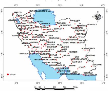
Iran lies between 25°3′-39°47′N in latitude and 44°5′-63°18′E in longitude in the southwestern of Asia (Figure 1). We obtained monthly, seasonal and annual rainfall data for all of Iran’s 140 stations from the IRIMO and 38746 rainfall points from has been extracted and processed the rainfall layers of Iran by using ArcGIS. Precipitation series of 140 stations and 38746 rainfall points in Iran were studied for the period of 1975-2014.

precipitation series of each station (Costa and Soares, 2009) by using SYSTAT, Eviews and Minitab softwares .

Figure 1 Selective stations in Iran

2.2 Methods

2.2.1 Definition the properties of models

In the use of time series models, there are important aspects of models that can be noted in this regard in order to forecast the models. This study summarizes the characteristics of the time series as follows:

ARCH Models: The ARCH models that are not constant at the Autoregressive Conditional variance. In the ARCH model, the autocorrelation in variability is expressed by the conditional variance of the error, which in the simplest case is dependent on the square error of the previous period.

GARCH Models: GARCH model is the generalized model of ARCH in which errors and variance are entered in the model with a lag.

GJR Model: GJR model is the simplest type of asymmetric GARCH model. In this model if the γ value is statistically not significant, it means that the shock effect on the variability is quite “symmetrical”.

TARCH Models: TARCH model is to study the

events that happened in the past and their effects are already available.

EGARCH model: The Exponential Generalized Autoregressive Conditional Heteroskedasticity that is considered to be the dependent variable in forming of the logarithm and the effects of asymmetric shocks. Test of Asymmetric Distribution: This test is to study the asymmetric variability of time series. This test is based on measuring the bias of sign, and bias of size.

variability of the rainfalls series, and ARIMA models are used to predict the linear patterns of the rainfalls series. Purposes of this study: (1) represent a hybrid model, an ARIMA and an ARCH family model, to predict the monthly and annual rainfalls series; (2) evaluate the efficiency of each model reflected in this study using actual rainfalls series versus longitude series, latitude series and temporal series; (3) assess the efficiency of hybrid model in comparison to ARIMA model and ARCH family model using precision indicators.

2.2.2 The application of ARCH Family models

In this study, the focus is on the efficiency of monthly and annual variability of precipitation in Iran. In order to provide the variability of Iran rainfall, temporal patterns, diversity of precipitation variability and the spatial patterns, the diversity of rainfall variability that is studying the rainfall variability is to using a diverse linear and nonlinear dynamic model. Starting point for modeling the variability is usually the measurement of test unit. In this study, statistical tests such as Quintile Plot and Kernel density are used to provide a probability distribution of the series and to select distribution in the process of modeling the variability of precipitation, and at the next stage, the testing of series stationary was performed. Accordingly, the stationary in the mean and variance of the series was studied. To measure the stationary of the series, the autocorrelation function, partial autocorrelation function and Augmented Dickey-Fuller test were used. As for the stationary of monthly and annual precipitation in Iran, the next step was to do the measurement and estimation of monthly and annual rainfall variability factors, including models of ARCH, GARCH, GJR, TARCH, EGARCH, ARCH-M and ARIMA. The statistical method of stationary of the series, model with autoregressive values and moving averaging amounts is defined as follows:

2 2 2 ( ) ( ) ( ) ( , ) [( )( )] ( , ) / t t t

t t k t t k k

t t k k k

E y

Var y E y

Cov y y E y y

Corr y y

μ

μ σ

μ μ γ

γ σ ρ

− − − = = − = = − − = = = (1)

where, µ is the rainfall monthly mean;σ2 is variance term;

γkis the covariance and ρk is the correlation. In this study,

is used the augmented Dickey-Fuller test for checking of stationary. The following regression equation based to

augmented Dickey-Fuller test was used in this study to estimate the ARCH models:

1 1

p

t t i i t i t

y α βt δy− ₌θ y− ε

Δ = + + +

∑

where, t is the rainfall trend; Δ is difference value; P is the lag number and yt is the rainfall series.

In this paper, LM-test is also used to apply the ARCH model and predict the mean and variability of rainfall series. The model test of autoregressive conditional heteroscedasticity (ARCH) relates to the stability or instability of variance of the errors. In fact, first of all, rainfall series error variance needs to be explored. The conditional average with ordinary least squares method is estimated as follows (Craves et al., 1980; Noureldin et al., 2014; Souri, 2012):

1 2 2 3 3 4 4

t t t t t

Y =β +β X +β X +β X +ε (3)

2 2 2 2

1 2

ˆt ˆt ˆt ... q t qˆ t

ε = +α α ε +α ε + +α ε− +υ (4)

Test rule:

: 0

, 1,...,

: 0 O i i H i q H_α α α = ⎧ ₌ ⎨ _≠

⎩ (5)

Because of the limitation in the q that should have been given to the residuals of the ARCH model. At this stage of the study, the likelihood ratio test is recommended. In the application of this model, according to the characteristics of the model, the initial value and related changes are important. So, in the application of this model, the normal distribution assumption ( ) based

on the likelihood function should be noted. We used a function to normalize the residuals, as follows (Cleveland et al., 1984; Hafner et al., 2015; Souri, 2012):

t

t

t

ST_ε ε

σ

= (6)

2 2

0 1 1 1

t t t

σ = α +α ε₋ +βσ₋ (7) Therefore: ˆ ˆ t t t

ST_ε ε

σ

= (8)

2 2

1 ( 2 3)

6 24

A A

W =⎛_⎜ + − ⎞_⎟

probability value is greater than 0.05.

2.2.3 The use of the ARCH models of rainfall

Engle (1982) presented ARCH models and generalized as GARCH (Bollerslev, 1986; Taylor, 1986). These models are usually used in various climatic researches, especially in climatic time series investigation. Before predicating ARCH models for the 40 years of rainfall data series extracted from IRIMO, ARCH models were expanded as the first pattern to identify the variability models of the monthly and annual rainfall series. Firstly, the rainfalls series were confirmed for the conditional mean equation to validate the condition of an appropriate ARCH family model. Secondly, the conditional variance was analyzed to identify the ARCH model that best explains the resulted rainfalls series variability. Thirdly, the conditional error distribution was evaluated to identify the reliability model that best explains the predicted rainfalls series. The use of ARCH models is to assess or predict the nonlinearity of the precipitation series for comparing the linear and nonlinear models of the predict precipitation series. In this study, the six non-linear models of ARCH family are used to predict the rainfall series. The autoregressive conditional heteroskedasticity model is studying the effect of the conditional variance series with no reflection on the mean which may change, and is affected by some variables of the model. In this paper, an ARCH model which improves a heteroskedasticity amount into the conditional mean equation was used to indicate the influence of variability on mean forecast and calculate the mean and variability of rainfall series. The conditional variance can be illustrated as follows

2

1 2 ( | , ,...)

t Var et et et

σ = _{− −} (10)

In the models of ARCH family, using various

parameters such as, 2_{, , , , ,}

t t t

σ α β Φ ε respectively,

indicates the amounts of residuals or errors, models constant coefficients and explained variance. The variability of autocorrelation model it is expressed by the conditional variance of the error, which depends on the square error of the previous period in simplest case and shown as Equation (11) (Souri, 2012).

2 2

1 1

t t et

σ =α α+ ₋ (11)

The mentioned model is known as ARCH in Equation 3, because the conditional variance depends on the error of the previous period. Since σ2tis the one-period forward

forecast variance based on previous information, it is called the conditional variance. In ARCH model, conditional mean equation with the original equation, which represents the dependent variable (Yt) during the

period (t), is explained as follows (Cleveland et al., 1984; Xekalaki et al., 2010):

1 2 2 3 3 4

t t t t t

Y =β +β X +β X +βX +e (12)

2 2 2 2

0 1 1 2 2 ...+

t et et q t qe

σ =α +α ₋ +α ₋ + α ₋ (13)

σ2t is conditional variance that essentially must have

positive value. In testing of the model the stability or instability of the variance error is considered. To evaluate the ARCH family models was used in this study the validation and accuracy indexes, including MAE, RMSE, MSE and R2. The validation and accuracy criteria are shown as follows:

1| ( ) ˆ( ) |

N

i i

i z x z x

MAE

N

= −

=

∑

2 ˆ [ ( )z x_i z x( )]_i

MSE

N −

=

∑

2 1[ ( ) ˆ( )]

N

i i

i z x z x

RMSE

N

= −

=

∑

2

x y

xy

z z r

N

⎛ ⋅ ⎞

= ⎜_⎜ ⎟_⎟

⎝ ⎠

∑

The usually used validation and accuracy, which data in actual series the level of overall conformity between the observed and predicated series, are estimated by Equation (14) to Equation (17).

2.2.4 The use of the GARCH of rainfall

and variance is with a lag and shown as GARCH (1, 1) which can be calculated as follows (Badescu et al., 2015; Narayan et al., 2015):

2 2 2 2 2

0 1 1 ... 1 ...

t et q t qe t p t p

σ =α +α ₋ + +α ₋ +βσ₋ + +β σ₋ (18)

The mentioned model with the temporary and permanent implementations shows that any change or fluctuation causes an effect that after a while disappears and the σ2t returns to the surface of ω. Therefore, the

mentioned model, if be considered as a changeable mean, the overall model can be used as follows (Souri, 2012; Tian et al., 2015):

2 2 2

1( 1 1) ( 1 1)

t mt et mt t mt

σ − =α − − − +β σ− − − (19)

2 2

1 1 1

( ) ( )

t t t t

m = +ω ρ m₋ −ω φ+ e₋ −σ ₋ (20)

The equation σ2t–mt shows the temporary part that is

with a coefficient of α+β has found to zero convergence and equation mt defines the long-term part of series that by the coefficient of ρ finds the convergence to ω. The ρ

is usually close to one and therefore, mt convergence rate is very low. If is γ>0, it suggests that the negative effects of fluctuations are different from the positive dynamics. To predict by the mentioned model, it is obvious that according to the previous climatic observations, the observations series for the next years can be calculated. Therefore, predicting is done with this model in the two forms of static and dynamic. Namely (Abounoori et al., 2016; Calzolari et al., 2014):

2 2 2

1 0 1

T eT T

σ + =α +α +βσ (21)

2 2 2

2 0 1 1 1

T eT T

σ + =α +α + +βσ + (22)

2 2 2

3 0 1 2 2

T eT T

σ + =α +α + +βσ + (23)

GARCH is applied for the symmetric and asymmetric

forms. In symmetric models, the variance variability is the same for the positive and negative shocks. Accordingly, it is necessary to consider the effects of positive and negative shocks as asymmetrically. Therefore, at this stage, the GJR and EGARCH models are considered. In general, when checking generalized autoregressive conditional heteroskedasticity model in climatic models, the skillful test is the White test.

2.2.5 The Application of GIR Model

The GIR model is the simplest model of asymmetric GARCH that conditional variance is as follows (Chan et

al., 2016; Koul et al., 2015):

2 2 2 2

0 1 1 1 1 1

1 1 if 1 0 0

t t t t t

t t

e e I

I e

σ α α ₋ βσ₋ γ _{− −}

− − = + + + = < ⎧ ⎨ ₌ ⎩ (24)

In this model if γ is not significant it means that the fluctuations on the variability is absolutely symmetric and if γ is significant, the model is asymmetric and the effects of positive and negative shocks cannot be the same. 2.2.6 The application of the EGARCH models

The EGARCH is a model for the conditional variance as follows (Cleveland et al., 1984; Shi et al., 2009; Souri, 2012):

2 2

2 2 1 1

1 _{2 2}

1 1

| | 2

t t

t t

t t

e e

Lnσ ω β σLn γ α

π σ σ − − − − − ⎡ ⎤ ⎢ ⎥ = + + + − ⎢ ⎥ ⎣ ⎦ (25)

In this model, if γ=0, the model is symmetric and otherwise, it would be an asymmetrical model. It shows that negative fluctuation effects on climate are more than the positive fluctuation effects if γ be positive.

2.2.7 The application of the TGARCH

The TGARCH is a model that is able to show the effects of past climate events which its effects still exist. General form of this model is as follows (Cleveland et al., 1984; Harvey et al., 2014; Souri, 2012):

2 2 2 2

1 1 1

1 if 0 0 0

q p r

t j t j k t k k t k t k

j k k

t k t k

t k

e e I

I e

e

σ ω β σ ₋ α ₋ γ _{− −}

= = = − − − = + + = < ⎧ ⎨ _{= ≥} ⎩

∑

∑

∑

In this model, et–k<0 is an indicative of adverse events

during the t-k period that in this case, It–k=0. If γK>0, it

causes an increase in the adverse events of variability so

γK is not significant and model will be symmetric with the

similar negative and positive effects.

2.2.8 The application of the ARCH with conditional mean equation

follows (Chen et al., 2015; Cleveland, 1984; Hafner et al., 2015):

1

t t t

Y = +μ δσ ₋ +e (27)

2 2 2

0 1 1 1

t et t

σ =α +α − +βσ− (28)

If δ be significant, it means that there is a relation between accurate prediction and fluctuations. The Application of Multivariate generalized autoregressive conditional heteroskedasticity model (MGARCH) is usually, to consider the simultaneous variability of two or more climatic variables (rainfall monthly, seasonal and annual series) for modeling. In this case, maybe the variability of the variables have impacts on each other, therefore, the MGARCH models can be applied. In the application of these models it is assumed that the variability of the variables is constant.

2.2.9 The use of the GARCH of rainfall

Box and Jenkins were the first ones who offered the autoregressive moving average (ARIMA) method in 1976. The models of ARIMA deals with series of stationary and non-stationary situations to analyze time series. In this regard, the application of ARIMA models is important in the diagnosis of model, fitting of model, testing, selecting and predicting of model. In investigating of ARIMA models, the study of stationary in the variance, stationary in the mean, and stationary of variance and mean are necessary. In the testing of stationary in variance using the Box-Cox approach for the convert of non-stationary to stationary is essential. In the study of stationary on average, according to the drawing of the autocorrelation function and partial autocorrelation function, conversion of the series by differencing the series is remarkable. The ARIMA models as Box-Jenkins approach which is considered as the process of autoregressive integrated moving average are searchable for seasonal (multiplicative and additive) and non-seasonal models. In the analysis and application of ARIMA model for a stationary series, these three following components are important (Babu et al., 2014; Cleveland et al., 1984; Farajzadeh et al., 2014):

Autoregressive -Moving average with order p, q

(ARIMAp,q):

1 1 2 2

1 1 2 2 ...

...

t t t p t p

t t t q t q

y δ ϕ y ϕ y ϕ y

ε θ ε θ ε θ ε

− − −

− − −

= + + + + +

− − − − (29)

In the first order, autoregressive process can be a relationship which indicates the autocorrelation function

as ₁k k

ρ =ϕ . If the series is not stationary, will be φ1=1

otherwise it will be |φ1|<1. In the second order,

autoregressive process can be considered under the following conditions (Souri, 2012):

1 1 2 2

t t t t

y =ϕy₋ +ϕ y₋ +ε (30)

Therefore, autocorrelation function coefficients can be considered as follows (Narayanan et al., 2013):

1 1

2 2 1 2 2

2 1 1 2 2 1

1

for 2

k k k k

ϕ ρ

ϕ ϕ

ρ ϕ

ϕ

ρ ϕ ρ₋ ϕ ρ₋

= −

= +

−

= + ≥

(31)

The moving average process with first order can be considered as follows:

1 1

t t t

y = −ε θ ε− (32)

ARIMA is a linear modeling method which has controlled many subjects of time series predicting. It is created upon three components: autoregression (AR), integration (I), and moving average (MA) technique (Narayanan et al., 2013). The ARIMA with first order can be considered as follows (Babu et al., 2014; Chattopadhyay et al., 2011; Liu et al., 2013):

1 1

p q

t i t i j t j

i j

y α βy₋ φ u₋

= =

= +

∑

∑

In this study, a rainfall series can be taken as involving of a linear autocorrelation pattern and a nonlinear factor by using Equation (34) (Yan et al. 2016).

t t t

y =linear +nonlinear (34)

where, yt is the primary series; lineart is the linear factor

and nonlineart is the nonlinear factor.

The residuals predicted from the ARIMA model are described by Equation (35):

ˆ

t t t

e =y −linear (35)

And the residuals predicted from the GARCH model are described by Equation (36):

ˆ

t t t

e =y −nonlinear (36)

0 1 2 1 1 1

0 1

k k k k γ ρ γ θ θ = − ⎧ ₌ ⎪ + = ⎨ ⎪ _> ⎩ (37)

Autocorrelation function disrupted in the process of moving averages with first order in one lag. This process can reveal the moving average with second order as follows:

1 2

1 2 2

1 2 2

2 2 2

1 2 (1 ) 1

1

0 for 2

k k θ θ ρ θ θ θ ρ θ θ ρ − − = + + − = + + = > (38)

Autocorrelation function disrupted in the process of moving averages with second order in two lags. In a time series analysis the estimation of the autocorrelation function can be calculated according to the following models (Mendes et al., 2016; Souri, 2012):

1 2 1 ( )( ) ( ) n k

t t k

t

k n

t t

y y y y

r y y − + = = − − = −

∑

∑

The standard error of the autocorrelation function can be calculated on the basis of the equation: This equation

can be considered in the t-test as: _k

k k r r r t s

= . If the simple

autocorrelation function is | | 2

k

r

t > disrupted series in its

lag. If the simple autocorrelation function placed in the 1

1 / 96

n

± distance, the null hypothesis would be

rejected based on that the autocorrelation coefficient is zero at certain intervals. As a general rule, it is assumed that if the autocorrelation coefficient with a partial autocorrelation coefficient is zero, the absolute value of less than two is equal to the standard error. Using the Q

function mentioned by Box-Pierce (1970), the testing has been proposed as Equation (40) (Box et al., 1970):

2 1

m

k k

Q T ρ

=

=

∑

T is Sample size and m is the number of autocorrelation coefficients. The test critical coefficient is based on chi-square test or X2 distribution. The mentioned

test is not suitable for a small test sample and to fix this problem the statistics of Ljung-Box (1978) is used as follows (Ljung et al., 1978):

2

2 2

1 ( 2)m k

m k

Q T T X

T k

ρ

=

= + −

−

∑

Dickey-Fuller test was used to assess stability. There are several methods to estimate and in this paper, the values of Akaike information criterion (AIC), Schwarz Bayesian Information Criterion (SBIC) and Hannan-Quinn information criterion (HQIC) are examined for suitable model, namely (Noureldin et al., 2014; Souri, 2012):

2 2 ˆ ( ) k

AIC Ln

T

σ

= + (42)

2 ˆ ( ) k

SBIC Ln LnT

T

σ

= + (43)

2 ˆ

σ is residuals variance that is equal to the sum of squared residuals divided by the degrees of freedom of the K=p–q+1 . Each of these criteria becomes minimum in proportion to p≤p , q q≤ . p and q are

respectively the upper limits of MA and AR. Hybrid model:

The hybrid model (Yan et al., 2016) for rainfall variability analyzing depend on two stages. In the first stage, ARIMA model is applied to study the linear pattern of the rainfall series and the method is the using to predict rainfall patterns. Equations (35) and Equations (36) are utilized to analysis the residuals from the ARIMA and GARCH models. In the second stage, the residuals series are modeled using ARIMA and GARCH models and the amount produced from GARCH (1, 1) model is combined to the amount produced from ARIMA model to obtain the last results. The hybrid model uses the abilities of ARIMA model as well as GARCH (1,1) model in controlling rainfall patterns separately.

3 Results and discussion

autocorrelation plot and Dickey- Fuller test. The Dickey -Fuller test results has been identified in Table 1.

Table 1 Results of Dickey-Fuller test

Period Test critical

values Values Dickey-Fuller p Result January 1% level 5% level 10% level –3.4478 –2.8822 –2.5779

–11.2638 0.0000 stationary

February 1% level 5% level 10% level –3.4478 –2.8822 –2.5779

–12.3227 0.0000 stationary

March 1% level 5% level 10% level –3.4478 –2.8822 –2.5779

–12.6396 0.0000 stationary

April 1% level 5% level 10% level –3.4478 –2.8822 –2.5779

–11.7080 0.0000 stationary

May 1% level 5% level 10% level –3.4478 –2.8822 –2.5779

–11.4551 0.0000 stationary

June 1% level 5% level 10% level –3.4478 –2.8822 –2.5779

–11.3322 0.0000 stationary

July 1% level 5% level 10% level –3.4478 –2.8822 –2.5779

–10.5395 0.0000 stationary

August 1% level 5% level 10% level –3.4478 –2.8822 –2.5779

–10.0760 0.0000 stationary

September 1% level 5% level 10% level –3.4478 –2.8822 –2.5779

–10.0511 0.0000 stationary

October 1% level 5% level 10% level –3.4478 –2.8822 –2.5779

–9.8387 0.0000 stationary

November 1% level 5% level 10% level –3.4478 –2.8822 –2.5779

–10.8467 0.0000 stationary

December 1% level 5% level 10% level –3.4478 –2.8822 –2.5779

–10.0709 0.0000 stationary

Annual 1% level 5% level 10% level –3.4478 –2.8822 –2.5779

–10.8415 0.0000 stationary

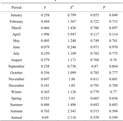
The results of testing the series stationary revealed that Iran’s monthly and annual precipitation series are stationary. According to the stationary condition of the series, and considering the rainfall intercept and slope changes, the simultaneous analysis of monthly and annually rainfall series variability was examined. In Table 2, the characteristics of the variability in the intercept and slope models have been found, and they were at significant levels. According to the weak changes of gradient, the non-stationary trend in the level of the series can be determined.

Table 2 Characteristics of the volatility in the intercept and slope models

Period F Χ2 _P

January 0.258 0.799 0.855 0.849 February 0.444 1.367 0.722 0.713 March 0.466 1.436 0.706 0.697

April 1.996 5.947 0.117 0.114 May 0.405 1.248 0.749 0.741 June 0.079 0.246 0.971 0.970 July 0.359 1.109 0.782 0.775 August 0.379 1.171 0.768 0.76 September 0.238 0.736 0.87 0.864

October 0.356 1.099 0.785 0.777 November 0.607 1.86 0.611 0.601 December 0.341 1.05 0.795 0.788 Winter 0.365 1.126 0.779 0.77 Spring 0.525 1.61 0.665 0.656 Summer 0.486 1.496 0.692 0.683 Autumn 0.765 2.341 0.515 0.504 Annual 0.69 2.116 0.559 0.549

However, using stationary testing, the stationary monthly and annual precipitation series was confirmed. Figure 2 showed the stationary condition of the monthly series and also the annual series.

Figure 2 The distribution of PACF and ACF 

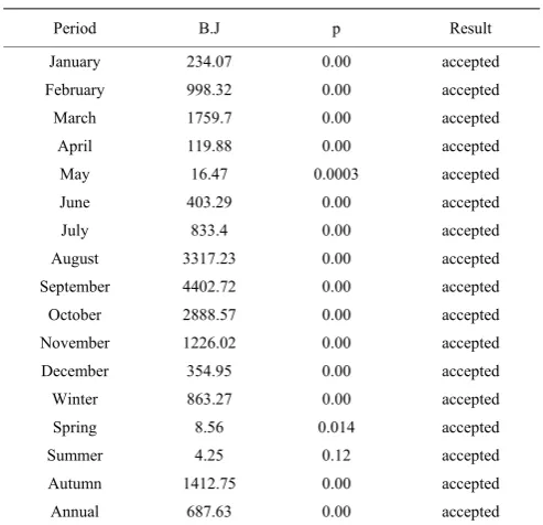
The results of distribution with accompanying t significant test are specified in Table 3.

Table 3 Results of B.J test

Period B.J p Result January 234.07 0.00 accepted February 998.32 0.00 accepted

March 1759.7 0.00 accepted April 119.88 0.00 accepted May 16.47 0.0003 accepted June 403.29 0.00 accepted

July 833.4 0.00 accepted

August 3317.23 0.00 accepted September 4402.72 0.00 accepted

October 2888.57 0.00 accepted November 1226.02 0.00 accepted December 354.95 0.00 accepted

Winter 863.27 0.00 accepted Spring 8.56 0.014 accepted Summer 4.25 0.12 accepted Autumn 1412.75 0.00 accepted

Annual 687.63 0.00 accepted

In addition, Figure 2 shows the normal distribution of the series. At the next stage of research using

Brock-Dechert-Scheinkman (BDS) and the logarithm of the initial series, the condition of rainfall non-linear series was studied and measured.

Table 4 shows the results of the BDS test in rainfall series. The results of test, confirmed the non-linear condition for stations annual precipitation, and the rainfall variability in Iran’s stations confirmed the condition of nonlinear models.

Finally, according to fluctuations or absence of oscillation (chaos) in the annual series, using overlapping variance ratio test, including the Pure Random Walk, Exponential Random Walk, and Innovation Random Walk, in order to review and testing of randomness of the series. Overlapping variance ratio test follows the Z distribution to interpret the results and hypothesis testing. Therefore, the test results showed that for 99% confidence level Iran’s annual rainfall series does not follow a random walk theory. The results of overlapping variance ratio test have been specified in Table 5.

Table 4 Results of BDS test for Iran rainfall

January February March Dimension BDS Statistic Std. Error z-Statistic Dimension BDS Statistic Std. Error z-Statistic Dimension BDS Statistic Std. Error z-Statistic

2 0.011884 0.008143 1.459419 2 0.003371 0.008325 0.404908 2 0.002063 0.007195 0.286763 3 0.014827 0.013027 1.138112 3 0.005744 0.013338 0.430655 3 0.005289 0.011482 0.460664 4 0.015344 0.015620 0.982354 4 0.005746 0.016016 0.358777 4 0.006796 0.013730 0.495011 5 0.011864 0.016394 0.723710 5 0.002866 0.016835 0.170233 5 0.006033 0.014370 0.419805 6 0.013311 0.015921 0.836043 6 0.001591 0.016375 0.097158 6 0.002174 0.013916 0.156226

April May June Dimension BDS Statistic Std. Error z-Statistic Dimension BDS Statistic Std. Error z-Statistic Dimension BDS Statistic Std. Error z-Statistic

2 0.010004 0.004967 2.014156 2 0.001875 0.005532 0.338885 2 –0.000755 0.012812 –0.058958 3 0.016837 0.007886 2.134944 3 0.004940 0.008821 0.559941 3 0.003771 0.020614 0.182919 4 0.016600 0.009379 1.769943 4 0.004724 0.010538 0.448293 4 0.003216 0.024879 0.129260 5 0.020188 0.009761 2.068211 5 0.010775 0.011017 0.977993 5 0.004998 0.026296 0.190073 6 0.020166 0.009399 2.145555 6 0.011907 0.010657 1.117360 6 0.000353 0.025728 0.013739

July August September

Dimension BDS Statistic Std. Error z-Statistic Dimension BDS Statistic Std. Error z-Statistic Dimension BDS Statistic Std. Error z-Statistic 2 –0.008700 0.012382 –0.702626 2 –0.006904 0.012261 –0.563079 2 –0.004401 0.013585 –0.323930 3 –0.009001 0.019919 –0.451884 3 –0.017486 0.019729 –0.886330 3 –0.016843 0.021896 –0.769250 4 –0.012294 0.024037 –0.511451 4 –0.016615 0.023810 –0.697841 4 –0.020422 0.026476 –0.771359 5 –0.006610 0.025401 –0.260237 5 –0.015402 0.025164 –0.612092 5 –0.016238 0.028039 –0.579131 6 –0.004711 0.024846 –0.189628 6 –0.013873 0.024616 –0.563559 6 –0.012723 0.027488 –0.462849

October November December Dimension BDS Statistic Std. Error z-Statistic Dimension BDS Statistic Std. Error z-Statistic Dimension BDS Statistic Std. Error z-Statistic

Table 5 Results of pure random walk, exponential random walk and innovation random walk tests

Pure Random Walk Exponential Random Walk

Innovation Random Walk Period

Var. Ratio z-Statistic Var. Ratio z-Statistic Var. Ratio z-Statistic 2 0.607125 –2.322501 0.628882 –3.737605 1.092069 0.834260 3 0.387300 –2.657345 0.381169 –4.286919 1.059104 0.382998 4 0.265468 –2.751746 0.272187 –4.086829 1.029047 0.159388 5 0.195827 –2.736105 0.208126 –3.832882 1.041345 0.201935 6 0.178749 –2.584959 0.180149 –3.535252 1.105693 0.461939 7 0.151633 –2.491034 0.151036 –3.331089 1.181016 0.712455 8 0.128360 –2.407808 0.115168 –3.210925 1.264847 0.951622 9 0.150798 –2.225090 0.145220 –2.903739 1.365611 1.215562 10 0.125652 –2.187439 0.121747 –2.815886 1.425962 1.326407 11 0.109086 –2.139816 0.104507 –2.726357 1.468916 1.380799 12 0.104602 –2.074466 0.100015 –2.615776 1.505431 1.418341 13 0.087142 –2.048571 0.076364 –2.575127 1.520417 1.400715 14 0.089888 –1.985391 0.085584 –2.455380 1.546666 1.418688 15 0.092369 –1.930529 0.090617 –2.359785 1.566990 1.424912 16 0.068997 –1.935721 0.074975 –2.326509 1.566065 1.382478

In the fourth stage of the research, for the predictability of the series based on a calculated variance comparison at various intervals, overlapping variance ratio test of Lo and McKinley was used. The results showed that predictability of monthly precipitation is verifiable. In addition, by using the autocorrelation function, partial autocorrelation function, and White heteroscedasticity test, randomness of models was found. The results of the mentioned tests were shown in Table 6.

Table 6 Results of Ljung-Box test

Model Q-Statistic (lag length = 16)

Q2_-Statistic

(lag length = 16)

ARCH 15.384 11.188

GARCH 15.017 10.988

GJR 15.126 10.998

EGARCH 16.146 11.962

TARCH 15.11 10.993

ARCH-M 14.221 8.469

MGARCH 14.910 11.311

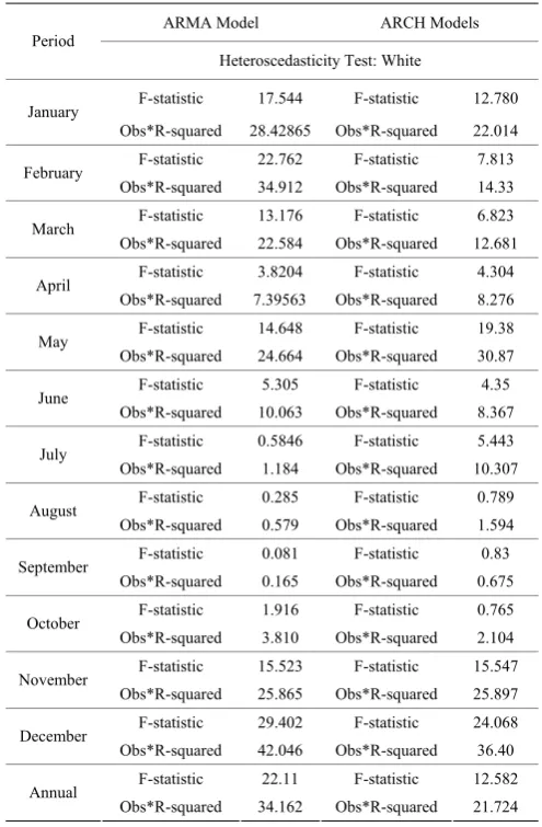
The results of the tests showed a random pattern, in both ARCH family models and ARIMA family models. Accordingly, the results of autocorrelation test were studied based on Ljung-Box test. Finally, by using the ARCH family models for the analysis of nonlinear time series and using the ARIMA family models to analyze the linear series, variability of Iran’s rainfall was predicted. Table 7 showed the efficiency of the used models.

The models findings based on indexes of the measuring accuracy were specified in Table 8.

Table 7 Results of heteroscedasticity test: white

ARMA Model ARCH Models Period

Heteroscedasticity Test: White

F-statistic 17.544 F-statistic 12.780 January

Obs*R-squared 28.42865 Obs*R-squared 22.014 F-statistic 22.762 F-statistic 7.813 February

Obs*R-squared 34.912 Obs*R-squared 14.33 F-statistic 13.176 F-statistic 6.823 March

Obs*R-squared 22.584 Obs*R-squared 12.681 F-statistic 3.8204 F-statistic 4.304 April

Obs*R-squared 7.39563 Obs*R-squared 8.276 F-statistic 14.648 F-statistic 19.38 May

Obs*R-squared 24.664 Obs*R-squared 30.87 F-statistic 5.305 F-statistic 4.35 June

Obs*R-squared 10.063 Obs*R-squared 8.367 F-statistic 0.5846 F-statistic 5.443 July

Obs*R-squared 1.184 Obs*R-squared 10.307 F-statistic 0.285 F-statistic 0.789 August

Obs*R-squared 0.579 Obs*R-squared 1.594 F-statistic 0.081 F-statistic 0.83 September

Obs*R-squared 0.165 Obs*R-squared 0.675 F-statistic 1.916 F-statistic 0.765 October

Obs*R-squared 3.810 Obs*R-squared 2.104 F-statistic 15.523 F-statistic 15.547 November

Obs*R-squared 25.865 Obs*R-squared 25.897 F-statistic 29.402 F-statistic 24.068 December

Obs*R-squared 42.046 Obs*R-squared 36.40 F-statistic 22.11 F-statistic 12.582 Annual

Obs*R-squared 34.162 Obs*R-squared 21.724 Note: Significance level: 1%.

Table 8 The criterions of ARMA model selection

Period Model CoefficientStandard_Error Indexes Model CoefficientStandard_Error

Annual AR(1) 0.9993 0.0016

AIC=14.137 SBIC=14.18 HQIC=14.154

MA(1) –0.9973 0.0132

Annual AR(1) 0.5871 0.0743 SBIC=14.571 AIC=14.529 HQIC=12.546

MA(2) 0.0361 0.0916

Annual AR(2) 0.9982 0.003

AIC=14.138 SBIC=14.181 HQIC=12.155

MA(2) –0.9931 0.0116

Annual AR(3) 0.99920 0.0046

AIC=14.159 SBIC=14.202 HQIC=14.177

MA(3) –0.9903 0.0158

Annual AR(4) 0.9928 0.0071

AIC=14.145 SBIC=14.188 HQIC=14.122

MA(4) –0.9733 0.0147

Annual AR(5) 0.9957 0.0077

AIC=14.171 SBIC=14.214 HQIC=14.188

MA(5) –0.9866 0.0163

Annual AR(6) 0.9859 0.0111 SBIC=14.205 AIC=14.161 HQIC=14.179

MA(6) –0.9637 0.0193

monthly precipitation was predicted.

Table 9 The accuracy indexes of models

Model RMSE MAE MAPE MSE Theil’s U ARIAM 279.33 168.68 78.68 78025.245 0.375 ARCH 426.85 322.82 100 182200.92 1 ARCH-M 279.43 173.156 83.704 78081.12 0.367 GARCH 279.83 170.73 80.81 78304.83 0.377

GIR 426.85 322.82 100 182200.92 1 TGARCH 426.85 322.82 100 182200.92 1 EGARCH 426.85 322.82 100 182200.92 1 Hybrid model 277.53 167.68 79.68 77025.34 0.365

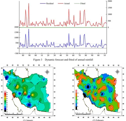
Figure 4 shows the condition of predicted values of rainfall series in Iran. According to the precision indicators of linear and non-linear models, it was observed that linear models are better for predicting the variability of Iran’s precipitation (Figure 3).

According to the Table 9, it is clear that the efficiency of Hybrid models is more suitable than the other models to predict the variability of monthly precipitation in Iran. According to this, by using the mentioned models, the

variability of monthly precipitation in Iran was predicted. According to Figure 4-1, by using the mentioned models the variability of January precipitation in the Iran was predicted. The results showed that the predictability of January precipitation is verifiable. The spread of spatial variability in the precipitation of the January is between 48 and 49 mm, including more than the half of Iran's areas and the highest variability can be seen in the southwestern of Iran (Khuzestan) and the lowest variability can be seen scattered in Iran. The results showed diversity in predictability of the February precipitation (Figure 4-2). The spread of spatial variability in the precipitation in February is between 90 and 100 mm, so that more than the half of Iran’s areas are surrounded and the highest variability can be seen at the center, east, and western north of Iran, and the lowest variability can be seen scattered in Iran. The results showed diversity in predictability of March precipitation (Figure 4-3).

Figure 3 Dynamic forecast and fitted of annual rainfall

(3) March (4) April

(5) May (6) June

(7) July (8) August

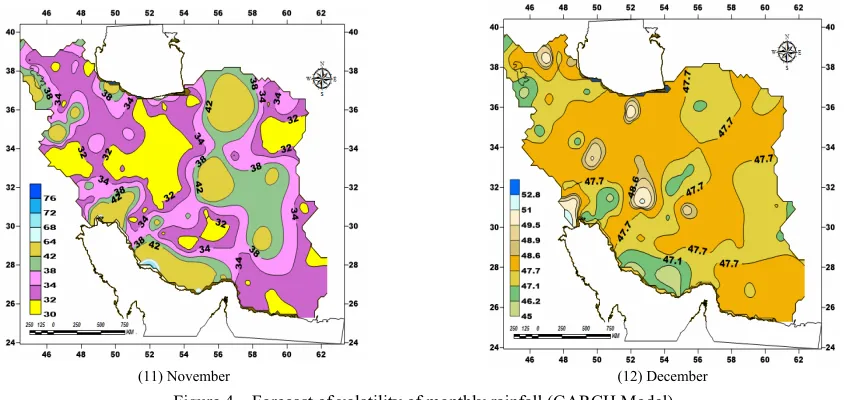
(11) November (12) December Figure 4 Forecast of volatility of monthly rainfall (GARCH Model)

The spread of spatial variability in precipitation of March is between 44 and 59 mm, so that almost all of the Iran’s areas are surrounded and highest variability can be seen in the northern half of Iran, and the lowest variability can be seen in the western south of Iran. The results showed diversity in predictability of April precipitation (Figure 4-4). The spread of spatial variability in precipitation of April is between 1 and 17 mm, so that almost half of the Iran’s areas are surrounded and the highest variability can be seen in the western north of Iran and the lowest variability can be seen in center and eastern south of Iran. The results showed variability predictability of May precipitation (Figure 4-5). The spread of spatial variability in precipitation of May is between 18 and 22 mm, so that almost the half of Iran’s areas are surrounded and the highest variability can be seen in the center and eastern north of Iran, and the lowest variability can be seen in eastern south of Iran. The results showed variability predictability of June precipitation (Figure 4-6). The spread of spatial variability in precipitation of June is between 6 and 6.5 mm, so that almost more than the half of Iran's areas are surrounded and the highest variability can be seen in the center and eastern south of Iran and the lowest variability can be seen in the center, east and eastern south of Iran. The results showed the variability predictability of July precipitation (Figure 4-7). The spread of spatial variability in precipitation of July is between 3 and 5 mm, so that almost the half of Iran's areas are surrounded and the highest variability can be seen in the center and western south of Iran and the lowest

variability in precipitation of December is between 47.7 and 48.1 mm, so that almost all the Iran's areas are surrounded, and the highest variability can be seen in center and eastern south of Iran and the lowest variability can be seen in western south of Iran. The results showed the diversity predictability of annual precipitation (Figure 5). The spread of spatial variability in precipitation in period using ARIMA model is between 93 and 639 mm, so that almost all the Iran’s areas are surrounded and the highest variability can be seen in eastern and south of Iran and the lowest variability can be scattered in west and north of Iran.

Figure 5 Forecast of variability of annual rainfall (ARIMA Model)

Figure 6 Forecast of variability of annual rainfall (GARCH (1, 1) Model)

Figure 7 show hybrid model during the predicted period for annual rainfall series, respectively.

The spread of spatial variability in precipitation in

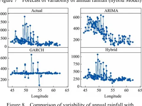
period using hybrid model is between 130 and 1027 mm, so that almost all the Iran’s areas are surrounded and the highest variability can be seen in central and eastern south of Iran and the lowest variability can be scattered in west and north of Iran. Figure 8 shows the rainfall predictions of the three models applied in this study using longitude for predicting annual rainfall.

Figure 7 Forecast of variability of annual rainfall (hybrid Model)

Figure 8 Comparison of variability of annual rainfall with longitude (models)

The spread of longitude variability in precipitation in period using three models are between 45 and 52 degrees, so that almost all the Iran’s areas are surrounded and the highest variability can be seen in east of Iran and the lowest variability can be scattered in west of Iran. Figure 9 show the rainfall predictions of the three models applied in this study using latitude for predicting annual rainfall.

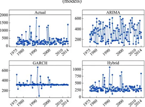
lowest variability can be scattered in north of Iran. Figure 10 show the rainfall predictions of the three models applied in this study using period for predicting annual rainfall.

Figure 9 Comparison of variability of annual rainfall with latitude (models)

Figure 10 Comparison of variability of annual rainfall with period (models)

The span of temporal variability in precipitation using three models are between 1990 and 2000 periods, so that almost all the Iran’s areas are surrounded and the highest variability can be seen in central parts of Iran and the lowest variability can be scattered in north of Iran.

4 Conclusions

In this study, the linear and nonlinear models in rainfall were determined for the 140 stations in a period of 40 years (1975-2014). This was carried out by using the ARCH family models, ARIMA models, and spatial variability analysis patterns. The variability patterns of rainfall were also estimated over the study period (1975-2014). Further, the spatial variability in monthly and annual rainfall was determined using the IDW interpolation method. The presentation of the

ARIMA-GARCH (1, 1) indexes can be added perfected, by using the validation and accuracy criteria. The variability in both upward and downward patterns was observed by the ARIMA-GARCH (1, 1) in monthly and annual rainfall in the 140 stations. All of the significant variability in monthly and annual rainfall was found at the 5% level of significance. However, significant variability in monthly rainfall was observed. Quantitative analysis shows that ARIMA-GARCH (1, 1) model (hybrid model) indicated the statistically significant obtains in the analytical model evaluated to other models, and that obtaining the dynamics of the linear and nonlinear models returns does develop the forecast of the rainfall conditional variability. Results indicated that there are various spatial-trend variation patterns that affect precipitation in Iran. The findings also indicated that among the rainfall data which were influential on precipitation, annual and then monthly precipitation had the highest spatial variations on the rate of precipitation. After all, the tem-poral-spatial patterns affects the precipitation rate in Iran and the spatial variability model, can show the magnitude of these variations on the precipitation changes rate and can examine the variation patterns well.

Acknowledgements:

This research was supported at PayameNoor University. We also thank PayameNoor management and research committee of PayameNoor University. Competing interests: The author declares that there are no competing interests regarding the publication of this article.

References

Abounoori, E., Z. Elmi, and Y. Nademi. 2016. Forecasting Tehran stock exchange volatility; Markov switching GARCH approach. Physica A: Statistical Mechanics and its Applications, 445: 264–282.

Babu, C. N. and B. E. Reddy. 2014. A moving-average filter based hybrid ARIMA–ANN model for forecasting time series data. Applied Soft Computing, 23: 27–38.

Badescu, A., R. J. Elliott, and J. P. Ortega. 2015. Non-Gaussian GARCH option pricing models and their diffusion limits. European Journal of Operational Research, 247(3): 820–830. Box, G. E. and D. A. Pierce. 1970. Distribution of residual

time series models. Journal of the American statistical Association, 65(332): 1509–1526.

Calzolari, G., R. Halbleib, and A. Parrini. 2014. Estimating GARCH-type models with symmetric stable innovations: Indirect inference versus maximum likelihood. Computational Statistics & Data Analysis, 76: 158–171.

Chambers, J. M., W. S. Cleveland, B. Kleiner, and P. A. Tukey. 1983. Graphical Methods for Data Analysis. Belmont, United States: Thomson Wadsworth.

Chan, J. C. C. and A. L. Grant. 2016. Modeling energy price dynamics: GARCH versus stochastic volatility. Energy Economics, 54: 182–189.

Chattopadhyay, S., D. Jhajharia, and G. Chattopadhyay. 2011. Trend estimation and univariate forecast of the sunspot numbers: Development and comparison of ARMA, ARIMA and autoregressive neural network models. Comptes Rendus Geoscience, 343(7): 433–442.

Chen, M. and K. Zhu. 2015. Sign-based portmanteau test for ARCH-type models with heavy-tailed innovations. Journal of Econometrics, 189(2): 313–320.

Cleveland, W. S. 1984. Graphs in scientific publications. The American Statistician, 38(4): 261–269.

Cleveland, W. S. and R. McGill. 1984. Graphical perception: Theory, experimentation, and application to the development of graphical methods. Journal of the American Statistical Association, 79(387): 531–554.

Costa. A. C, and A. Soares. 2009. Homogenization of climate data: review and new perspectives using geostatistics. Mathematical Geosciences, 41(3): 291–305.

Craves, F. B., B. Zalc, L. Leybin, N. Baumann, and H. H. Loh. 1980. Antibodies to cerebroside sulfate inhibit the effects of morphine and beta-endorphin. Science, 207(4426): 75–76. Efron, B. 1982. The Jackknife, the Bootstrap, and Other

Resampling Plans. Philadelphia, America: Siam.

Farajzadeh, J., A. F. Fakheri, and S. Lotfi. 2014. Modeling of monthly rainfall and runoff of Urmia lake basin using “feed-forward neural network” and “time series analysis” model. Water Resources and Industry, 7–8: 38–48.

Gouriéroux, C. 2012. ARCH models and financial applications. Berlin, Germany: Springer Science and Business Media. Hafner, C. M., and A. Preminger. 2015. An ARCH model without

intercept. Economics Letters, 129: 13–17.

Harvey, A., and G. Sucarrat. 2014. EGARCH models with fat tails, skewness and leverage. Computational Statistics and Data Analysis, 76: 320–338.

Javari, M. 2016. Spatial-temporal variability of seasonal precipitation in Iran. The Open Atmospheric Science Journal, 10(4): 84.

Javari, M. 2017a. Assessment of temperature and elevation controls on spatial variability of rainfall in Iran. Atmosphere, 8(3): 45. Javari, M. 2017b. Efficiency comparison of kernel interpolation

functions for investigating spatial variability of temperature in

Iran International Journal of Environmental and Science Education (IJESE), 12(4): 653–664

Javari, M.. 2017c. Spatial monitoring and variability of daily rainfall in Iran. International Journal of Applied Environmental Sciences, 12(5): 801.

Javari, M. 2017d. Spatial variability of rainfall trends in Iran. Arabian Journal of Geosciences, 10(4): 78.

Koul, H. L., and X. Zhu. 2015. Goodness-of-fit testing of error distribution in nonparametric ARCH(1) models. Journal of Multivariate Analysis, 137: 141–160.

Li, X., G. Zhai, S. Gao, and X. Shen. 2015. Decadal trends of global precipitation in the recent 30 years. Atmospheric Science Letters, 16(1): 22–26.

Liu, H., H. Tian, D. Pan, and Y. Li. 2013. Forecasting models for wind speed using wavelet, wavelet packet, time series and Artificial Neural Networks. Applied Energy, 107: 191–208. Ljung, G. M., and G. E. Box. 1978. On a measure of lack of fit in

time series models. Biometrika, 65(2): 297–303.

Mendes, R. R. A., A. P. Paiva, R. S. Peruchi, P. P. Balestrassi, R. C. Leme, and M. B. Silva. 2016. Multiobjective portfolio optimization of ARMA–GARCH time series based on experimental designs. Computers and Operations Research, 66: 434–444.

Mihailović, D. T., N. Drešković, and G. Mimić. 2015. Complexity analysis of spatial distribution of precipitation: an application to Bosnia and Herzegovina. Atmospheric Science Letters, 16(3): 324–330.

Narayan, P. K., R. Liu, and J. Westerlund. 2016. A GARCH model for testing market efficiency. Journal of International Financial Markets, Institutions and Money, 41: 121–138. Narayanan, P., A. Basistha, S. Sarkar, and S. Kamna. 2013. Trend

analysis and ARIMA modelling of pre-monsoon rainfall data for western India. Comptes Rendus Geoscience, 345(1): 22–27. Noureldin, D., N. Shephard, and K. Sheppard. 2014. Multivariate

rotated ARCH models. Journal of Econometrics, 179(1): 16–30. Santos, E. B., P. S. Lucio, and C. M. S. E. Silva. 2015.

Precipitation regionalization of the Brazilian Amazon. Atmospheric Science Letters, 16(3): 185–192.

Shi, X., and M. Kobayashi. 2009. Testing for jumps in the EGARCH process. Mathematics and Computers in Simulation, 79(9): 2797–2808.

Shimizu, K. 2014. Bootstrapping the nonparametric ARCH regression model. Statistics and Probability Letters, 87; 61–69. Souri, A. 2012. Econometrics: Noor Alm and Farhanshnasi. Iran. Tian, S., and S. Hamori. 2015. Modeling interest rate volatility: A

realized GARCH approach. Journal of Banking and Finance, 61: 158–171.

Xekalaki, E., and S. Degiannakis. 2010. ARCH models for financial applications. New York, America: John Wiley and Sons, Inc. Yan, Q., and C. Ma. 2016. Application of integrated ARIMA and