The Design of Robotic Arm Adaptive Fuzzy Controller Based on Oscillator and Differentiator

(1)

The Design of Robotic Arm Adaptive Fuzzy Controller

Based on Oscillator and Differentiator

https://doi.org/10.3991/ij ijoe.v15i05.8895

Min Wan, Qinglan Tian(*)_{,Chuanhong Sun, Xiuyuan Yi}

Southwest Petroleum University, Chengdu, China

Abstract—This paper mainly obtains the value of the state variable by de-signing the differentiator. The value of the state variable is necessary to track the manipulator with adaptive fuzzy controller. But difficult to obtain directly. In this paper, a model based on the dynamics analysis of robotic arm was build to design the second order oscillator and the Second Order differentiator in finite time to obtain the value of each state variable. The designed adaptive fuzzy controller for robotic arm achieved high accuracy in trace tracking. Simulation results of two-link robotic arm show the adaptive fuzzy controller for robotic arm based on differentiators is adaptable, flexible. This controller is simple to design, easy to implement, and has a good value for the application of robotic arm system. Keywords—Robotic arm, Adaptive Fuzzy Controller, Second Order Oscillator, Second Order differentiator in finite time

1

Introduction

(2)

value of state variables. In this thesis, the adaptive fuzzy controller realized high-precision tracking of robotic arm.

2

Dynamic Modeling and Analysis of Robotic Arm

According to Lagrange equation , where is the Lagrange function; is the total kinetic energy of the robotic arm; is the potential energy of it. Taking into account the friction and other disturbance vectors, we have the general dynamic equation of a double-joint robotic arm system, which reflects the functional relation among motion displacement, velocity, acceleration [11]:

(1)

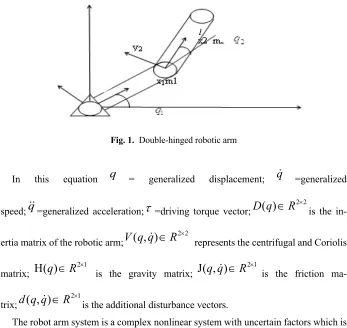
Fig. 1. Double-hinged robotic arm

In this equation = generalized displacement; =generalized

speed; =generalized acceleration; =driving torque vector; is the

in-ertia matrix of the robotic arm; represents the centrifugal and Coriolis

matrix; is the gravity matrix; is the friction

ma-trix; is the additional disturbance vectors.

The robot arm system is a complex nonlinear system with uncertain factors which is difficult to establish accurate mathematical models. Therefore, an adaptive fuzzy con-troller independent of precise mathematical model is designed in this paper.

L K P

= -

L

K

P

( )

( , )

H( ) J( , )

( , )

D q q V q q q

q

q q d q q

t

=

!!

+

! !

+

!

+

!

q

!

q

!!

t

D q

( )

Î

R

2 2´

2 2

( , )

V q q

!

Î

R

´

2 1

H( )

q

Î

R

´

J( , )

q q

!

Î

R

2 1´

2 1

( , )

d q q

!

Î

R

´

(3)

3

Design of Adaptive Fuzzy Controller

Consider MIMO Nonlinear Systems [12]:

(2)

where the state variables is measurable,

is input variables; is output

varia-bles; and are unknown smooth nonlinear functions . In this equation

Then formula (2) can be expressed as

(3)

By designing the control law , all variables are ensured to be bounded, and the

output of the system can track the desired trajectory . 1

( )

1 1 1

1

( )

1

( )

p

p r

j j

j

p r

p p pj j

j

y

f x

g x u

y

f x

g x u

=

+

=

+

å

!

1 ( 1)

( 1)

1 1 1

[ , , ,

r

, , ,

rp

]

T

p p

x

=

y y

! "

y

-

"

y y

-1

[ , , ]

T p

u u

=

!

u

y

=

[ , , ]

y

1

!

y

p T

( )

i

f x

g x

ij

( )

( ,

i j

=

1,2, , )

!

p

1 ( )

1

[

r

,

rp

]

r T

p

y

=

y

!

y

1

( )

[ ( ),

( )]

T p

F x

=

f x

!

f

x

11 1

1

( ) ( )

( )

( ) ( )

p

p pp

g x g x

G x

g x g x

é ù

ê ú

= ê ú

ê ú

ë û

!

" # "

!

( )r

( )

y

=

F x

+

G x u

( )

u t

1

( ) [ ( ), ,

( )]

T

d d dp

(4)

Hypothesis 1: It is a positive definite matrix, and there exist a real

num-ber , which satisfies ;

Hypothesis 2: Desired trajectory , is bounded, and there is

order derivative, and each order of the derivative are also bounded.

Hypothesis 1 can guarantee that the inverse of exists, then Formula (2) can be expressed as a linear form of the static state feedback, although assumptions are strictly limited to a MIMO system, the robotic arm system can satisfy the following assump-tions:

Define trajectory tracking error as

(4)

Define the error function of filter tracking as:

, (5)

,

As Formula (5) shows, when , , the control object

can be transformed into the . According to Newton's binomial theorem

(6)

( )

G x

0

s

>

G x

( )

³

s

₀

I

_p

( )

di

y t

i

=

1,2, ,

!

p

i

r

( )

G x

1( ) 1( ) 1( )

( ) ( ) ( )

d

p dp p

e t y t y t

e t y t y t

=

-=

-!

1 1 1

( )

(

d

1

)

r 1

( )

s t

e t

dt

l

-=

+

1

0

l

>

1

( ) ( )rp ( )

p d p p

s t e t

dt

l

-= +

l

_p

>

0

i

s

®

e

i

®

0( 1,2, , )

i

=

!

p

0( 1,2, , )

i

s

®

i

=

!

p

0

( )n n i i n i n i

a b C a b

-=

(5)

Where is binomial expansion coefficient. Apply Formula (6) to Formula (5) get

(7) then (8) which is (9) where (10) , , ! ( )! ! i n n C

n i i

= -1 1 1 1 1 0 1 1 ( 1)! ( ) ( ) ( ) ( ) ( )

( 1 )! !

( 1)! _{( )} _{( )}

( )!( 1)!

i i

i

r

r i j r j

i i i i i

j i r r j j i i i j i r d d

s t e t e t

dt r j j dt

r d _{e t}

r j j dt

l

-- -= -= -= + = -= -

-å

å

1 ( ) ( ) ( ) 1 1 1 ( ) ( ) ( ) 1 ( ) 1

( 1)! ( 1)!

( ) ( )

( )!( 1)! ( )!( 1)!

( 1)! _{( )} ( )!( 1)!

( 1)! ( ) ( )

( )!( 1)

i i

i i i

i

i i i

i

i i

r r

r j r r j

j j

i i

i i i i i i

j i j i

r

r r i j r j

d i i i

j i i

r i

d i ij j

j i

r r

s t e e e t

r j j r j j

r

y y e t

r j j

r

y f x g x u

r j j

l l l -- -= = -= = - -= = + - - - -= - + - -= - - + -

-å

å

! 1 ( ) 1 ( ) ! i i r r j j i i j

e t l

-=

å

1 1 1 1

1 1

( )

p j j j p

p p p pj j

j

s t

v

f x

g x u

s t

v

f x

g x u

= =

= -

-=

-

-å

å

!

"

!

1 1 1 1

( ) ( 1)

1 1, 1 1 1,1 1

( ) ( 1)

, 1 ,

p p

r r

d r

r r

p d p r p p p p

v

y

e

v

y

e

b

-=

+

=

+

!

"

!

,

(

i

)!(

1)!

r ji

i j i

i

r

r j j

b

=

-

l

(6)

Make , then

(11)

In a practical system, the nonlinear function and are unknown, fuzzy system can be used to approximate the non-linear function.

Assuming the fuzzy system is a mapping from to ,and

. The lth fuzzy rules can be expressed as

: IF is and and is , THEN is

where , are input and output of the fuzzy system.

Introduce Singleton fuzzifier, product inference engine and the center average de-fuzzifier into the design of fuzzy systems, the output of the fuzzy system

(12)

where is the corresponding value to the maximum of the membership ,which

is

then Formula (12) can be written as then Formula (12) can be written as

(13) 1

( ) [ ( ), , ( )]

T p

s t

=

s t

!

s t

v t

( ) [ ( ), , ( )]

=

v t

1

!

v t

p T

( )

s v F x G x u

!

= -

-( )

i

f x

g x

_ij

( )

n

U R

Í

R

1 n

,

i

( 1, , )

U U

=

´ ´

!

U U

Ì

R i

=

!

n

( )l

R

x

1

F

1l _!

x

n

F

nl

y

l

C

l

(

l

=

1,2, ,

!

M

)

1 2

[ , , , ]

T n

x

=

x x

!

x

Î

U

y V R

Î Ì

1 1

(

( ))

( )

(

( ))

i

M _l n

l

F i

l i

M n

l

F i

l i

y

x

y x

x

µ

= =

=

å Õ

l

y

l

c

µ

( ) 1

l

c

y

µ

=

( )

T

( )

(7)

where is the parameter vector, is the regression vector. Define

(14)

And the fuzzy system for approximating the nonlinear functions and is

, (15)

, (16)

where and is fuzzy basis function vectors; and is the adap-tive parameter vector.

Assume the best-fit parameters of and is and , the minimum fuzzy

approximation errors are and , which are defined as follows:

(17) (18) , (19) (20) (21) 1

[ , ,

y

M

]

q

=

!

x

( ) [ ( ), , ( )]

x

=

x

1

x

!

x

M

x

T

1 1 1

( )

(

( ))

i i n l F i i

l M n

l F i l i

x

µ

x

µ

= = =

=

Õ

å Õ

( )

i

f x

g x

_ij

( )

ˆ ( , )

_i T_i

( )

_i

i f f f

f x

q

=

x

q

i

=

1, ,

!

p

ˆ ( , )

_ij T_ij

( )

_ij

ij g g g

g x

q

=

x

q

i

=

1, ,

!

p

( )

i

f

x

_g_ij

( )

x

i

f

q

g_ij

i

f

q

g_ij

q

*f_i

* ij g

q

( )

i f

x

e

_g_ij

( )

x

*

arg min{sup | ( )

ˆ

( , ) |}

i i

fi x

f i i f

x D

f x

q

Î

=

-*

arg min{sup | ( )

ˆ

( , ) |}

ij ij

gij x

g ij ij g

x D

g x

q

Î

=

-*

i i i

f f f

q

!

=

q

-

q

*

ij ij ij

g g g

q

! =

q

-

q

*

ˆ

( )

( ,

)

i i

f

x

f x

i

f x

i f

e

=

-

q

*

ˆ

( )

( ,

)

ij ij

g

x

g

ij

x

g

ij

x

g

(8)

Assuming compact set is large enough, for all , the minimum

approxi-mation error is bounded, i.e. , ,among

them , . It is a known constant. Set

then

(22)

(23)

x

D

x D

Î

_x

| ( ) |

e

f_i

x

£

e

fi

( )

x

| ( ) |

e

gij

x

£

e

gij

( )

x

i

f

e

_g_ij

( )

x

1

ˆ

ˆ ( )

[

( ),

,

( )]

T

p

F x

=

f

x

!

f

x

11 1

1

ˆ ( ) ˆ ( )

ˆ ( )

ˆ ( ) ˆ ( )

p

p pp

g x g x

G x

g x g x

é ù

ê ú

= ê ú

ê ú

ë û

!

" # "

!

1

( )

[

( ),

,

_p

( )]

T

f

x

f

x

f

x

e

=

e

!

e

11 1 1 ( ) ( ) ( ) ( ) ( ) p p pp g g g g g x x x x x

e

é ù ê ú

= ê ú

ê ú

ë û

!

" # "

!

1

( ) [

( ),

,

_p

( )]

T

f

x

f

x

f

x

e

=

e

!

e

11 1 1 ( ) ( ) ( ) ( ) ( ) p p pp g g g g g x x x x x e e e e e é ù ê ú

= ê ú

ê ú

ë û

!

" # "

!

*

ˆ

( )

( , )

f

( , )

f

( , )

f f

( )

F x

-

F x

q

=

F x

q

-

F x

q

+

e

x

*

ˆ

( )

( , )

g

( , )

g

( , )

g g

( )

(9)

Use and to replace and , the control law is

(24)

Because is given by online estimating the value of , it is difficult to

ensure that is non-singularity. Thus, introducing the generalized inverse

to replace , then control law is

(25) where is a positive real number arbitrarily small, is the unit matrix.

In order to reduce the modeling errors, the robust controls was introduced, the control law is

(26)

(27)

(28) where It is a time-varying parameter.

Adaptive control law is

(29)

(30)

ˆ( , )

f

F x

q

G x

ˆ( , )

q

_g

F x

( )

G x

( )

1

0

ˆ

( , )(

ˆ

( , )

)

c g f

u

=

G x

-

q

-

F x

q

+ +

v K s

ˆ( , )

g

G x

q

_g

ˆ( , )

_g

G x

q

1 0

ˆ

T

( , )[

ˆ

( , ) ( , )]

ˆ

T

g p g g

G x

q e

I

+

G x

q

G x

q

-

ˆ ( , )

1

g

G x

-

q

0 2

0

| | (

| | | |)

|| ||

T

f g c

r

s s

u

s

e

s

d

+

=

+

0

e Ip

r u

c r

u u u

=

+

0 2

0

| | (

| | | |)

|| ||

T

f g c

r

s s

u

s

e

s

d

+

=

+

1

0 0

[

0 p

ˆ

( , ) ( , )] (

g

ˆ

T g

ˆ

( , )

f 0

)

u

=

e e

I

+

G x

q

G x

q

-

F x

q

+ +

v K s

d

( )

i i i

f f f

x s

i

q

!

= -

h x

( )

ij ij ij

g g g

x s u

i cj

(10)

(31)

where , , , .

While design the fuzzy controller, we assume that the state

varia-bles is measurable. For some immeasurable state, the following differentiator is adopted.

4

Design of Differentiator

4.1 Second-order Oscillation Link

and are the Laplace transform of input and output , the func-tion of the second-order oscillafunc-tion link is

(32)

set , ,then by the formula (32) available:

(33)

The Laplace transformation of Formula (33) is

(34)

so

0

0 2

0

| | (

| | | |)

|| ||

T

f g c

s

u

s

e

d

h

s

d

+

=

-+

!

0

i

f

h

>

h

g_ij

>

0

h

₀

>

0

d

(0) 0

>

1 ( 1)

( 1)

1 1 1

[ , , ,

r

, , ,

rp

]

T

p p

x

=

y y

! "

y

-

y y

-"

( )

V s X s( )

v t

( )

x t

( )

2

2 2

( )

2

n_n _n

X s

V s

s

w

xw

w

=

+

1( ) ( )

x t =x t x t2( )=x t!( )

1 2

2 2

2 n 1 n

( ) 2

n 2

x

w

x

w

v t

xw

x

=

ì

í

= -

+

-î

!

1 2

2 2

2 1 2

( )

_n

( )

_n

( ) 2

_n

( )

sX s

X s

sX s

w

X s

w

V s

xw

X s

=

ì

í

= -

+

(11)

(35)

Available

(36)

Therefore, when large enough, the system can eliminate the high frequency

noise, and the system output , i.e. derivative of the tracking signal .

4.2 Second Order differentiator in finite time

If using the second-order oscillation link to obtain the derivative of signal, theoret-ically it only convergence when time goes to infinity, so the Second Order differenti-ator in finite time was adopted. The Second Order differentidifferenti-ator in finite time can quickly converge in finite time, and there is no chattering occurs. In addition to the derivative of the signal that is derivable, the differentiator can also obtain some non-smooth generalized derivatives.

Hereby introducing four assumptions:

Hypothesis 1: Assuming the equilibrium of the following system is a stable in finite

time

(37) 2

2 2

( )

1

2

( )

(

1)

n n

X s

s

V s

s

z

s

w

=

+

2

( )

lim

( )

n

X s

s

V s

w®¥

=

n

w

2

( )

x t

v t

!

( )

v t

( )

1 2

1

1 2

( , , , )

n n

z

f z z

z

-ì =

ï

í

=

ï

ï =

î

!" "

#

!"

"

(12)

And the stop time function is continuous at the zero point, where is

con-tinuous and .N is the open neighborhood of the zero point. Then for the system formula (40), there is a continuous function that met: 1) is positive

defi-nite; 2) It is a real value, and is continuous in N; 3) there exists that satisfies

(38)

Hypothesis 2: There is a Lipschitz Function that satisfies Lyapunov Function,

function V satisfies the Formula (38) and the Lipschitz Constant of Lyapunov Function is M.

Hypothesis 3: For a system formula (37), there

are , and a non-negative constant satisfy

(39)

Hypothesis 4: Suppose is a segment signal that is continuously differentiable,

and satisfies the following properties: throughout the whole time domain, order

derivative of signal exists, and at some point , the order is

non-conductive. The order left derivative and right derivative

of signal both exist, and , . Based on the above assumptions, the second-order differentiator that converges in finite time is designed as follows:

f

T

f

()

(0) 0

f

=

V

!

c

>

₀

0

V cV

!

+

£

(0,1]

i

r

Î

i

=

0,1, ,

!

n

-

1

a

1

1 2, 1 2

1

| ( ,

, )

( , , , ) |

|

i

n

n n i i

i

f z z

z

f z z

z

a

z z

r

-=

-

£

å

-! -!

"

!

"

!

( )

v t

2

n

-( )

v t

t j

j

(

=

1, , )

!

k

n

-

1

n

-

v

-( 1)n-

( )

t

j

( 1)n

( )

j

v

-

t

(13)

(40)

(41)

where

(42)

There exist (where, and = =

), for

, ,where ,

, , thus we have

(43)

and established, where is the perturba-tion parameter, represents that the approximation error be-tween and is order, when . In fact, the system

(44) 1 2 2 2 2

x

u

y x

e

=

ì

ï

=

í

ï =

î

!

2

1 2 1 2 2 2

{sgn( ( ( ), )) | ( ( ), ) | } {sgn( ) | | }

b a a b

u sat x v t x x v t x aa sat x x a

e j e j e - e e

= - - -

-2

1 2 1

1

2 2

(

( ),

) |

( )

sgn( ) |

|

2

a

x v t x

x v t

x

a

j

e

a

--

= -

+

-| -|

( )

sgn( )

| |

b b b b

x

sat x

x

e

<

ì

= í

³

î

0

g

>

rl

>

2

r

min{ , / (2

a a

-

a

)}

/ (2

)

a

-

a

( ( ) (0))

t³ G Xe e e

i

=

1

X

( )

e

=

diag

{1, , ,

e

!

e

n-1

}

1

( ( ) ( ))

1

j j j

t

> ³

t t

_-

+ G X

e

e t

_-

j

=

1, ,

!

k

+

1,

i

=

2

( 1)i

( )

(

i 1

)

i

x v

-

t

=

O

e

rl-+

1

2

( )

j

( )

(

),

1, ,

x t

v t

e

rl-

j

k

-

¢

-

=

O

=

!

e

1

(

e

rl-i+

)

O

i

x

v t

i-1

( )

e

rl-i+1

a Î

(0,1)

1 2

2

2 b

{sgn( ( , )) | ( , ) | }

a 1 2 a 1 2 b

{sgn( ) | | }

2 2

x

sat

x x

aa

sat

x

a

e

j

- e

(14)

Converges at original point in a limited time , and satisfies assumptions .

For Formula (47), when , we

have established, which

(45)

The smaller is, the shorter the convergence time will be, the tracking smaller error will be. However, is too small, so that the derivative of the differentiator has a large peak near the initial time. worth selecting is detailed in the text. [13]

For this type of differentiator, in addition to obtaining the derivatives of the general continuous derivative signals, since the convergence time and the tracking error is sufficiently small, by selecting the derivative of some piecewise contin-uous signal can also be obtained.

5

Simulation Analysis

The Second Order differentiator in finite time is designed as follows：

(46)

Among them, ； is the tracking of the signal, an estimate of the

first derivative of the signal; Input signal ；The initial value of the

f

T

1 ~ 4

1 2

( 1,2,

i

1

,

2

[0, ))

t t

<

=

"

t t

Î

¥

2 1

| ( ) |

x

i

t

£

x

i

( )

t

2

1 2 1

1

2 2

( , )

sgn( ) | |

2

x x

x

a

j

a

-= +

-e

e

*

(0, )

e

Î

e

1 2

2 5/3 1/5 1/3

2 {( 1 ( ) 3₅( 2) ) } {( 2) }

, | | 1 ( ) _{sgn( ), | | 1}

x x

x sat x v t x sat x x x

sat x

x x

e e e

ì ï = ï ï

= - - +

-í ï

ï ₌ì <

ï í _³

î î

! !

=0.004

e

x

1

x

2

( ) 10sin

(15)

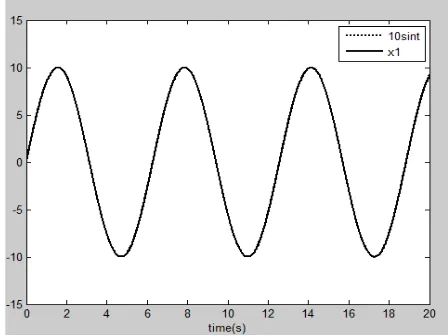
differentiator are , . The simulation results are shown in the figure 2.

Fig. 2. Finite time convergence differentiator signal tracking

Fig. 3. Finite-time convergence differentiator derivative estimation

The differentiator realizes filtering and derivation of the signal, and has a fast con-vergence speed. For rigid double-joint robotic arm in planar motion, if ignoring gravity, the dynamic equation is

1

(0) 0

(16)

(47)

It can be converted to

(48)

where

(49)

(50)

(51)

(52)

(53)

(54)

, (55)

Let

.

Among them is the quality of the first section of the arm, is the quality of

the second section of the arm is the length of the first section of the arm, is the

1

11 12 1 2 1 2 1 1

21 22 2 1 2 2 2

(

)

+

0

N

M

q

hq

h q q

q

u

M

q

hq

q

N

u

-

+

é

ù

é

ù é ù é

+

ù é ù

=

é ù

ê

ú

ê

ú ê ú ê

ú ê ú

ê ú

ë

û ë û ë

û ë û

ë

û

ë û

!!

!

!!

!

1

1 11 12 1 2 1 2 1

2 21 22 2 2 1 2

(

)

0

N

q

M

u

hq

h q q

q

M

u

N

hq

q

-ì

é

ù

-

+

ü

é ù é

=

ù

ï

é ù

-

é

ù é ù

ï

í

ê

ú

ý

ê ú ê

ú

ï

ê ú

ê

ú ê ú

ï

ë û ë

û

î

ë û

ë

û

ë

û ë û

þ

!!

!

!!

!

11 1

2 cos

3 2

2 sin ,

4 2 22 2

M

= +

a

q

+

a

q M

=

a

21 12 2 3

cos

2 4

sin

2

M

=

M

=

a a

+

q a

+

q

1

(

1 e

) cos

1 2 e c1

cos(

1 2

)

N

=

m m l

+

q m l

+

q q

+

2 e c1

cos(

1 2

)

N

=

m l

q q

+

3

sin

2 4

cos

2

h a

=

q a

-

q

2 2 2

1 1 1 1c e e ce e1

a = +I m l + +I m l +m l 2 2 e e ce

a

= +

I m l

3 e1cecos e

a =m l l d a₄ =m l l_e₁_cesind_e

1

1,

e

2,

1

1,

c1

0.5,

ce

0.6,

1

0.12,

e

0.25,

e

6

m

=

m

=

l

=

l

=

l

=

I

=

I

=

d

=

p

1

m me

(17)

length of the second section of the arm. is distance from the center of mass to the second joint, is the moment of inertia of the first arm, is the moment of inertia of the second arm, is the angle between the center of mass and the second arm.

, ,

The goal of controlling is to make the output of the system , track the desired

trajectory , . Define membership function as

,

Let

, , , , , , ,

, , .

The oscillation link can be written in its state-space form as

(56)

Let , , be the position signal for the robotic arm, is the estimation of the first derivative of it.

The Second Order differentiator in finite time is designed as follows,

ce

l

1

I Ie

e d

[

1 2

]

T

y

=

q q

u

=

[

u u

₁ ₂

]

T

x

=

[

q q q q

1

!

1 2

!

2

]

1

q

₂

1

sin

d

y

=

t

y

d₂

=

sin

t

1 2

1

1.25

( ) exp(

(

) )

2

0.6

i

i i

F

x

µ

=

-

+

2 2

1

( ) exp(

(

) )

2 0.6

i

i i

F

x

µ

=

-3 2

1

1.25

( ) exp(

(

) )

2

0.6

i

i i

F

x

µ

=

-

-1,2,3,4

i

=

1

30

l

=

l

₂

=

30

K

₀

=

5

I

₂

e

₀

=

0.1

0.5

i

f

h

=

h

_g_ij

=

0.5

h

0

=

0.001

(0) 0

d

=

0.2 0.2

g

e

=

é

ê

ù

ú

ë

û

[

0.2 0.2

]

T f

e =

1 2 2

2 n

(

1

( )) 2

n 2

x

w

x v t

zw

x

=

ì

í

=

-

-î

!

1000

n

(18)

Let be the position signal for the robotic arm, is the estimation of the first derivative of it.

Fig. 4. Tracking curves of position and velocity with the oscillation for link 1

Fig. 5. Tracking curves of position and velocity with the oscillation for link 2

0.0001

(19)

Fig. 6. Error of input signal and tracking signal based on oscillator

(20)

Fig. 8. Tracking curves of position and velocity with the differential for link 2

Fig. 9. Error of input signal and tracking signal based on differentiator

(21)

fluctuations in the early stage of position and speed tracking for link 1 and link 2, in the later period it can track the given trajectory smoothly.

6

Conclusion

Because fuzzy control system does not have to depend on accurate mathematical model, it is suitable for solving the control problem of the robotic arm. The fuzzy control system requires the value of the system state variables, though certain system state variables cannot or hardly be measured directly, hence introducing the sec-ond-order oscillator and the Second Order differentiator in finite time to obtain state variables.

In this paper, by using the designed adaptive fuzzy controller, the trajectory tracking control for robotic arm with high accuracy was realized. The simulation results show that the designed adaptive fuzzy controller for tracking robotic arm possessed high flexibility and adaptability. It is easy to realize, simple in structure, and also has a good value for the robotic application.

7

Acknowledgement

This project is supported by National Natural Science Foundation of China (grant no 51775463).

8

References

[1]Wang Tianmiao, Tao Yong. Research status and industrialization development strategy of Chinese industrial robot[J]. Journal of Mechanical Engineering, 2014,50(9):1-13.

https://doi.org/10.3901/JME.2014.09.001

[2]Ren Guohua. Mobile robot trajectory tracking and motion control [J]. Machinery Design and Manifacture, 2014, (3):100-102.

[3]Xu Z H, Lu T S. Adaptive fuzzy control for trajectory tracking of hopping robot[J]. Journal of System Simulation, 2008, 20(23):6455-6457.

[4]Khalate A A, Leena G, Ray G. An Adaptive Fuzzy Controller for Trajectory Tracking of Robot Manipulator [J]. Intelligent Control & Automation, 2015, 02(4):364-370.

https://doi.org/10.4236/ica.2011.24041

[5]Liu Guorong, et al. Direct adaptive fuzzy robust control for a class of nonlinear MIMO system[J]. Control Theory and Application,2003,20(5):697-698.

[6]Wu T S, Karkoub M, Chen H S, et al. Robust tracking observer-based adaptive fuzzy con-trol design for uncertain nonlinear MIMO systems with time delayed states[J]. Information Sciences, 2015, 290:86-105. https://doi.org/10.1016/j.ins.2014.08.001

(22)

[7]Li Y X, Yang G H. Observer-Based Fuzzy Adaptive Event-Triggered Control Co-Design for a Class of Uncertain Nonlinear Systems [J]. IEEE Transactions on Fuzzy Systems, 2017, PP (99):1-1.

[8]Gao Y, Tong S, Li Y. Observer-based adaptive fuzzy output constrained control for MIMO nonlinear systems with unknown control directions [M]. Elsevier North-Holland, Inc. 2016. [9]Li Y, Tong S, Li T. Observer-Based Adaptive Fuzzy Tracking Control of MIMO Stochastic Nonlinear Systems with Unknown Control Directions and Unknown Dead Zones[J]. IEEE Transactions on Fuzzy Systems, 2015, 23(4):1228-1241.

https://doi.org/10.1109/TFUZZ.2014.2348017

[10]Wan Min, An Lingzhi. Control system simulation research for double joints manipulator based on MATLAB [J]. Journal of Plasticity Engineering, 2017,24(6):136-142.

[11]Liu Jinkun. Robot control system and MATLAB simulation[M]. Beijing: Tsinghua Uni-versity Press,2013.

[12]Wang Xinhua, Liujinkun. Differentiator design and application-signal filtering and dif-ferentiation[M]. Publishing House of Electronics Industry,2010.

9

Authors

Min Wan received the B.S. degree in Automation from Dalian Maritime

Uni-versity, Dalian, China, in 2000 and the M.S. degree in Detection Technology and Automation Device from University of Electronic Science and Technology, Chengdu, China, in 2006. She is currently working toward the Ph.D. degree with the Institute of Mechanical and Electrical Engineering, Southwest Petroleum Uni-versity, Chengdu, China. Her current research interests include fuzzy logic system, stochastic adaptive control, and robot control.

Qinglan Tian received the B.S. degree in Automation from Shanghai University

Of Engineering Science, Shanghai, China, in 2016. She is currently working toward the M.S. degree with the Instrumentation Engineering, Southwest Petroleum Uni-versity, Sichuan, China. Her current research interest includes fuzzy control and adaptive control.

Chuanhong Sun is currently working toward the B.S. degree with the Process

Equipment and Control Engineering, Southwest Petroleum University, Sichuan, China. He current research interest includes process control and robot control.

Xiuyuan Yi is currently working toward the B.S. degree with the Process

Equipment and Control Engineering, Southwest Petroleum University, Sichuan, China. He current research interest includes process control and robot control.