BasicFeedbackStructures

(1)

C H A P T E R 4

Basic Feedback

Structures

T

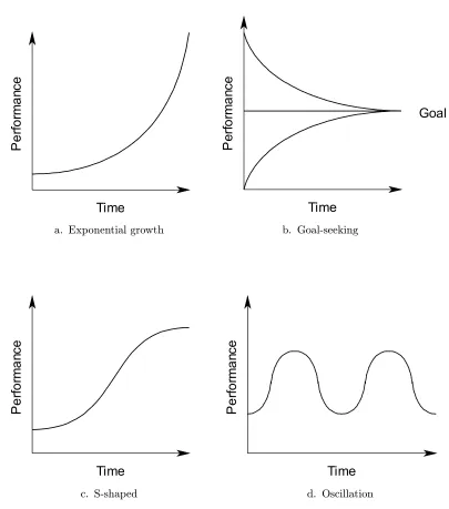
his chapter reviews some common patterns of behavior for business processes, and presents process structures which can generate these patterns of behavior. Many interesting patterns of behavior are caused, at least in part, by feedback, which is the phenomenon where changes in the value of a variable indirectly in®uence future values of that same variable. Causal loop diagrams (Richardson and Pugh 1981, Senge 1990) are a way of graphically representing feedback struc-tures in a business process with which some readers may be familiar. However, causal loop diagrams only suggest the possible modes of behavior for a process. By developing a stock and®ow diagram and corresponding model equations, it is possible to estimate the actual behavior for the process.

Figure 4.1 illustrates four patterns of behavior for process variables. These are often seen individually or in combination in a process, and therefore it is useful to understand the types of process structures that typically lead to each pattern.

4.1 Exponential Growth

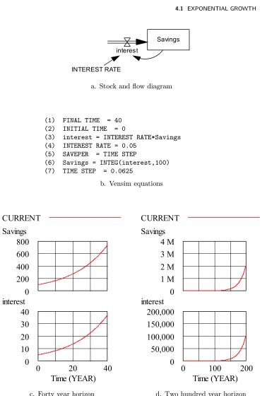
Exponential growth, as illustrated in Figure 4.1a, is a common pattern of be-havior where some quantity \feeds on itself" to generate ever increasing growth. Figure 4.2 shows a typical example of this|the growth of savings with com-pounding interest. In this case, increasing interest earnings lead to an increase in Savings, which in turn leads to greater interest because interest earnings are proportional to the level of Savings, as shown in equation 3 of Figure 4.2b. Fig-ure 4.2c shows the characteristic upward-curving graph that is associated with this process structure. This is referred to as an \exponential" curve because it can be demonstrated that it follows the equation of the exponential function. (Remember that the \cloud" at the left side of Figure 4.2a means that we are not explicitly modeling the source of the interest.)

(2)

Time

P

e

rf

o

rm

a

nc

e

a. Exponential growth

Time

P

er

fo

rm

a

nc

e

Goal

b. Goal-seeking

Time

P

e

rf

o

rm

a

nc

e

c. S-shaped

P

e

rf

o

rm

a

nc

e

Time

d. Oscillation

(3)

4.1 EXPONENTIAL GROWTH 31

INTEREST RATE interest

Savings

a. Stock and®ow diagram

(1) FINAL TIME = 40

(2) INITIAL TIME = 0

(3) interest = INTEREST RATE*Savings

(4) INTEREST RATE = 0.05

(5) SAVEPER = TIME STEP

(6) Savings = INTEG(interest,100)

(7) TIME STEP = 0.0625

b. Vensim equations

CURRENT

Savings

800

600

400

200

0

interest

40

30

20

10

0

20

40

Time (YEAR)

c. Forty year horizon

CURRENT

Savings

4 M

3 M

2 M

1 M

0

interest

200,000

150,000

100,000

50,000

0

100

200

Time (YEAR)

d. Two hundred year horizon

(4)

component of a more complex process in realistic settings. The models of those more complex processes usually cannot be solved in closed form, and therefore we have shown the Vensim simulation equations used to simulate this model in Figure 4.2b.

Figure 4.2d shows another characteristic of exponential growth processes. In this diagram, the time period considered has been extended to 200 years. When this is done, we see that exponential growth over an extended period of time displays a phenomenon where there appears to be almost no growth for a period, and then the growth explodes. This happens because with exponential growth the period which it takes to double the value of the growing variable (called the \doubling time") is a constant regardless of the current level of the variable. Thus, it will take just as long for the variable to double from 1 to 2 as it does to double from 1,000 to 2,000, or from 1,000,000 to 2,000,000. Hence, while the variables in Figure 4.2d are growing at a steady exponential rate during the entire 200 year period, because of the large vertical scale necessary for the graph in order to show the values at the end of the period, it is not possible to see the growth during the early part of the period.

4.2 Goal Seeking

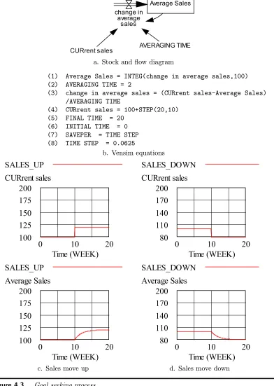
Figure 4.1b displays goal seeking behavior in which a process variable is driven to a particular value. Figure 4.3 presents a process which displays this behavior. As \CURrent sales" change, the level of Average Sales moves to become the same as CURrent sales. However, it moves smoothly from its old value to the CURrent sales value, and this is the origin of the name Average Sales for this variable. (In fact, this structure can be used to implement the SMOOTH function which we have previously seen.)

Figure 4.3c and Figure 4.3d show what happens when CURrent sales takes a step up (in Figure 4.3c) or a step down (in Figure 4.3d). While it is somewhat hard to see in these graphs, CURrent sales is plotted with a solid line which jumps at time 10. Until that time, Average Sales have been the same as CURrent sales, then they diverge since it takes a while for Average Sales to smoothly move to again become the same as CURrent sales.

Equation 3 in Figure 4.3b shows the process which drives Average Sales toward the value of CURrent sales. If Average Sales are below CURrent sales, then there is ®ow into the Average Sales stock, while if Average Sales are above CURrent sales, then there is ®ow out of the Average Sales stock. In either case, the®ow continues as long as Average Sales di¯ers from CURrent sales.

The rate at which the ®ow occurs depends on the constant AVERAGING TIME. The larger the value of this constant, the slower the ®ow into or out of Average Sales, and hence the longer it takes to bring the value of Average Sales to that of CURrent sales.

(5)

4.2 GOAL SEEKING 33

AVERAGING TIME CURrent sales

change in average

sales

Average Sales

(1) Average Sales = INTEG(change in average sales,100)

(2) AVERAGING TIME = 2

(3) change in average sales = (CURrent sales-Average Sales)

/AVERAGING TIME

(4) CURrent sales = 100+STEP(20,10)

(5) FINAL TIME = 20

(8) TIME STEP = 0.0625

b. Vensim equations

SALES_UP

CURrent sales

200

175

150

125

100

0

10

20

Time (WEEK)

SALES_DOWN

CURrent sales

200

170

140

110

80

0

10

20

Time (WEEK)

SALES_UP

Average Sales

200

175

150

125

100

0

10

20

Time (WEEK)

SALES_DOWN

Average Sales

200

170

140

110

80

0

10

20

Time (WEEK)

c. Sales move up d. Sales move down

(6)

possible to obtain a simple solution, and thus we show the simulation equations for this process.

Note that the process shown in Figure 4.4 is a negative feedback process. As the value of \change in average sales" increases, this causes an increase in the value of Average Sales, which in turn leads to a decrease in the value of \change in average sales."

4.3 S-shaped Growth

Exponential growth can be exhilarating if it is occurring for something that you makes you money. The future prospects can seem endlessly bright, with things just getting better and better at an ever increasing rate. However, there are usually limits to this growth lurking somewhere in the background, and when these take e¯ect the exponential growth turns into goal seeking behavior, as shown in Figure 4.1c.

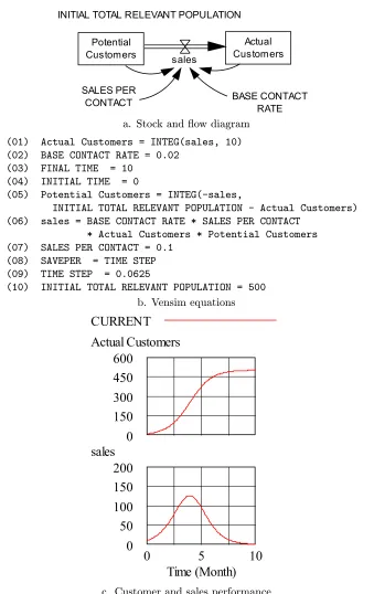
Figure 4.4 shows a business process structure which can lead to this \s-shaped" growth pattern. This illustrates a possible structure for the sale of some sort of durable good for which word of mouth from current users is the source of new sales. This might be called a \contagion" model of sales|being a user of the product is contagious to other people! We assume that there is a speci±ed INITIAL TOTAL RELEVANT POPULATION of potential customers for the product. (This is the limit that will ultimately stop growth in Actual Customers.) At any point in time, there is a total of \Potential Customers" of potential users who have not yet bought the product.

Visualize the process of someone in the Potential Customers group being con-verted into an Actual Customer as follows: The two groups of people who are in the Actual Customers group and in the Potential Customers group circulate among the larger general population and from time to time they make contact. When they make contact, there is some chance that the comments of the per-son who is an Actual Customer will cause the perper-son who is in the Potential Customers to buy the product.

(7)

4.3 S-SHAPED GROWTH 35

of contacts per unit time between any speci±ed member of the Actual Customers group and any speci±ed member of the Potential Customers group.)

The argument in the last paragraph for a multiplicative form for the \sales" equation (as shown in equation 6 of Figure 4.4b) was somewhat informal. A more formal argument can be made by using probability theory. Select a short enough period of time so that at most one contact can occur between any persons in the Actual Customers group and the Potential Customers group regardless of how large these groups are. Then assume that the probability that any speci±ed member of the Actual Customers group will contact any speci±ed member of the Potential Customers group during this period is some (unspeci±ed) number p. Then, if this probability is small enough (which we can make it by reducing the length of the time period considered), the probability that the speci±ed mem-ber of the Actual Customers group will contactany member of the susceptible population is equal top Potential Customers.

Assuming that this probability is small enough for any individual member of the Actual Customers population, then the probability thatany member of the Actual Customers population will contact a member of the Potential Customers population is just this probability times the number of members in the Actual Customers population, or

p susceptible population Actual Customers:

Assuming the interaction process between the two groups is a Poisson process and the probability of a \successful" interaction (that is, a sale) is±xed, then the sale process is a random erasure process on a Poisson process and hence is also a Poisson process. Thus, the expected number of sales per unit time is proportional to the probability expression above, and hence to the product of Actual Customers and susceptible population. This is the form assumed in equation 6 of Figure 4.4b.

Figure 4.4c shows the resulting pattern for the number of Actual Customer, as well as the sales. This s-shaped pattern is seen with many new products. First the process grows exponentially, and then it levels o¯. Sales also grow exponentially for a while, and then they decline. This can be a di cult process to manage because the limit to growth is often not obvious while the exponential growth is under way. For example, when a new consumer product like the compact disk player is introduced, what is the INITIAL TOTAL RELEVANT POPULATION of possible customers for the product? The di¯erence between a smash hit like the compact disk player and a dud like quadraphonic high±delity sound systems can be hard to predict.

(8)

BASE CONTACT RATE SALES PER

CONTACT

INITIAL TOTAL RELEVANT POPULATION

sales

Actual Customers Potential

Customers

(01) Actual Customers = INTEG(sales, 10)

(02) BASE CONTACT RATE = 0.02

(03) FINAL TIME = 10

(05) Potential Customers = INTEG(-sales,

INITIAL TOTAL RELEVANT POPULATION - Actual Customers)

(06) sales = BASE CONTACT RATE * SALES PER CONTACT

* Actual Customers * Potential Customers

(07) SALES PER CONTACT = 0.1

(09) TIME STEP = 0.0625

(10) INITIAL TOTAL RELEVANT POPULATION = 500

b. Vensim equations

CURRENT

Actual Customers

600

450

300

150

0

sales

200

150

100

50

0

5

10

Time (Month)

c. Customer and sales performance

(9)

4.5 OSCILLATING PROCESS 37

4.4 S-shaped Growth Followed by Decline

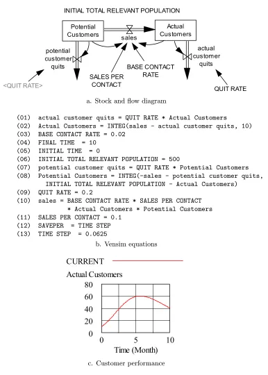
Figure 4.5 shows a process model for a variation on s-shaped growth where the leveling o¯ process is followed by decline. In this process, it is assumed that some Actual Customers and some Potential Customers permanently quit. Such a process might make sense for a new \fad" durable good which comes on the market. In such a situation, there may be a large INITIAL TOTAL RELEVANT POPULATION of possible customers but some of those who purchase the prod-uct and become Actual Customers may lose interest in the prodprod-uct and cease to discuss it with Potential Customers. Similarly, some Potential Customers lose interest before they are contacted by Actual Customers. Gradually both sales and use of the product will decline.

In equation 5 of Figure 4.5, the quitting processes for both Potential Cus-tomers and Actual CusCus-tomers are shown as exponential growth processes running in \reverse." That is, the number of Actual Customers leaving is proportional to the number of Actual Customers rather than the number arriving, as in a standard exponential growth process. Similarly, the number of Potential Cus-tomers leaving is proportional to the number of Potential CusCus-tomers. This type of departure process also can be viewed as a balancing process with a goal of zero, and it is sometimes calledexponential decline or exponential decay. From Figure 4.5c, we see that this exponential decline process eventually leads to a decline in the number of Actual Customers.

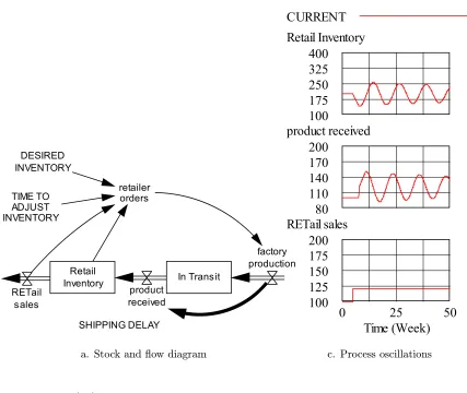
4.5 Oscillating Process

The Figure 4.6a stock and®ow diagram is a simpli±ed version of a production-distribution process. In this process, the retailer orders to the factory depend on both the retail sales and the Retail Inventory level. The factory production process is shown as immediately producing to ful±ll the retailer orders, but there is a delay in the retailer receiving the product because of shipping delays.

In this process, RETail sales are 100 units per week until week 5, at which point they jump to 120 units and remain there for the rest of the simulation run. We see from Figure 4.6c that there are substantial oscillations in key variables of the process.

Unless there are very unusual®ow equations, there must be at least two stocks in a process for the process to oscillate. Furthermore, the degree of oscillation is usually impacted by the delays in the process. The important role of stocks and delays in causing oscillation is one of the factors behind moves to just in time production systems and computer-based ordering processes. These approaches can reduce the stocks in a process and also can reduce delays.

(10)

potential customer

quits

actual customer

quits

QUIT RATE BASE CONTACT

RATE SALES PER

CONTACT

INITIAL TOTAL RELEVANT POPULATION

sales

Actual Customers Potential

Customers

a. Stock and ®ow diagram

(01) actual customer quits = QUIT RATE * Actual Customers

(02) Actual Customers = INTEG(sales - actual customer quits, 10)

(03) BASE CONTACT RATE = 0.02

(06) INITIAL TOTAL RELEVANT POPULATION = 500

(07) potential customer quits = QUIT RATE * Potential Customers

(08) Potential Customers = INTEG(-sales - potential customer quits,

INITIAL TOTAL RELEVANT POPULATION - Actual Customers)

(09) QUIT RATE = 0.2

(10) sales = BASE CONTACT RATE * SALES PER CONTACT

* Actual Customers * Potential Customers

(11) SALES PER CONTACT = 0.1

(13) TIME STEP = 0.0625

b. Vensim equations

CURRENT

Actual Customers

80

60

40

20

0

5

10

Time (Month)

c. Customer performance

(11)

4.5 OSCILLATING PROCESS 39

SHIPPING DELAY TIME TO

ADJUST INVENTORY

DESIRED INVENTORY

retailer orders

factory production

RETail sales

product received

In Transit Retail

Inventory

CURRENT

Retail Inventory

400

325

250

175

100

product received

200

170

140

110

80

RETail sales

200

175

150

125

100

0

25

50

Time (Week)

c. Process oscillations

(01) DESIRED INVENTORY = 200

(02) factory production = retailer orders

(04) In Transit = INTEG(factory production-orders received, 300)

(06) product received = DELAY FIXED(factory production,

SHIPPING DELAY, factory production)

(07) Retail Inventory = INTEG(product received-retail sales, 200)

(08) RETail sales = 100 + STEP(20, 5)

(09) retailer orders = retail sales+ (DESIRED INVENTORY

- Retail Inventory) / TIME TO ADJUST INVENTORY

(11) SHIPPING DELAY = 3

(12) TIME STEP = 0.0625

(13) TIME TO ADJUST INVENTORY = 2

b. Vensim equations

(12)

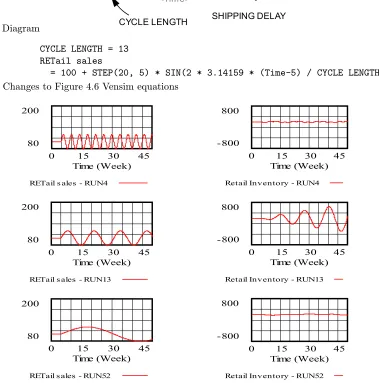
shown in Figure 4.7c. The RUN4 results are for a cycle length of 4 weeks (that is, a monthly cycle). The RUN13 results are for a 13 week (that is, quarterly) cycle, and the RUN52 results are for a 52 week (that is, annual) cycle.

Notice that the amplitude of the variations in Retail Inventory and product received are di¯erent for the three di¯erent cycle lengths. The amplitude is considerably greater for the 13 week cycle than for either the 4 week or 52 week cycles. This is true even though the amplitude of the RETail sales is the same for each cycle length.

Now go back and examine the curves in Figure 4.6c which shows the response of this process to a step change in retail sales. Note in particular that the cycle length for the oscillations is around 12 weeks. A cycle length at which a process oscillates in response to a step input is called a resonance of the process, and the inverse of the cycle length is called a resonant frequency. Thus, a resonant frequency for this process is 1=12 = 0:0833 cycles per week.

A process will generally respond with greater amplitude to inputs which vary with a frequency that is at or near a resonant frequency. Thus, it is to be expected that the response shown in Figure 4.7c for the sinusoidal with a 13 week cycle is greater than the responses for the sinusoids with 4 and 52 week cycles.

In engineered systems, an attempt is often made to keep the resonant frequen-cies considerably di¯erent from the usual variations that are found in operation. This is because of the large responses that such systems typically make to inputs near their resonant frequencies. This can be annoying, or even dangerous. (Have you ever noticed the short period of vibration that some planes go through just after takeo¯? This is a resonance phenomena.)

Unfortunately, the resonant frequencies for many business processes are in the range of variations that are often found in practice. This has two undesirable aspects. First, it means that the amplitude of variations is greater than it might otherwise be. Second, it may lead managers to assume there are external causes for the variations. Suppose that in a particular process these oscillations have periods that are similar to some \natural" time period like a month, quarter, or year. In such a situation, it can be easy to assume that there is some external pattern that has such a period, and start to organize your process to such a cycle. This can make the oscillations worse. For example, consider the traditional yearly cycle in auto sales. Is that due to real variations in consumer demand, or is it created by the way that the auto companies manage their processes?

4.6 References

G. P. Richardson and A. L. Pugh III,Introduction to System Dynamics Modeling with DYNAMO, Productivity Press, Cambridge, Massachusetts, 1981. P. M. Senge, The Fifth Discipline: The Art and Practice of the Learning

(13)

4.6 REFERENCES 41

a. Diagram

<Time>

CYCLE LENGTH SHIPPING DELAY

TIME TO ADJUST INVENTORY DESIRED INVENTORY

retailer orders

factory production

RETail sales

product received

In Transit Retail

Inventory

CYCLE LENGTH = 13 RETail sales

= 100 + STEP(20, 5) * SIN(2 * 3.14159 * (Time-5) / CYCLE LENGTH) b. Changes to Figure 4.6 Vensim equations

200

80

0 15 30 45

Time (Week)

RETail s ales - RUN4

800

-800

0 15 30 45

Time (Week)

Retail Inventory - RUN4

200

80

0 15 30 45

Time (Week)

RETail s ales - RUN13

800

-800

0 15 30 45

Time (Week)

200

80

0 15 30 45

Time (Week)

RETail sales - RUN52

800

-800

0 15 30 45

Time (Week)

c. Process oscillations (4, 13, and 52 week cycles)

(14)