233
CHAPTER
error messages.
—Anonymous
640K [of memory] ought to be enough for anybody.
—Bill Gates
6
Memory
6.1
INTRODUCTION
M
ost computers are built using the Von Neumann model, which is centered onmemory. The programs that perform the processing are stored in memory. We examined a small 4 3-bit memory in Chapter 3 and we learned how to address memory in Chapters 4 and 5. We know memory is logically structured as a linear array of locations, with addresses from 0 to the maximum memory size the processor can address. In this chapter we examine the various types of mem-ory and how each is part of the memmem-ory hierarchy system. We then look at cache memory (a special high-speed memory) and a method that utilizes memory to its fullest by means of virtual memory implemented via paging.6.2
TYPES OF MEMORY
high-performance cache systems. However, before we discuss cache memory, we will explain the various memory technologies.
Even though a large number of memory technologies exist, there are only two basic types of memory: RAM (random access memory) and ROM (read-only memory). RAM is somewhat of a misnomer; a more appropriate name is read-write memory. RAM is the memory to which computer specifications refer; if you buy a computer with 128 megabytes of memory, it has 128MB of RAM. RAM is also the “main memory” we have continually referred to throughout this book. Often called primary memory, RAM is used to store programs and data that the computer needs when executing programs; but RAM is volatile, and loses this information once the power is turned off. There are two general types of chips used to build the bulk of RAM memory in today’s computers: SRAM and DRAM (static and dynamic random access memory).
Dynamic RAM is constructed of tiny capacitors that leak electricity. DRAM requires a recharge every few milliseconds to maintain its data. Static RAM tech-nology, in contrast, holds its contents as long as power is available. SRAM con-sists of circuits similar to the D flip-flops we studied in Chapter 3. SRAM is faster and much more expensive than DRAM; however, designers use DRAM because it is much denser (can store many bits per chip), uses less power, and generates less heat than SRAM. For these reasons, both technologies are often used in combination: DRAM for main memory and SRAM for cache. The basic operation of all DRAM memories is the same, but there are many flavors, includ-ing Multibank DRAM (MDRAM), Fast-Page Mode (FPM) DRAM, Extended Data Out (EDO) DRAM, Burst EDO DRAM (BEDO DRAM), Synchronous Dynamic Random Access Memory (SDRAM), Synchronous-Link (SL) DRAM, Double Data Rate (DDR) SDRAM, and Direct Rambus (DR) DRAM. The differ-ent types of SRAM include asynchronous SRAM, synchronous SRAM, and pipeline burst SRAM. For more information about these types of memory, refer to the references listed at the end of the chapter.
In addition to RAM, most computers contain a small amount of ROM (read-only memory) that stores critical information necessary to operate the system, such as the program necessary to boot the computer. ROM is not volatile and always retains its data. This type of memory is also used in embedded systems or any systems where the programming does not need to change. Many appliances, toys, and most automobiles use ROM chips to maintain information when the power is shut off. ROMs are also used extensively in calculators and peripheral devices such as laser printers, which store their fonts in ROMs. There are five basic different types of ROM: ROM, PROM, EPROM, EEPROM, and flash memory. PROM (programmable read-only memory) is a variation on ROM. PROMs can be programmed by the user with the appropriate equipment. Whereas ROMs are hardwired, PROMs have fuses that can be blown to program the chip. Once programmed, the data and instructions in PROM cannot be changed.
EPROM(erasable PROM) is programmable with the added advantage of being reprogrammable (erasing an EPROM requires a special tool that emits ultraviolet light). To reprogram an EPROM, the entire chip must first be erased. EEPROM
special tools are required for erasure (this is performed by applying an electric field) and you can erase only portions of the chip, one byte at a time. Flash mem-ory is essentially EEPROM with the added benefit that data can be written or erased in blocks, removing the one-byte-at-a-time limitation. This makes flash memory faster than EEPROM.
6.3
THE MEMORY HIERARCHY
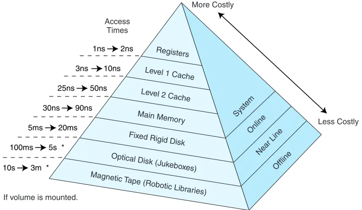
One of the most important considerations in understanding the performance capa-bilities of a modern processor is the memory hierarchy. Unfortunately, as we have seen, not all memory is created equal, and some types are far less efficient and thus cheaper than others. To deal with this disparity, today’s computer systems use a combination of memory types to provide the best performance at the best cost. This approach is called hierarchical memory. As a rule, the faster memory is, the more expensive it is per bit of storage. By using a hierarchy of memories, each with different access speeds and storage capacities, a computer system can exhibit performance above what would be possible without a combination of the various types. The base types that normally constitute the hierarchical memory system include registers, cache, main memory, and secondary memory.
Today’s computers each have a small amount of very high-speed memory, called a cache, where data from frequently used memory locations may be tem-porarily stored. This cache is connected to a much larger main memory, which is typically a medium-speed memory. This memory is complemented by a very large secondary memory, composed of a hard disk and various removable media. By using such a hierarchical scheme, one can improve the effective access speed of the memory, using only a small number of fast (and expensive) chips. This allows designers to create a computer with acceptable performance at a reason-able cost.
We classify memory based on its “distance” from the processor, with distance measured by the number of machine cycles required for access. The closer mem-ory is to the processor, the faster it should be. As memmem-ory gets further from the main processor, we can afford longer access times. Thus, slower technologies are used for these memories, and faster technologies are used for memories closer to the CPU. The better the technology, the faster and more expensive the memory becomes. Thus, faster memories tend to be smaller than slower ones, due to cost.
The following terminology is used when referring to this memory hierarchy:
• Hit—The requested data resides in a given level of memory (typically, we are concerned with the hit rate only for upper levels of memory).
• Miss—The requested data is not found in the given level of memory.
• Hit rate—The percentage of memory accesses found in a given level of memory. • Miss rate—The percentage of memory accesses not found in a given level of
memory. Note: Miss Rate = 1 Hit Rate.
Magnetic
Tape (Robotic Libr aries) Optical Disk (J
ukeboxes) Fixed Rigid Disk
Main Memor y Level 2 Cache
Level 1 Cache Registers
Offline Near Line Online System More Costly
Access Times
Less Costly 1ns 2ns
3ns 10ns
25ns 50ns
30ns 90ns
5ms 20ms
100ms 5s *
10s 3m *
* If volume is mounted.
FIGURE 6.1 The Memory Hierarchy
• Miss penalty—The time required to process a miss, which includes replacing a block in an upper level of memory, plus the additional time to deliver the requested data to the processor. (The time to process a miss is typically signifi-cantly larger than the time to process a hit.)
The memory hierarchy is illustrated in Figure 6.1. This is drawn as a pyramid to help indicate the relative sizes of these various memories. Memories closer to the top tend to be smaller in size. However, these smaller memories have better per-formance and thus a higher cost (per bit) than memories found lower in the pyra-mid. The numbers given to the left of the pyramid indicate typical access times.
cache, for X, there may be several hits in cache on the newly retrieved block afterward, due to locality.
6.3.1 Locality of Reference
In practice, processors tend to access memory in a very patterned way. For exam-ple, in the absence of branches, the PC in MARIE is incremented by one after each instruction fetch. Thus, if memory location Xis accessed at time t, there is a high probability that memory location X + 1 will also be accessed in the near future. This clustering of memory references into groups is an example of locality of reference. This locality can be exploited by implementing the memory as a hierarchy; when a miss is processed, instead of simply transferring the requested data to a higher level, the entire block containing the data is transferred. Because of locality of reference, it is likely that the additional data in the block will be needed in the near future, and if so, this data can be loaded quickly from the faster memory.
There are three basic forms of locality:
• Temporal locality—Recently accessed items tend to be accessed again in the near future.
• Spatial locality—Accesses tend to be clustered in the address space (for exam-ple, as in arrays or loops).
• Sequential locality—Instructions tend to be accessed sequentially.
The locality principle provides the opportunity for a system to use a small amount of very fast memory to effectively accelerate the majority of memory accesses. Typically, only a small amount of the entire memory space is being accessed at any given time, and values in that space are being accessed repeatedly. Therefore, we can copy those values from a slower memory to a smaller but faster memory that resides higher in the hierarchy. This results in a memory system that can store a large amount of information in a large but low-cost memory, yet provide nearly the same access speeds that would result from using very fast but expensive memory.
6.4
CACHE MEMORY
A computer processor is very fast and is constantly reading information from memory, which means it often has to wait for the information to arrive, because the memory access times are slower than the processor speed. A cache memory is a small, temporary, but fast memory that the processor uses for information it is likely to need again in the very near future.
the tape measure from a huge tool storage chest, run down to the basement, meas-ure the wood, run back out to the garage, leave the tape measmeas-ure, grab the saw, and then return to the basement with the saw and cut the wood. Now you decide to bolt some pieces of wood together. So you run to the garage, grab the drill set, go back down to the basement, drill the holes to put the bolts through, go back to the garage, leave the drill set, grab one wrench, go back to the basement, find out the wrench is the wrong size, go back to the tool chest in the garage, grab another wrench, run back downstairs . . . wait! Would you really work this way? No! Being a reasonable person, you think to yourself “If I need one wrench, I will probably need another one of a different size soon anyway, so why not just grab the whole set of wrenches?” Taking this one step further, you reason “Once I am done with one certain tool, there is a good chance I will need another soon, so why not just pack up a small toolbox and take it to the basement?” This way, you keep the tools you need close at hand, so access is faster. You have just cached some tools for easy access and quick use! The tools you are less likely to use remain stored in a location that is further away and requires more time to access. This is all that cache memory does: It stores data that has been accessed and data that might be accessed by the CPU in a faster, closer memory.
Another cache analogy is found in grocery shopping. You seldom, if ever, go to the grocery store to buy one single item. You buy any items you require imme-diately in addition to items you will most likely use in the future. The grocery store is similar to main memory, and your home is the cache. As another example, consider how many of us carry around an entire phone book. Most of us have a small address book instead. We enter the names and numbers of people we tend to call more frequently; looking a number up in our address book is much quicker than finding a phone book, locating the name, and then getting the number. We tend to have the address book close at hand, whereas the phone book is probably located in our home, hidden in an end table or bookcase somewhere. The phone book is something we do not use frequently, so we can afford to store it in a little more out of the way location. Comparing the size of our address book to the tele-phone book, we see that the address book “memory” is much smaller than that of a telephone book. But the probability is very high that when we make a call, it is to someone in our address book.
Students doing research offer another commonplace cache example. Suppose you are writing a paper on quantum computing. Would you go to the library, check out one book, return home, get the necessary information from that book, go back to the library, check out another book, return home, and so on? No, you would go to the library and check out all the books you might need and bring them all home. The library is analogous to main memory, and your home is, again, similar to cache.
desk. The filing cabinets are her “main memory” and her desk (with its many unorganized-looking piles) is the cache.
Cache memory works on the same basic principles as the preceding examples by copying frequently used data into the cache rather than requiring an access to main memory to retrieve the data. Cache can be as unorganized as your author’s desk or as organized as your address book. Either way, however, the data must be accessible (locatable). Cache memory in a computer differs from our real-life examples in one important way: The computer really has no way to know, a pri-ori, what data is most likely to be accessed, so it uses the locality principle and transfers an entire block from main memory into cache whenever it has to make a main memory access. If the probability of using something else in that block is high, then transferring the entire block saves on access time. The cache location for this new block depends on two things: the cache mapping policy (discussed in the next section) and the cache size (which affects whether there is room for the new block).
The size of cache memory can vary enormously. A typical personal com-puter’s level 2 (L2) cache is 256K or 512K. Level 1 (L1) cache is smaller, typi-cally 8K or 16K. L1 cache resides on the processor, whereas L2 cache resides between the CPU and main memory. L1 cache is, therefore, faster than L2 cache. The relationship between L1 and L2 cache can be illustrated using our grocery store example: If the store is main memory, you could consider your refrigerator the L2 cache, and the actual dinner table the L1 cache.
The purpose of cache is to speed up memory accesses by storing recently used data closer to the CPU, instead of storing it in main memory. Although cache is not as large as main memory, it is considerably faster. Whereas main memory is typically composed of DRAM with, say, a 60ns access time, cache is typically composed of SRAM, providing faster access with a much shorter cycle time than DRAM (a typical cache access time is 10ns). Cache does not need to be very large to perform well. A general rule of thumb is to make cache small enough so that the overall average cost per bit is close to that of main memory, but large enough to be beneficial. Because this fast memory is quite expensive, it is not feasible to use the technology found in cache memory to build all of main memory.
What makes cache “special”? Cache is not accessed by address; it is accessed by content. For this reason, cache is sometimes calledcontent addressable memory
orCAM. Under most cache mapping schemes, the cache entries must be checked or searched to see if the value being requested is stored in cache. To simplify this process of locating the desired data, various cache mapping algorithms are used.
6.4.1 Cache Mapping Schemes
first location in cache. How, then, does the CPU locate data when it has been copied into cache? The CPU uses a specific mapping scheme that “converts” the main memory address into a cache location.
This address conversion is done by giving special significance to the bits in the main memory address. We first divide the bits into distinct groups we call
fields. Depending on the mapping scheme, we may have two or three fields. How we use these fields depends on the particular mapping scheme being used. The mapping scheme determines where the data is placed when it is originally copied into cache and also provides a method for the CPU to find previously copied data when searching cache.
Before we discuss these mapping schemes, it is important to understand how data is copied into cache. Main memory and cache are both divided into the same size blocks (the size of these blocks varies). When a memory address is gener-ated, cache is searched first to see if the required word exists there. When the requested word is not found in cache, the entire main memory block in which the word resides is loaded into cache. As previously mentioned, this scheme is suc-cessful because of the principle of locality—if a word was just referenced, there is a good chance words in the same general vicinity will soon be referenced as well. Therefore, one missed word often results in several found words. For exam-ple, when you are in the basement and you first need tools, you have a “miss” and must go to the garage. If you gather up a set of tools that you might need and return to the basement, you hope that you’ll have several “hits” while working on your home improvement project and don’t have to make many more trips to the garage. Because accessing a cache word (a tool already in the basement) is faster than accessing a main memory word (going to the garage yet again!), cache mem-ory speeds up the overall access time.
So, how do we use fields in the main memory address? One field of the main memory address points us to a location in cache in which the data resides if it is resident in cache (this is called acache hit), or where it is to be placed if it is not resident (which is called a cache miss). (This is slightly different for associative mapped cache, which we discuss shortly.) The cache block refer-enced is then checked to see if it is valid. This is done by associating a valid bit
with each cache block. A valid bit of 0 means the cache block is not valid (we have a cache miss) and we must access main memory. A valid bit of 1 means it is valid (we may have a cache hit but we need to complete one more step before we know for sure). We then compare the tag in the cache block to the tag field
Direct Mapped Cache
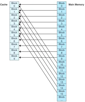
Direct mapped cache assigns cache mappings using a modular approach. Because there are more main memory blocks than there are cache blocks, it should be clear that main memory blocks compete for cache locations. Direct mapping maps block Xof main memory to block Y of cache, mod N, where Nis the total number of blocks in cache. For example, if cache contains 10 blocks, then main memory block 0 maps to cache block 0, main memory block 1 maps to cache block 1, . . . , main memory block 9 maps to cache block 9, and main memory block 10 maps to cache block 0. This is illustrated in Figure 6.2. Thus, main memory blocks 0 and 10 (and 20, 30, and so on) all compete for cache block 0.
You may be wondering, if main memory blocks 0 and 10 both map to cache block 0, how does the CPU know which block actually resides in cache block 0 at any given time? The answer is that each block is copied to cache and identified
Block 0 Block
1 Block
2 Block
3 Block
4 Block
5 Block
6 Block
7 Block
8 Block
9
Block 0 Block
1 Block
2 Block
3 Block
4 Block
5 Block
6 Block
7 Block
8 Block
9 Block
10 Block
11 Block
12 Block
13 Block
14 Block
15 Block
...
Cache Main Memory
11110101
00000000 words A, B, C,... words L, M, N,...
---Tag
Block Data Valid
1 1
0 0 0
1
2 3
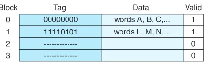
FIGURE 6.3 A Closer Look at Cache
by the tag previously described. If we take a closer look at cache, we see that it stores more than just that data copied from main memory, as indicated in Figure 6.3. In this figure, there are two valid cache blocks. Block 0 contains multiple words from main memory, identified using the tag “00000000”. Block 1 contains words identified using tag “11110101”. The other two cache blocks are not valid.
To perform direct mapping, the binary main memory address is partitioned into the fields shown in Figure 6.4.
The size of each field depends on the physical characteristics of main mem-ory and cache. The wordfield (sometimes called the offsetfield) uniquely identi-fies a word from a specific block; therefore, it must contain the appropriate number of bits to do this. This is also true of the block field—it must select a unique block of cache. The tag field is whatever is left over. When a block of main memory is copied to cache, this tag is stored with the block and uniquely identifies this block. The total of all three fields must, of course, add up to the number of bits in a main memory address.
Consider the following example: Assume memory consists of 214 words,
cache has 16 blocks, and each block has 8 words. From this we determine that
memory has 2
14
23 =2
11 blocks. We know that each main memory address requires
14 bits. Of this 14-bit address field, the rightmost 3 bits reflect the word field (we need 3 bits to uniquely identify one of 8 words in a block). We need 4 bits to select a specific block in cache, so the block field consists of the middle 4 bits. The remaining 7 bits make up the tag field. The fields with sizes are illustrated in Figure 6.5.
As mentioned previously, the tag for each block is stored with that block in the cache. In this example, because main memory blocks 0 and 16 both map to cache block 0, the tag field would allow the system to differentiate between block
Tag Block Word
Bits in Main Memory Address
Tag Block Word
1 bit 2 bits 1 bit
4 bits
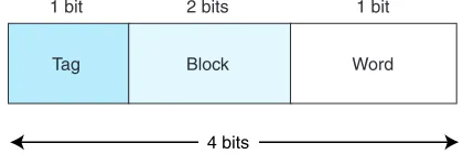
FIGURE 6.6 The Main Memory Address Format for a 16-Word Memory
Tag Block Word
7 bits 4 bits 3 bits
14 bits
FIGURE 6.5 The Main Memory Address Format for Our Example
0 and block 16. The binary addresses in block 0 differ from those in block 16 in the upper leftmost 7 bits, so the tags are different and unique.
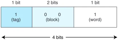
To see how these addresses differ, let’s look at a smaller, simpler example. Suppose we have a system using direct mapping with 16 words of main memory divided into 8 blocks (so each block has 2 words). Assume the cache is 4 blocks in size (for a total of 8 words). Table 6.1 shows how the main memory blocks map to cache.
We know:
• A main memory address has 4 bits (because there are 24 or 16 words in
main memory).
• This 4-bit main memory address is divided into three fields: The word field is 1 bit (we need only 1 bit to differentiate between the two words in a block); the block field is 2 bits (we have 4 blocks in main memory and need 2 bits to uniquely iden-tify each block); and the tag field has 1 bit (this is all that is left over).
The main memory address is divided into the fields shown in Figure 6.6.
TABLE 6.1 An Example of Main Memory Mapped to Cache
1 (tag)
0 0 (block)
1 (word)
1 bit 2 bits 1 bit
4 bits
FIGURE 6.7 The Main Memory Address 9 = 10012Split into Fields
Suppose we generate the main memory address 9. We can see from the map-ping listing above that address 9 is in main memory block 4 and should map to cache block 0 (which means the contents of main memory block 4 should be copied into cache block 0). The computer, however, uses the actual main memory address to determine the cache mapping block. This address, in binary, is repre-sented in Figure 6.7.
When the CPU generates this address, it first takes the block field bits 00 and uses these to direct it to the proper block in cache. 00 indicates that cache block 0 should be checked. If the cache block is valid, it then compares the tag field value of 1 (in the main memory address) to the tag associated with cache block 0. If the cache tag is 1, then block 4 currently resides in cache block 0. If the tag is 0, then block 0 from main memory is located in block 0 of cache. (To see this, compare main memory address 9 = 10012, which is in block 4, to main memory address 1 = 00012, which is in block 0. These two addresses differ only in the leftmost bit, which is the bit used as the tag by the cache.) Assuming the tags match, which means that block 4 from main memory (with addresses 8 and 9) resides in cache block 0, the word field value of 1 is used to select one of the two words residing in the block. Because the bit is 1, we select the word with offset 1, which results in retrieving the data copied from main memory address 9.
Let’s do one more example in this context. Suppose the CPU now generates address 4 = 01002. The middle two bits (10) direct the search to cache block 2. If the block is valid, the leftmost tag bit (0) would be compared to the tag bit stored with the cache block. If they match, the first word in that block (of offset 0) would be returned to the CPU. To make sure you understand this process, per-form a similar exercise with the main memory address 12 = 11002.
Let’s move on to a larger example. Suppose we have a system using 15-bit main memory addresses and 64 blocks of cache. If each block contains 8 words, we know that the main memory 15-bit address is divided into a 3-bit word field, a 6-bit block field, and a 6-bit tag field. If the CPU generates the main memory address:
000010
1028 = 000000 100
Tag Word
11 bits 3 bits
14 bits
FIGURE 6.8 The Main Memory Address Format for Associative Mapping
it would look in block 0 of cache, and if it finds a tag of 000010, the word at off-set 4 in this block would be returned to the CPU.
Fully Associative Cache
Direct mapped cache is not as expensive as other caches because the mapping scheme does not require any searching. Each main memory block has a specific location to which it maps in cache; when a main memory address is converted to a cache address, the CPU knows exactly where to look in the cache for that mem-ory block by simply examining the bits in the block field. This is similar to your address book: The pages often have an alphabetic index, so if you are searching for “Joe Smith,” you would look under the “s” tab.
Instead of specifying a unique location for each main memory block, we can look at the opposite extreme: allowing a main memory block to be placed any-where in cache. The only way to find a block mapped this way is to search all of cache. (This is similar to your author’s desk!) This requires the entire cache to be built fromassociative memoryso it can be searched in parallel. That is, a single search must compare the requested tag toall tags in cache to determine whether the desired data block is present in cache. Associative memory requires special hardware to allow associative searching, and is, thus, quite expensive.
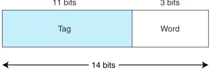
Using associative mapping, the main memory address is partitioned into two pieces, the tag and the word. For example, using our previous memory configura-tion with 214words, a cache with 16 blocks, and blocks of 8 words, we see from
Figure 6.8 that the word field is still 3 bits, but now the tag field is 11 bits. This tag must be stored with each block in cache. When the cache is searched for a specific main memory block, the tag field of the main memory address is compared to all the valid tag fields in cache; if a match is found, the block is found. (Remember, the tag uniquely identifies a main memory block.) If there is no match, we have a cache miss and the block must be transferred from main memory.
would a least-recently used algorithm. There are many replacement algorithms that can be used; these are discussed shortly.
Set Associative Cache
Owing to its speed and complexity, associative cache is very expensive. Although direct mapping is inexpensive, it is very restrictive. To see how direct mapping limits cache usage, suppose we are running a program on the architecture described in our previous examples. Suppose the program is using block 0, then block 16, then 0, then 16, and so on as it executes instructions. Blocks 0 and 16 both map to the same location, which means the program would repeatedly throw out 0 to bring in 16, then throw out 16 to bring in 0, even though there are addi-tional blocks in cache not being used. Fully associative cache remedies this prob-lem by allowing a block from main memory to be placed anywhere. However, it requires a larger tag to be stored with the block (which results in a larger cache) in addition to requiring special hardware for searching of all blocks in cache simultaneously (which implies a more expensive cache). We need a scheme somewhere in the middle.
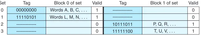
The third mapping scheme we introduce is N-way set associative cache map-ping, a combination of these two approaches. This scheme is similar to direct mapped cache, in that we use the address to map the block to a certain cache loca-tion. The important difference is that instead of mapping to a single cache block, an address maps to a set of several cache blocks. All sets in cache must be the same size. This size can vary from cache to cache. For example, in a 2-way set associative cache, there are two cache blocks per set, as seen in Figure 6.9. In this figure, we see that set 0 contains two blocks, one that is valid and holds the data A, B, C, . . . , and another that is not valid. The same is true for Set 1. Set 2 and Set 3 can also hold two blocks, but currently, only the second block is valid in each set. In an 8-way set associative cache, there are 8 cache blocks per set. Direct mapped cache is a special case of N-way set associative cache mapping where the set size is one.
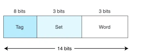
In set-associative cache mapping, the main memory address is partitioned into three pieces: the tag field, the set field, and the word field. The tag and word fields assume the same roles as before; the set field indicates into which cache set the main memory block maps. Suppose we are using 2-way set associative map-ping with a main memory of 214words, a cache with 16 blocks, where each block
contains 8 words. If cache consists of a total of 16 blocks, and each set has 2
11110101
00000000 Words A, B, C, . . . Words L, M, N, . . .
---Tag
Set Block 0 of set Valid
1 1
0 10111011 P, Q, R, . . .
---Tag Block 1 of set Valid
0 0
1 0
1
2
--- 0 11111100 T, U, V, . . . 1 3
Tag Set Word 8 bits 3 bits 3 bits
14 bits
FIGURE 6.10 Format for Set Associative Mapping
blocks, then there are 8 sets in cache. Therefore, the set field is 3 bits, the word field is 3 bits, and the tag field is 8 bits. This is illustrated in Figure 6.10.
6.4.2 Replacement Policies
In a direct-mapped cache, if there is contention for a cache block, there is only one possible action: The existing block is kicked out of cache to make room for the new block. This process is called replacement. With direct mapping, there is no need for a replacement policy because the location for each new block is pre-determined. However, with fully associative cache and set associative cache, we need a replacement algorithm to determine the “victim” block to be removed from cache. When using fully associative cache, there are Kpossible cache loca-tions (where Kis the number of blocks in cache) to which a given main memory block may map. With N-way set associative mapping, a block can map to any of
Ndifferent blocks within a given set. How do we determine which block in cache should be replaced? The algorithm for determining replacement is called the
replacement policy.
There are several popular replacement policies. One that is not practical but that can be used as a benchmark by which to measure all others is the optimal
algorithm. We like to keep values in cache that will be needed again soon, and throw out blocks that won’t be needed again, or that won’t be needed for some time. An algorithm that could look into the future to determine the precise blocks to keep or eject based on these two criteria would be best. This is what the optimal algorithm does. We want to replace the block that will not be used for the longest period of time in the future. For example, if the choice for the victim block is between block 0 and block 1, and block 0 will be used again in 5 seconds, whereas block 1 will not be used again for 10 seconds, we would throw out block 1. From a practical standpoint, we can’t look into the future—but we can run a program and then rerun it, so we effectivelydoknow the future. We can then apply the optimal algorithm on the second run. The optimal algorithm guarantees the lowest possi-ble miss rate. Because we cannot see the future on every single program we run, the optimal algorithm is used only as a metric to determine how good or bad another algorithm is. The closer an algorithm performs to the optimal algorithm, the better.
soon. We can keep track of the last time each block was accessed (assign a time-stamp to the block), and select as the victim block the block that has been used least recently. This is the least recently used (LRU) algorithm. Unfortunately, LRU requires the system to keep a history of accesses for every cache block, which requires significant space and slows down the operation of the cache. There are ways to approximate LRU, but that is beyond the scope of this book. (Refer to the references at the end of the chapter for more information.)
First in, first out (FIFO) is another popular approach. With this algorithm, the block that has been in cache the longest (regardless of how recently it has been used) would be selected as the victim to be removed from cache memory.
Another approach is to select a victim atrandom. The problem with LRU and FIFO is that there are degenerate referencing situations in which they can be made to
thrash(constantly throw out a block, then bring it back, then throw it out, then bring it back, repeatedly). Some people argue that random replacement, although it some-times throws out data that will be needed soon, never thrashes. Unfortunately, it is difficult to have truly random replacement, and it can decrease average performance. The algorithm selected often depends on how the system will be used. No single (practical) algorithm is best for all scenarios. For that reason, designers use algorithms that perform well under a wide variety of circumstances.
6.4.3 Effective Access Time and Hit Ratio
The performance of a hierarchical memory is measured by its effective access time(EAT), or the average time per access. EAT is a weighted average that uses the hit ratio and the relative access times of the successive levels of the hierarchy. For example, suppose the cache access time is 10ns, main memory access time is 200ns, and the cache hit rate is 99%. The average time for the processor to access an item in this two-level memory would then be:
What, exactly, does this mean? If we look at the access times over a long period of time, this system performs as if it had a single large memory with an 11ns access time. A 99% cache hit rate allows the system to perform very well, even though most of the memory is built using slower technology with an access time of 200ns. The formula for calculating effective access time for a two-level memory is given by:
EAT = HAccessC+ (1 H) AccessMM
where H = cache hit rate, AccessC= cache access time, and AccessMM = main memory access time.
This formula can be extended to apply to three- or even four-level memories, as we will see shortly.
EAT = 0.99(10ns) + 0.01(200ns) = 9.9ns + 2ns = 11ns
6.4.4 When Does Caching Break Down?
When programs exhibit locality, caching works quite well. However, if programs exhibit bad locality, caching breaks down and the performance of the memory hierar-chy is poor. In particular, object-oriented programming can cause programs to exhibit less than optimal locality. Another example of bad locality can be seen in two-dimen-sional array access. Arrays are typically stored in row-major order. Suppose, for pur-poses of this example, that one row fits exactly in one cache block and cache can hold all but one row of the array. If a program accesses the array one row at a time, the first row access produces a miss, but once the block is transferred into cache, all subse-quent accesses to that row are hits. So a 54 array would produce 5 misses and 15 hits over 20 accesses (assuming we are accessing each element of the array). If a pro-gram accesses the array in column-major order, the first access to the column results in a miss, after which an entire row is transferred in. However, the second access to the column results in another miss. The data being transferred in for each row is not being used because the array is being accessed by column. Because cache is not large enough, this would produce 20 misses on 20 accesses. A third example would be a program that loops through a linear array that does not fit in cache. There would be a significant reduction in the locality when memory is used in this fashion.
6.4.5 Cache Write Policies
In addition to determining which victim to select for replacement, designers must also decide what to do with so-called dirty blocks of cache, or blocks that have been modified. When the processor writes to main memory, the data may be writ-ten to the cache instead under the assumption that the processor will probably read it again soon. If a cache block is modified, the cache write policydetermines when the actual main memory block is updated to match the cache block. There are two basic write policies:
• Write-through—A write-through policy updates both the cache and the main memory simultaneously on every write. This is slower than write-back, but ensures that the cache is consistent with the main system memory. The obvious disadvantage here is that every write now requires a main memory access. Using a write-through policy means every write to the cache necessitates a main memory write, thus slowing the system (if all accesses are write, this essentially slows the system down to main memory speed). However, in real applications, the majority of accesses are reads so this slow-down is negligible. • Write-back—A write-back policy (also calledcopyback) only updates blocks in main memory when the cache block is selected as a victim and must be removed from cache. This is normally faster than write-through because time is not wasted writing information to memory on each write to cache. Memory traffic is also reduced. The disadvantage is that main memory and cache may not contain the same value at a given instant of time, and if a process terminates (crashes) before the write to main memory is done, the data in cache may be lost.
write operations (potentially a 15% increase), better replacement algorithms (up to a 10% increase), and better coding practices, as we saw in the earlier example of row versus column-major access (up to a 30% increase in hit ratio). Simply increasing the size of cache may improve the hit ratio by roughly 1–4%, but is not guaranteed to do so.
6.5
VIRTUAL MEMORY
You now know that caching allows a computer to access frequently used data from a smaller but faster cache memory. Cache is found near the top of our mem-ory hierarchy. Another important concept inherent in the hierarchy is virtual memory. The purpose of virtual memory is to use the hard disk as an extension of RAM, thus increasing the available address space a process can use. Most per-sonal computers have a relatively small amount (typically less than 512MB) of main memory. This is usually not enough memory to hold multiple applications concurrently, such as a word processing application, an e-mail program, and a graphics program, in addition to the operating system itself. Using virtual mem-ory, your computer addresses more main memory than it actually has, and it uses the hard drive to hold the excess. This area on the hard drive is called a page file, because it holds chunks of main memory on the hard drive. The easiest way to think about virtual memory is to conceptualize it as an imaginary memory loca-tion in which all addressing issues are handled by the operating system.
The most common way to implement virtual memory is by using paging, a method in which main memory is divided into fixed-size blocks and programs are divided into the same size blocks. Typically, chunks of the program are brought into memory as needed. It is not necessary to store contiguous chunks of the program in contiguous chunks of main memory. Because pieces of the program can be stored out of order, program addresses, once generated by the CPU, must be translated to main memory addresses. Remember, in caching, a main memory address had to be transformed into a cache location. The same is true when using virtual memory; every virtual address must be translated into a physical address. How is this done? Before delving further into an explanation of virtual memory, let’s define some fre-quently used terms for virtual memory implemented through paging:
• Virtual address—The logical or program address that the process uses. When-ever the CPU generates an address, it is always in terms of virtual address space. • Physical address—The real address in physical memory.
• Mapping—The mechanism by which virtual addresses are translated into physical ones (very similar to cache mapping)
• Page frames—The equal-size chunks or blocks into which main memory
(physical memory) is divided.
• Paging—The process of copying a virtual page from disk to a page frame in main memory.
• Fragmentation—Memory that becomes unusable.
• Page fault—An event that occurs when a requested page is not in main mem-ory and must be copied into memmem-ory from disk.
Because main memory and virtual memory are divided into equal size pages, pieces of the process address space can be moved into main memory but need not be stored contiguously. As previously stated, we need not have all of the process in main memory at once; virtual memory allows a program to run when only spe-cific pieces are present in memory. The parts not currently being used are stored in the page file on disk.
Virtual memory can be implemented with different techniques, including paging, segmentation, or a combination of both, but paging is the most popular. (This topic is covered in great detail within the study of operating systems.) The success of paging, like that of cache, is very dependent on the locality principle. When data is needed that does not reside in main memory, the entire block in which it resides is copied from disk to main memory, in hopes that other data on the same page will be useful as the program continues to execute.
6.5.1 Paging
The basic idea behind paging is quite simple: Allocate physical memory to processes in fixed size chunks (page frames) and keep track of where the various pages of the process reside by recording information in a page table. Every process has its own page table that typically resides in main memory, and the page table stores the physical location of each virtual page of the process. The page table has Nrows, where Nis the number of virtual pages in the process. If there are pages of the process currently not in main memory, the page table indi-cates this by setting a valid bitto 0; if the page is in main memory, the valid bit is set to 1. Therefore, each entry of the page table has two fields: a valid bit and a frame number.
Additional fields are often added to relay more information. For example, a
dirty bit (or amodify bit) could be added to indicate whether the page has been changed. This makes returning the page to disk more efficient, because if it is not modified, it does not need to be rewritten to disk. Another bit (theusage bit) can be added to indicate the page usage. This bit is set to 1 whenever the page is accessed. After a certain time period, the usage bit is set to 0. If the page is refer-enced again, the usage bit is set to 1. However, if the bit remains 0, this indicates that the page has not been used for a period of time, and the system might benefit by sending this page out to disk. By doing so, the system frees up this page’s location for another page that the process eventually needs (we discuss this in more detail when we introduce replacement algorithms).
actually need the entire page frame, but no other process may use it. Therefore, the unused memory in this last frame is effectively wasted. It might happen that the process itself requires less than one page in its entirety, but it must occupy an entire page frame when copied to memory. Internal fragmentation is unusable space withina given partition (in this case, a page) of memory.
Now that you understand what paging is, we will discuss how it works. When a process generates a virtual address, the operating system must dynamically translate this virtual address into the physical address in memory at which the data actually resides. (For purposes of simplicity, let’s assume we have no cache memory for the moment.) For example, from a program viewpoint, we see the final byte of a 10-byte program as address 9, assuming byte instructions and 1-byte addresses, and a starting address of 0. However, when actually loaded into memory, the logical address 9 (perhaps a reference to the label Xin an assembly language program) may actually reside in physical memory location 1239, imply-ing the program was loaded startimply-ing at physical address 1230. There must be an easy way to convert the logical, or virtual, address 9 to the physical address 1230. To accomplish this address translation, a virtual address is divided into two fields: apage fieldand anoffset field, to represent the offset within that page where the requested data is located. This address translation process is similar to the process we used when we divided main memory addresses into fields for the cache mapping algorithms. And similar to cache blocks, page sizes are usually powers of 2; this simplifies the extraction of page numbers and offsets from virtual addresses. To access data at a given virtual address, the system performs the following steps:
1. Extract the page number from the virtual address. 2. Extract the offset from the virtual address.
3. Translate the page number into a physical page frame number by accessing the page table.
A. Look up the page number in the page table (using the virtual page number as an index).
B. Check the valid bit for that page.
1. If the valid bit = 0, the system generates a page fault and the operating system must intervene to
a. Locate the desired page on disk.
b. Find a free page frame (this may necessitate removing a “victim” page from memory and copying it back to disk if memory is full). c. Copy the desired page into the free page frame in main memory. d. Update the page table. (The virtual page just brought in must have its
frame number and valid bit in the page table modified. If there was a “victim” page, its valid bit must be set to zero.)
0
1
2
3
0
1
2
3
4
5
6
7
Virtual Memory Physical Memory
2 -0 1 -3
1 0 0 1 1 0 0 1 0
1 2 3 4 5 6 7
Frame # Valid Bit Page Table Page
FIGURE 6.11 Current State Using Paging and the Associated Page Table
2. If the valid bit = 1, the page is in memory.
a. Replace the virtual page number with the actual frame number. b. Access data at offset in physical page frame by adding the offset to
the frame number for the given virtual page.
Please note that if a process has free frames in main memory when a page fault occurs, the newly retrieved page can be placed in any of those free frames. How-ever, if the memory allocated to the process is full, a victim page must be selected. The replacement algorithms used to select a victim are quite similar to those used in cache. FIFO, Random, and LRU are all potential replacement rithms for selecting a victim page. (For more information on replacement algo-rithms, see the references at the end of this chapter.)
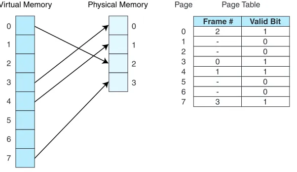
Let’s look at an example. Suppose that we have a virtual address space of 28
words for a given process (this means the program generates addresses in the range 0 to 25510which is 00 to FF16), and physical memory of 4 page frames (no cache). Assume also that pages are 32 words in length. Virtual addresses contain 8 bits, and physical addresses contain 7 bits (4 frames of 32 words each is 128 words, or 27). Suppose, also, that some pages from the process have been brought
into main memory. Figure 6.11 illustrates the current state of the system.
Each virtual address has 8 bits and is divided into 2 fields: the page field has
3 bits, indicating there are 23pages of virtual memory
2825
=
2
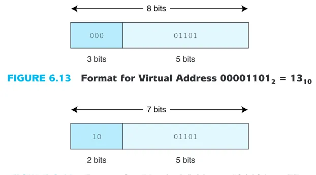
3. Each page is 25= 32 words in length, so we need 5 bits for the page offset. Therefore, an 8-bitvirtual address has the format shown in Figure 6.12.
Page Offset
3 bits 5 bits 8 bits
FIGURE 6.12 Format for an 8-Bit Virtual Address with 25= 32 Word Page Size
6.13), we see the page field P = 0002and the offset field equals 011012. To con-tinue the translation process, we use the 000 value of the page field as an index into the page table. Going to the 0th entry in the page table, we see that virtual page 0 maps to physical page frame 2 = 102. Thus the translated physical address becomes page frame 2, offset 13. Note that a physical address has only 7 bits (2 for the frame, because there are 4 frames, and 5 for the offset). Written in binary, using the two fields, this becomes 10011012, or address 4D16= 7710and is shown in Figure 6.14. We can also find this address another way. Each page has 32 words. We know the virtual address we want is on virtual page 0, which maps to physical page frame 2. Frame 2 begins with address 64. An offset of 13 results in address 77.
Let’s look at a complete example in a real (but small) system (again, with no cache). Suppose a program is 16 bytes long, has access to an 8-byte memory that uses byte addressing (this means each byte, or word, has its own address), and a page is 2 words (bytes) in length. As the program executes, it generates the fol-lowing address reference string (addresses are given in decimal values): 0, 1, 2, 3, 6, 7, 10, 11. (This address reference string indicates that address 0 is referenced first, then address 1, then address 2, and so on.) Originally, memory contains no pages for this program. When address 0 is needed, both address 0 and address 1 (in page 0) are copied to page frame 2 in main memory (it could be that frames 0
000 01101
3 bits 5 bits 8 bits
FIGURE 6.13 Format for Virtual Address 000011012= 1310
10 01101
2 bits 5 bits 7 bits
and 1 of memory are occupied by another process and thus unavailable). This is an example of a page fault, because the desired page of the program had to be fetched from disk. When address 1 is referenced, the data already exists in mem-ory (so we have a page hit). When address 2 is referenced, this causes another page fault, and page 1 of the program is copied to frame 0 in memory. This con-tinues, and after these addresses are referenced and pages are copied from disk to main memory, the state of the system is as shown in Figure 6.15a. We see that address 0 of the program, which contains the data value “A”, currently resides in
A B C D E F G H I J K L M N O P
0 = 0000 1 = 0001 2 = 0010 3 = 0011 4 = 0100 5 = 0101 6 = 0110 7 = 0111
0 = 000 1 = 001 2 = 010 3 = 011 4 = 100 5 = 101 6 = 110 7 = 111 8 = 1000
9 = 1001 10 = 1010 11 = 1011 12 = 1100 13 = 1101 14 = 1110 15 = 1111
C D G H A B K L
a. Program Address Space
Main Memory Address Page 0
1 2 3 4 5 6 7 Page Frame 0
b. Page Table c. Virtual Address 1010 = 10102
4 bits (Holds Value K)
Page 5 Offset 0
d. Physical Address
3 bits
Page 3 Offset 0
1 0 1
0
1 1 0
1 2 3 1 1 0 1 0 1 0 0 2 0 -1 -3 -Frame Page Valid Bit 0 1 2 3 4 5 6 7
memory location 4 = 1002. Therefore, the CPU must translate from virtual address 0 to physical address 4, and uses the translation scheme described above to do this. Note that main memory addresses contain 3 bits (there are 8 bytes in memory), but virtual addresses (from the program) must have 4 bits (because there are 16 bytes in the virtual address). Therefore, the translation must also con-vert a 4-bit address into a 3-bit address.
Figure 6.15b depicts the page table for this process after the given pages have been accessed. We can see that pages 0, 1, 3, and 5 of the process are valid, and thus reside in memory. Pages 2, 6, and 7 are not valid and would each cause page faults if referenced.
Let’s take a closer look at the translation process. Suppose the CPU now generates program, or virtual, address 10 = 10102for a second time. We see in Figure 6.15a that the data at this location, “K”, resides in main memory address 6 = 01102. However, the computer must perform a specific translation process to find the data. To accomplish this, the virtual address, 10102, is divided into a page field and an offset field. The page field is 3 bits long because there are 8 pages in the program. This leaves 1 bit for the offset, which is correct because there are only 2 words on each page. This field division is illustrated in Figure 6.15c.
Once the computer sees these fields, it is a simple matter to convert to the physical address. The page field value of 1012is used as an index into the page table. Because 1012= 5, we use 5 as the offset into the page table (Figure 6.15b) and see that virtual page 5 maps to physical frame 3. We now replace the 5 = 1012 with 3 = 112, but keep the same offset. The new physical address is 1102, as shown in Figure 6.15d. This process successfully translates from virtual addresses to physical addresses and reduces the number of bits from four to three as required.
Now that we have worked with a small example, we are ready for a larger, more realistic example. Suppose we have a virtual address space of 8K words, a physical memory size of 4K words that uses byte addressing, and a page size of 1K words (there is no cache on this system either, but we are getting closer to understanding how memory works and eventually will use both paging and cache in our examples), and a word size of one byte. A virtual address has a total of 13 bits (8K = 213), with 3
bits used for the page field (there are 221310
=
2
3 virtual pages), and 10 used for theoffset (each page has 210bytes). A physical memory address has only 12 bits (4K =
212), with the first 2 bits as the page field (there are 22page frames in main memory)
and the remaining 10 bits as the offset within the page. The formats for the virtual address and physical address are shown in Figure 6.16a.
For purposes of this example, let’s assume we have the page table indicated in Figure 6.16b. Figure 6.16c shows a table indicating the various main memory addresses (in base 10) that is useful for illustrating the translation.
Page Fault
a. Virtual Address
Page 0 1 2 3 4 5 6 7
Page 0 : 0 - 1023 1 : 1024 - 2047 2 : 2048 - 3071 3 : 3072 - 4095 4 : 4096 - 5119 5 : 5120 - 6143 6 : 6144 - 7167 7 : 7168 - 8191 b. Page Table c. Addresses
0 1 1 0 0 1 1 0 -3 0 -1 2 -Frame d. 13 Page 5 Valid Bit 101 12 Frame 1 01 PageOffset 13 3 10 FrameOffset 12 2 10 Physical Address
Virtual Address 5459 is converted to Physical Address 1363
e.
Page 2 010
Frame 1 00 Virtual Address 2050
is converted to Physical Address 2
f.
100 Virtual Address 4100
Virtual Address Space: 8K = 213 Physical Memory: 4K = 212
Page Size: 1K = 210
0101010011
0101010011
0000000010
0000000100 0000000010
page field 101 of the virtual address is replaced by the frame number 01, since page 5 maps to frame 1 (as indicated in the page table). Figure 6.16e illustrates how virtual address 205010is translated to physical address 2. Figure 6.16f shows virtual address 410010generating a page fault; page 4 = 1002is not valid in the page table.
It is worth mentioning that selecting an appropriate page size is very difficult. The larger the page size is, the smaller the page table is, thus saving space in main memory. However, if the page is too large, the internal fragmentation becomes worse. Larger page sizes also mean fewer actual transfers from disk to main memory as the chunks being transferred are larger. However, if they are too large, the principle of locality begins to break down and we are wasting resources by transferring data that may not be necessary.
6.5.2 Effective Access Time Using Paging
When we studied cache, we introduced the notion of effective access time. We also need to address EAT while using virtual memory. There is a time penalty associated with virtual memory: For each memory access that the processor gen-erates, there must now be two physical memory accesses—one to reference the page table and one to reference the actual data we wish to access. It is easy to see how this affects the effective access time. Suppose a main memory access requires 200ns and that the page fault rate is 1% (99% of the time we find the page we need in memory). Assume it costs us 10ms to access a page not in ory (this time of 10ms includes the time necessary to transfer the page into mem-ory, update the page table, and access the data). The effective access time for a memory access is now:
EAT = .99(200ns + 200ns) + .01(10ms) = 100,396ns
Even if 100% of the pages were in main memory, the effective access time would be:
EAT = 1.00(200ns + 200ns) = 400ns,
which is double the access time of memory. Accessing the page table costs us an additional memory access because the page table itself is stored in main memory.
We can speed up the page table lookup by storing the most recent page lookup values in a page table cache called a translation look-aside buffer(TLB). Each TLB entry consists of a virtual page number and its corresponding frame
-5 2 -1 6
Virtual Page Number
-1 0 -3 2
Physical Page Number
number. A possible state of the TLB for the previous page table example is indi-cated in Table 6.2.
Typically, the TLB is implemented as associative cache, and the virtual page/frame pairs can be mapped anywhere. Here are the steps necessary for an address lookup, when using a TLB (see Figure 6.17):
1. Extract the page number from the virtual address. 2. Extract the offset from the virtual address. 3. Search for the virtual page number in the TLB.
4. If the (virtual page #,page frame #) pair is found in the TLB, add the offset to the physical frame number and access the memory location.
5. If there is a TLB miss, go to the page table to get the necessary frame number. If the page is in memory, use the corresponding frame number and add the off-set to yield the physical address.
6. If the page is not in main memory, generate a page fault and restart the access when the page fault is complete.
6.5.3 Putting It All Together: Using Cache, TLBs, and Paging
Because the TLB is essentially a cache, putting all of these concepts together can be confusing. A walkthrough of the entire process will help you to grasp the over-all idea. When the CPU generates an address, it is an address relative to the pro-gram itself, or a virtual address. This virtual address must be converted into a physical address before the data retrieval can proceed. There are two ways this is accomplished: (1) use the TLB to find the frame by locating a recently cached (page, frame) pair; or (2) in the event of a TLB miss, use the page table to find the corresponding frame in main memory (typically the TLB is updated at this point as well). This frame number is then combined with the offset given in the virtual address to create the physical address.
At this point, the virtual address has been converted into a physical address but the data at that address has not yet been retrieved. There are two possibilities for retrieving the data: (1) search cache to see if the data resides there; or (2) on a cache miss, go to the actual main memory location to retrieve the data (typically cache is updated at this point as well).
Figure 6.18 illustrates the process of using a TLB, paging, and cache memory.
6.5.4 Advantages and Disadvantages of Paging and Virtual Memory
FIGURE 6.17 Using the TLB
Page Table
Physical Address
Physical Memory
Load Page in Physical Memory
FrameOffset
Secondary Memory TLB
Miss
Update TLB Update
Page Table
Main Memory
PageOffset
TLB
TLB Hit Virtual Address
Frame # Page #
Read page from disk
Update page table
Update TLB
Use P as index into page table
Transfer P into memory
Overwrite victim page with new page, P Is page
table entry for P in
TLB?
Page Offset
CPU generates virtual address
No
Is P in page table?
Is memory
full? No
No
Yes (Now have frame)
Frame Offset
Frame Offset
Yes (Now have frame.)
Find victim page and write
back to disk Yes
Update TLB
Restart access
Update Cache Is block in cache?
No
Yes
Access data
FIGURE 6.18 Putting It All Together: The TLB, Page Table, Cache and Main Memory
get very confusing indeed! Virtual memory and paging also require special hard-ware and operating system support.
The fixed size of frames and pages simplifies both allocation and placement from the perspective of the operating system. Paging also allows the operating sys-tem to specify protection (“this page belongs to User X and you can’t access it”) and sharing (“this page belongs to User X but you can read it”) on a per page basis.
6.5.5 Segmentation
Although it is the most common method, paging is not the only way to implement virtual memory. A second method employed by some systems is segmentation. Instead of dividing the virtual address space into equal, fixed-size pages, and the physical address space into equal-size page frames, the virtual address space is divided into logical, variable-length units, or segments. Physical memory isn’t really divided or partitioned into anything. When a segment needs to be copied into physical memory, the operating system looks for a chunk of free memory large enough to store the entire segment. Each segment has a base address, indi-cating were it is located in memory, and a bounds limit, indiindi-cating its size. Each program, consisting of multiple segments, now has an associated segment table
instead of a page table. This segment table is simply a collection of the base/bounds pairs for each segment.
Memory accesses are translated by providing a segment number and an offset within the segment. Error checking is performed to make sure the offset is within the allowable bound. If it is, then the base value for that segment (found in the segment table) is added to the offset, yielding the actual physical address. Because paging is based on a fixed-size block and segmentation is based on a logical block, protection and sharing are easier using segmentation. For example, the virtual address space might be divided into a code segment, a data segment, a stack segment, and a symbol table segment, each of a different size. It is much easier to say “I want to share all of my data, so make my data segment accessible to everyone” than it is to say “OK, in which pages does my data reside, and now that I have found those four pages, let’s make three of the pages accessible, but only half of that fourth page accessible.”
process, collecting the many small free spaces on the disk and creating fewer, larger ones.
6.5.6 Paging Combined with Segmentation
Paging is not the same as segmentation. Paging is based on a purely physical value: The program and main memory are divided up into the same physical size chunks. Segmentation, on the other hand, allows for logical portions of the pro-gram to be divided into variable-sized partitions. With segmentation, the user is aware of the segment sizes and boundaries; with paging, the user is unaware of the partitioning. Paging is easier to manage: allocation, freeing, swapping, and relocating are easy when everything’s the same size. However, pages are typically smaller than segments, which means more overhead (in terms of resources to both track and transfer pages). Paging eliminates external fragmentation, whereas segmentation eliminates internal fragmentation. Segmentation has the ability to support sharing and protection, both of which are very difficult to do with paging. Paging and segmentation both have their advantages; however, a system does not have to use one or the other—these two approaches can be combined, in an effort to get the best of both worlds. In a combined approach, the virtual address space is divided into segments of variable length, and the segments are divided into fixed-size pages. Main memory is divided into the same size frames.
Each segment has a page table, which means every program has multiple page tables. The physical address is divided into three fields. The first field is the segment field, which points the system to the appropriate page table. The second field is the page number, which is used as an offset into this page table. The third field is the offset within the page.
Combined segmentation and paging is very advantageous because it allows for segmentation from the user’s point of view and paging from the system’s point of view.
6.6
A REAL-WORLD EXAMPLE OF MEMORY MANAGEMENT
Because the Pentium exhibits fairly characteristic traits of modern memory man-agement, we present a short overview of how this processor deals with memory.
The Pentium architecture allows for 32-bit virtual addresses and 32-bit physi-cal addresses. It uses either 4KB or 4MB page sizes, when using paging. Paging and segmentation can be applied in different combinations, including unseg-mented, unpaged memory; unsegunseg-mented, paged memory; segunseg-mented, unpaged memory; and segmented, paged memory.
L2 (512KB
or 1 MB)
Main Memory
(up to 8GB)
Virtual Memory L1 Cache: 2-way set associative, single LRU bit,
32-byte line size
TLB TLB
L1 D-cache (8 or 16KB) L1 I-cache (8 or 16KB)
CPU
32B
32B
I-Cache TLB: 4-way set associative, 32 entries
D-Cache TLB: 4-way set associative, 64 entries
FIGURE 6.19 Pentium Memory Hierarchy
block replacement. Each L1 cache has a TLB: the D-cache TLB has 64 entries and the I-cache has only 32 entries. Both TLBs are 4-way set associative and use a pseudo-LRU replacement. The L1 D-cache and I-cache both use 2-way set associative map-ping. The L2 cache can be from 512KB (for earlier models) up to 1MB (in later models). The L2 cache, like both L1 caches, uses 2-way set associative mapping.
To manage access to memory, the Pentium I-cache and the L2 cache use the MESI cache coherency protocol. Each cache line has two bits that store one of the following MESI states: (1) M: modified (cache is different than main mem-ory); (2) E: exclusive (cache has not been modified and is the same as memmem-ory); (3) S: shared (this line/block may be shared with another cache line/block); and (4) I: invalid (the line/block is not in cache). Figure 6.19 presents an overview of the Pentium memory hierarchy.
We have given only a brief and basic overview of the Pentium and its approach to memory management. If you are interested in more details, please check the “Further Reading” section.
CHAPTER SUMMARY
(usu-ally a disk drive). The principle of locality helps bridge the gap between succes-sive layers of this hierarchy, and the programmer gets the impression of a very fast and very large memory without being concerned about the details of transfers among the various levels of this hierarchy.
Cache acts as a buffer to hold the most frequently used blocks of main mem-ory and is close to the CPU. One goal of the memmem-ory hierarchy is for the proces-sor to see an effective access time very close to the access time of the cache. Achieving this goal depends on the behavioral properties of the programs being executed, the size and organization of the cache, and the cache replacement pol-icy. Processor references that are found in cache are called cache hits; if not found, they are cache misses. On a miss, the missing data is fetched from main memory, and the entire block containing the data is loaded into cache.
The organization of cache determines the method the CPU uses to search cache for different memory addresses. Cache can be organized in different ways: direct mapped, fully associative, or set associative. Direct mapped cache needs no replacement algorithm; however, fully associative and set associative must use FIFO, LRU, or some other placement policy to determine the block to remove from cache to make room for a new block, if cache is full. LRU gives very good performance but is very difficult to implement.
Another goal of the memory hierarchy is to extend main memory by using the hard disk itself, also called virtual memory. Virtual memory allows us to run programs whose virtual address space is larger than physical memory. It also allows more processes to run concurrently. The disadvantages of virtual memory implemented with paging include extra resource consumption (storing the page table) and extra memory accesses (to access the page table), unless a TLB is used to cache the most recently used virtual/physical address pairs. Virtual memory also incurs a translation penalty to convert the virtual address to a physical one as well as a penalty for processing a page fault should the requested page currently reside on disk instead of main memory. The relationship between virtual memory and main memory is very similar to the relationship between main memory and cache. Owing to this similarity, the concepts of cache memory and the TLB are often confused. In reality the TLB isa cache. It is important to realize that virtual addresses must be translated to physical ones first, before anything else can be done, and this is what the TLB does. Although cache and paged memory appear to be very similar, the objectives are different: Cache improves the effective access time to main memory whereas paging extends the size of main memory.