On problems in homogenization and two-scale convergence

A thesis submitted for the degree of Dotor of Philosophy

Ilaria Dorigatti

Mathematial modelling of emerging and

re-emerging infetious diseases in human and

animal populations

Advisor: Prof. Andrea Pugliese

February 2011

Philipp Emanuel Stelzig

Doctoral School in Mathematics, 23

cycle

On problems in homogenization and

two-scale convergence

Advisor:

Prof. Augusto Visintin

1 Preface 1

2 Methods for periodic homogenization: Yet another introduction 3

2.1 The many reasons for multiscale modeling and homogenization . . . . 5

2.2 The beginnings: 60s and 70s . . . 10

2.2.1 Basic modeling principles and notation . . . 10

2.2.2 Asymptotic Expansions . . . 15

2.2.3 Γ-convergence . . . 25

2.3 Passage to nonconvex homogenization: 80s . . . 34

2.4 Formalization of homogenization theory: 90s . . . 37

2.4.1 Two-scale convergence . . . 38

2.5 State of the Art: 21stcentury . . . 48

2.5.1 The periodic unfolding method. . . 49

2.5.2 Periodic unfolding for non-translatory microstructures . . . 58

3 Homogenization in perforated thin domains 65 3.1 Introduction and outline. . . 66

3.1.1 A short literature review on interface problems . . . 69

3.1.2 On two problems arising in continuum mechanics. . . 72

3.2 Notation and preliminaries . . . 74

3.2.1 Geometry and periodicity cell . . . 75

3.2.2 Constitutive assumptions . . . 76

3.2.3 Some function spaces. . . 77

3.3 Voids compactly contained in the periodicity cell . . . 78

3.3.1 Statement of the limit problem and outline of the proof . . . 80

3.3.2 Extension operators, a priori-estimates and two-scale conver-gence in thin domains . . . 85

3.3.3 Proof of the main result. . . 96

3.4 Voids touching the periodicity cell’s faces . . . 105

3.4.1 Statement of the limit problem and outline of the proof . . . 108

3.4.2 Periodic unfolding in rescaled perforated thin domains . . . 111

3.4.3 Proof of the main results . . . 138

4 Nonconvergence due to multiple coordinate frames 147

4.1 Introduction and outline. . . 147

4.2 Two-scale convergence in translated coordinate frames . . . 149

4.2.1 The occurrence of microtranslations . . . 149

4.2.2 Strong compactness of in the set of cluster points . . . 152

4.3 A novel problem in variational convex homogenization . . . 155

4.3.1 An oscillating integral functional involving two coordinate frames155 4.3.2 A generalΓ-convergence result . . . 163

Preface

Looking back on the path that led me to writing this thesis, one cannot say that it was always a straight one. Having been to Trento for the first time of my life in September 2007, it took me just a couple of days to decide to enrol in the doctoral school of the Universit`a di Trento. Since I had already started a research project at the Technische Universit¨at M¨unchen earlier that year, the original idea of both my supervisors, Prof. Augusto Visintin and Prof. Martin Brokate, was to do a joint PhD between the Univer-sit`a di Trento and the Technische Universit¨at M¨unchen, and that I stay half of my time in Italy and the other half in Germany. Yet, once more it turned out that life was non-deterministic. In the end, I spent the entire time from December 2007 to October 2010 in Trento, I wrote one PhD thesis which I defended in December 2009 at the Technische Universit¨at M¨unchen, and I wrotethisPhD thesis which I shall defend at the Universit`a di Trento within this month. Over the years that have passed since 2007, just like any other PhD student, I had to struggle with the inevitable ups and downs, with the joy and the frustration that comes along with science and mathematics, with the uncertainty and the concern that some error, someεmight have escaped my attention, and all the other things that make a PhD student’s life what it is. For instance, when I came to Trento, I only spoke two languages (besides German, of course) – English and also some Math-ematics, but with a strong analysis accent. Unfortunately, I had to find out that both are unsuitable to lead a life outside the faculty building. To make a long story short, I found myself working on one PhD thesis, yet another PhD thesis, and all that while I was also trying to get a grip on the Italian language (di cui mi sono ‘disperatamente’ innamorato alla fine). After having submitted my thesis in M¨unchen in summer 2009 and passed my Italian language exams not long after, for the first time since I started doing my own research I could finally concentrate on one single project only. During this intense and exciting period (not free of setbacks, of course) I actually developed most of the ideas that should lay the basis for this thesis. At this point I would like to emphasize that it was always my supervisor, Prof. Augusto Visintin, who left me all the freedom to explore these ideas while guiding me with his valuable advice and his strong support in establishing scientific contacts and bonds. In particular, as a result of this support I could join Prof. Giuseppe Geymonat and Prof. Franc¸oise Krasucki

in Montpellier – whom I am also very grateful to – and started working on interface problems. This year or so of complete scientific freedom ended in October 2010 when I chose to follow my desire to find out what mathematics is actually good for outside the academic world,i.e. when I joined an industrial research and development depart-ment. From then on I found myself again exposed to double workload, knowing that there was still some mathematical research to do for the second thesis while leading the challenging life of an industrial research scientist. This ‘double existence’ proved once more to be both ambitious and exhausting (time-consuming as it was), and maybe even cost me some of my hair. Moreover, sometimes I simply could not afford the time to develop things and theorems until perfection like mathematicians usually do, but rather showed the feasibility of ideas and concepts by means of illustrative examples. To con-clude, in retrospect the years since 2007 and the research work I was able to conduct taught me many aspects of life that go well beyond the beloved homogenization theory andΓ-convergence: stress and pressure; patience, persistence and passion; confidence; creativity; a feeling for misplaced alliterations and a particular sense of humor; a new language. And last but not least friendships for life. For this I am deeply indebted to all those who made this possible.

Acknowledgments.

Foremost I would like to thank my supervisors, Prof. Augusto Visintin (for the present thesis) and Prof. Martin Brokate (for the thesis I defended at the Technische Universit¨at M¨unchen) for their guidance, their support and their patience. I am also very grateful to Prof. Micol Amar for reading and evaluating this thesis, and for being part of the doctoral committee. (To all members of the committee I humbly ask forgiveness for all the terribly long sentences found throughout the thesis. Their use is not bad intent, it’s just that a leopard can’t change his spots.) Special thanks go to my collaborator and former colleague Stefan Neukamm for having endured endless but enlighting dis-cussions on homogenization andΓ-convergence, and for the article we wrote together. Most notably however, for good and lasting friendship. Also, I would like to thank Prof. Giuseppe ‘Pippo’ Geymonat and Prof. Franc¸oise Krasucki for their seemingly endless patience (I always finish what I began, even if it takes some time). I am also grateful to Prof. Valli and the essential support I always received from both the doctoral school and the university, as I am grateful to Miriam Stettermayer for her help with the bureaucracy that confused me so often. And finally, thanks that go beyond words to my family and my friends for their unconditional trust and support.

Methods for periodic

homogenization: Yet another

introduction

In this chapter I would like to give the reader yet another, but also a somewhat partic-ular introduction into the contemporary theory of periodic homogenization. That is, an introduction aimed at the needs of a graduate student who got attracted by the beauty of the subject and would like to enter the field for his PhD, but who – for whatever reason – cannot expect to be actively taught homogenization theory. Thus in effect has to learn it from what he finds in the literature. The simple reason for this unusual kind of introduc-tion is that I, having come into contact with the matter four and a half years ago, found myself in exactly the same situation and had to realize that this is not an easy task at all. Therefore, the introduction of this thesis shall – besides laying the foundations for the mathematics to follow in Chapters3and4– ease the access to the mathematical theory of periodic homogenization rather than being a concise or even complete treatment of the current knowledge. In the mathematical literature there already exist a couple of monographs and also a vast number of research articles on periodic homogenization that are accessible for graduate students with a good knowledge of weak solutions for partial differential equations and the basics of functional analysis. However, all of these contributions share one common drawback that the reader is likely to have encountered regularly in his own life as a mathematician. To my opinion, one could illustrate this drawback as follows. Writing a PhD thesis is like crossing a desert: in order to succeed it is essential to choose the right vehicle so one won’t get stuck in the sand. In this situation, one would most probably turn to a well-sorted car dealer and ask for infor-mation on the most promising vehicles for the journey. Though if the car dealer were a mathematician, one would be given brochures appraising say ten different types of vehicles, with every brochure being 300 pages thick, explaining chassis, suspension, motor, gearbox etc. in every possible detail and maybe that the performance of the ve-hicle becomes arbitrarily bad in the quick sand limit. Whereas no word will be lost on how fast the vehicle goes, how much fuel it consumes or what it actually looks like. Of

course, after having read andunderstoodthe entire brochure it is an easy task to infer all those things, but by then global warming will have expanded the desert’s diameter by a factor of two. This might sound exaggerated to the reader, but indeed mathematical lit-erature is generally not good at giving quick but nonetheless comprehensive overviews over certain topics and the methods involved. But since this is, at least to my opinion, exactly what a student entering the field would want, the present introduction shall be an attempt to provide such a comprehensive overview. The result is undoubtedly another ‘personalized introduction’ to homogenization, thus in principle not dissimilar to the recent monographTartar[2009] (which is why I chose to use the first person,i.e.speak for myself rather than using the more common ‘we’). Needless to say that it can by no standards be compared to the both unusual and inspiring work of Luc Tartar whom one might with good conscience call a grandmaster of homogenization. Here, I focus on the italian and french schools of homogenization from the 1990s and 2000s, for the simple reason that I am most familiar with these schools and moreover because the remainder of the thesis will contribute to the concepts developed there.

To make a long story short, in this introduction I provide a selection of what I deem the ‘most appealing’ methods and theorems in the field of periodic homogenization. Besides sketching the basic intuition of the respective methods in terms of the ‘classi-cal homogenization problem’, I also tried to include the major and to my opinion most accessible literature references and some brief remarks on the scientific context as well. Therefore, this introduction should be considered a first ‘fingerpost’ for students en-tering the field of periodic homogenization and shall moreover familiarize with the by now mostly standardized notation used in homogenization theory. Experts on the other hand will find only little new insight in this chapter – besides some of my personal experiences with the didactics of periodic homogenization, and some new ideas on the generalization of a well-known homogenization method (see Subsection2.5.2). How-ever, much of the notation used in the upcoming parts of the thesis will be introduced here.

on periodic homogenization from the 1980s (i.e. the passage to nonconvex homoge-nization) is then followed by a presentation of the 1990s’ fundamental contributions to the topic (i.e. two-scale convergence and two-scale compactness). The introduction concludes with the most recent insights and concepts developed in the course of the last decade (periodic unfolding).

2.1

The many reasons for multiscale modeling and

homoge-nization

In physics (as is the case in chemistry, materials science, mechanical, electrical, civil and other engineering disciplines) once a certain effect is observed for the first time, scientists develop theories to explain the effect and employ mathematical models to de-scribe and predict it quantitatively. It is the way of things that the pursuing research on the effect requires the refinement of such theories or even calls for completely new explanations as scientists gain more and more insight into the mechanisms behind the effect. Often, an evolution of theories is triggered by the discovery of smaller, formerly undetectedlength scales(ortime scales) of a physical system. As a consequence, also the corresponding mathematical models have to be adapted to capture the newly discov-ered scales. While being closer to the actual physical nature, a mathematical model for a physical system that resolves smaller scales is usually more complicated and some-times even virtually impossible to solve. (The theory of solid mechanics illustrates this evolutionary process very well. With the 18th century having seen the development of continuum theories forstructural mechanics, scientists of the 19th century turned onto materials and establishedconstitutivetheories which were still continuous. Just to discover in the late 19th and early 20th century that the supposedly continuous materi-als are actually discrete on even smaller length scales – constituted by grains, crystmateri-als, molecules, atoms, elementary particles or maybe even smaller things carrying mass. Unfortunately, even the simplest mathematical models for solid materials that resolve length scales on which the continuum hypothesis no longer holds true are useless for practical purposes. This is imply due to the sheer number of particles and interactions involved.) The resulting ‘tradeoff dilemma’ between accuracy and complexity leads to a rather simple but nonetheless crucial question.

How to simplify a mathematical model that resolves small length scales in a way that the simplification

is no more or little more complicated to solve than a coarse scale model, but

still carries information about the small scale?

crystals’ stresses and deformations. Thus, Reuss could use classical mechanics to pre-dict the multicrystalline material’s elastic response, while its single crystals would only enter the calculation of the elasticity parameters.) In multiscale physics the existence of mathematical models corresponding to different length scales also gives rise another important issue, namely the question of consistency. Most mathematical models for physical systems are checked by experiment, thus valid for at least the circumstances under which the experiment was carried out. Suppose there were two experimentally validated mathematical models that resolve different length scales of one and the same physical system. In this case, one would have to make a choice. Therefore, the natural question is:

How to relate mathematical models that describe the same physical system but on different length scales?

(Again, solid mechanics proves to be a good ‘showcase’ for the issue. For instance, in structural mechanics there are various theories explaining the mechanics of beams,

i.e.elastic continua of cylindrical shape with small cross-sectional diameter. Here, one must name the classical Euler-Bernoulli theory, Timoshenko’s theory or the Cosserat theory, each of which neglegts the small scales, i.e. the cross-sectional dimensions. Instead, these theories consider a beam a one-dimensional body deforming in space; see also [Antman,2005, Chapter 8]. But if one treated a beam as a three-dimensional continuous body by incorporating its small cross-sectional length scales, one could also describe it by means of three-dimensional elasticity. The same reasoning also holds for strings, arcs, membranes, plates and shells. Unfortunately, the equations of three-dimensional elasticity are somewhat nasty partial differential equations (especially for large deformations, see [Ciarlet, 1988, Chapter 2]) involving a time and three space variables. Whereas beam theories result to partial differential equations with one time and one space variable only, and in the static case even reduce to ordinary differential equations. In other words, beam theories are often much simpler to solve. Still, even three-dimensional elasticity is a simplification in that it does not take into account the

discretenature of the material that constitutes the beam. Clearly, one could also model a beam by viewing its slender three-dimensional shape as filled by atoms which interact through certain force potentials. Yet, the sheer number of atoms involved would render such a discrete model useless for actual computations.)

Of general interest, especially in the engineering disciplines, are microstructured

physical systems featuring two distinguished and continuous length scales. The so-called ‘macroscale’ – in my personal ‘definition’ the length scale on which the system interacts with its environment – and the ‘microscale’. The latter is defined by some re-curring property where the distance of recurrence is much smaller than the dimensions defining the macroscale. The resulting microscale pattern is referred to as the physi-cal system’smicrostructure. (Again solid mechanics provides numerous examples for this type of physical systems. In materials science, many composite materials have a distinguished ‘two-scale’ nature, most notably fibre-reinforced composites like glass-reinforced plastic or carbon-fibre composites, but also laminates. Porous media likee.g.

brick walls, multi-strand ropes and cables or perforated sheet metal. Also, woven struc-tures have a distinguished two-scale nature where yarns are interlaced to form fabric or clothes.) A major difficulty in establishing mathematical models for this type of phys-ical systems is that experimental data is often available for macroscale quantities only, but not for the microscale. The reason is that macroscopic quantities can be measured more easily. Microscale quantities on the other hand are sometimes not even accessible for measurements, at least not without ‘destroying’ the physical system,e.g.for material samples. This is why early mathematical models for microstructured physical systems are sometimes restricted to macroscale quantities whereas microscale parameters do notexplicitelyenter the model. However, if microscale quantities are also accessible, more elaborate mathematical models can be constructed that explicitely incorporate mi-croscale parameters. (As an example one might think ofe.g. the thermal conductivity matrix for a fibre-reinforced composite. Obviously, one could perform a series of exper-iments to identify its entries – which is most likely not going to be an easy task due to the strong thermal anisotropy of many fibre-composites. On the other hand, the thermal conductivity of the composite’s single constituents – often homogeneous – is far easier to measure. Therefore, if it were known which parts of the composite are occupied by which constituent, one could simply write the down the common heat equation with the conductivity matrice’s entries varying according the constituents’ spatial distribu-tion. Yet, how to find out about the exact spatial distribution of the constituents without destroying the material for samples?) A special case of paramount importance among microstructured physical systems is formed by those having aperiodic microstructure. At this point, many mathematicians tend to name fibre-reinforced composites as the prototypical case (as did I just the line before) or leave it completely to the reader to imagine a relevant example and then dive into mathematical analysis. Often, no word is lost neither on the periodicity assumption itself, nor on its limitations. Of course, this issue is quite difficult to deal with in general and therefore I will not even try; instead, I would like to point out a personal comment on the periodicity assumption.

1. For continuous physical systems with periodic microstructure, ‘periodic’ often implies ‘man made’ and even then periodicity is by no means perfect. Although one might find a periodic reference configuration. Thus, one should only em-ploy a periodicity assumption if there is good reason to support it and otherwise indicate its limitations explicitely.

2. The main and maybe only reason for periodic media or structures is that they are easy and cheap to mass produce: one can repeat the same production steps over and over again. (Philosophically, one might say that the production process translates periodicity in time into periodicity in space.)

that periodic media and structures are in many cases delivered as semi-finished materials, thus the final geometry is only decided afterwards. Also, the more complicated a geometry, the bigger is its surface and the more often a periodic microstructure would touch it. This however may be undesirable, in particular for fibre-reinforced composites: due to their tiny bending stiffness, fibres are only good under tension loads. Cutting the fibres of a fibre-reinforced composite,e.g.

when bringing it to its final shape, would greatly reduce the composite’s resistance to tension.

Over the last four decades mathematicians have developed many strategies to an-swer the crucial questions on how to relate mathematical models that resolve different length scales of one and the same physical system . In principle, they all follow the same idea. That is, for a physical system with two distinguished length scales one iden-tifies the parameter0 < ε 1 describing the size of the small length scale relative to the coarse scale, lets it tend to zero and studies the asymptotics of the mathematical model. For obvious reasons, the quantitiyεis called the(micro)scale parameter. (Of course, the same methodology can be applied for mathematical models involving any finite number of scales.) In case the mathematical model ‘converges’ to a limit in some adequate topology, one would end up with a mathematical model for the physical sys-tem that no longer shows the small scale but the coarse scale only. Although there is a priori no guarantee that any information about the small scale is transferred into the limit model, in this fashion one can at least ensure that the resulting coarse scale model is asymptotically consistent with the original model resolving both the coarse and the small scale. If there already were another coarse scale mathematical model, one could now compare this and the coarse scale model obtained by the limit process. It is clear that the asymptotics of the model resolving both scales might very well depend on a specific ‘notion of convergence’,i.e. on the topology. (However, one could then pose an inverse question: which topology would I have to choose for the asymptotics of the mathematical model resolving both the coarse and the small scale, in order to obtain the coarse scale model already known.)

This methodology has been applied to a wide variety of multiscale problems (espe-cially in materials science, solid mechanics and structural mechanics). Most recently, the approach was used to perform so-called discrete-to-continuous limits where one starts with a set of discrete particles that are arranged in a regular, periodic lattice and interact by some force potential. Identifying the microscale parameterεas the distance of neighboring particles, a number of works has shown that the sum of the particles’ interaction potentials converges in a certain sense to the stored energy of a continuous elastic material occyping the same domain as the discrete particles. Hence, to some extent mathematics managed to close the theoretical gap between competing discrete and continuous models for elastic materials. See e.g. the works of Andrea Braides and co-authorsBraides[2000];Braides and Gelli[2006], but alsoFriesecke and James

one- or two-dimensional continua deforming in space such as strings, rods, (curved) beams or membranes, plates and shells. Starting with the equations of (linear or nonlin-ear) static elasticity for the respective three-dimensionalslenderbodies, mathematicians identify the cross-sectional diameter (for strings, rods, (curved) beams) or respectively the thickness (membranes, plates, shells) as the small length scale. By letting the small scale parameter tend to zero one can often show convergence, in an appropriate sense of course, to models of one-dimensional or two-dimensional elastic structures. To my knowledge, this approach wasformally already employed in the late 1970s, see Cia-rlet and Destuynder [1979]; Ciarlet [1997], but it was not until Acerbi et al. [1991] andLe Dret and Raoult[1995] that such passage from three-dimensional slender elas-tic bodies to low-dimensional theories could be made rigorous. The same strategy led to most impressive results that were published in a series of scholarly articles by Gero Friesecke, Richard D. James and Stefan M¨uller, seeFriesecke et al.[2002,2006] where the authors managed to rigorously justify plate equations that are widely used in en-gineering mechanics. For the same development in shell theories cf. Friesecke et al.

[2003];Lewicka et al.[2010]. Similar results on beams and curved beams are mainly due to Maria Giovanna Mora and Stefan M¨uller, seeMora and M¨uller[2003,2004] but also the interesting recent contributionDavoli[2011].

From now on this introduction shall be concerned with physical systems having two continuous length scales where the small scale is defined by a recurring property of spatial dimensionε, called the system’s microstructure. In this situation, passing to the limitε→0in the associated mathematical model is referred to ashomogenization. The wording is more or less self-explaining: the limit model has no microstructure any more since it was eliminated by letting its ‘size’εtend to zero. Thus, it describes a simpler,

homogeneousphysical system. The scientific literature distinguishes between stochastic and deterministic microstructures and therefore also between stochastic homogeniza-tion and deterministic homogenizahomogeniza-tion. (An example for stochastic microstructures is once more given by a special class of fibre-reinforced composites whereshort fibres

are randomly embedded into a matrix material; for instance, a close look to modern carbon fibre-reinforced ceramic brakes reveals this kind of microstructure. Also foams have a stochastic microstructure.) Important references for stochastic homogenization aree.g. Bensoussan et al.[1978] orJikov et al.[1994]. Deterministic homogenization on the other hand is mostly concerned with periodic homogenization (see the previous examples for materials with microstructures). Nevertheless, there are research contri-butions that study certain examples of non-periodic deterministic microstructures; see most notably the works of Gabriel NguetsengNguetseng[2003,2004b] andNguetseng

[2004a], but alsoBraides et al.[2009]. In the mathematical literature, the homogeniza-tion of physical systems with a periodic microstructure goes under the name ofperiodic homogenization. In the remainder of this introduction I am going to focus on some selected approaches and methods for periodic homogenization that I found either very inspiring or helpful for the research I conducted. Before doing so however I would like to state a remark on what I said so far.

physical systems where both the macro- and the microscale arecontinuous. This is to keep the field of homogenization well separated from others, in particular discrete-to-continuous limits. Otherwise, also the limit of vanishing atom-to-atom distanceεin a model for a crystalline solid where atoms are arranged periodically along theεZ3-grid (likee.g. inBraides and Gelli[2006]) would be called homogenization – although this situation is prototypical for discrete-to-continuous limits. In fact, several mathemati-cians use the term homogenization also for problems in which the underlying physical system has a discrete microscale, e.g. [Hornung,1997, Section 1.2.2] orBraides and Gelli[2005]. However, since this use of language appears somewhat inconsistent to me, I prefer to apply the term homogenization exclusively to microstructured physical systems with both continuous macroscale and continuous microscale. (An interesting recent progress in discrete-to-continuous limits isYeung et al.[2009] which shows that one can very well pass from discrete crystalline systems to continuous solidswithouta priori assuming the crystal’s atoms to be arranged in some kind of periodic microstruc-ture. Hence, homogenization and discrete-to-continuous limits address in general dif-ferent physical and mathematical models and should therefore not be confused.)

2.2

The beginnings: 60s and 70s

The first major steps in the mathematical analysis of physical systems with periodic microstructure were done in the late 1960s (I prefer to avoid the term ‘periodic media’ used in the mathematical literature because it could lead to the misbelief that the meth-ods involved apply to materials science only). Also, both the notation and the basic modeling principles have not changed since then. In fact, like in many other branches of mathematics there has evolved a kind of standard notation which I am going to use throughout this thesis.

2.2.1 Basic modeling principles and notation

Assume that the microstructured physical system under consideration exists inN ∈_N

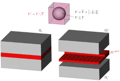
space dimensions, mostly N ∈ {2,3}, and exhibits a periodic microstructure whose length scale is quantified by a small parameter0< ε 1. The modeling of a periodic microstructure relies on the notion of a ‘periodicity cell’ of fixed size, usually denoted

Y. Here, one assumes that the microstructure can be viewed as the disjoint union of translatedε-homothetiesεY of the periodicity cell; see also Figure2.1. To this end, one has to ask thatY has thepaving property,i.e.that one can indeed cover the whole space RN with the disjoint union of translated copies of the periodicity cellY. In symbols, RN =S

j∈N

· (tj +Y)for a family ofRN-vectors{tj : j ∈N}. The microstructure

is then tiled by theε-homothety of this union,i.e.byS

j∈N

· ε(tj+Y). Now, since also

theconstitutive propertiesof the physical system’s microstructure repeat periodically, it suffices to describe them on the periodicity cell by someconstitutive functionA:Y →

Ω

x∈εtj+εY

εtj

tj =:

_x

ε

x

ε ∈tj +Y

x

ε −tj

| {z }

∈Y

Figure 2.1: Illustration of the periodicity cell concept

periodicity celltj+Y containingy, hence one definesA(y) :=A(y−tj). (For such a

microstructure tiling it is convenient to define the functionb·c :RN → _RN _{that maps}

y ∈ _RN _{to the unique translation vectort}

j such thaty ∈ tj +Y. In other words,byc

tells in which translation of the periodicity cell the vectory∈_RN _{lies.) The constitutive}

properties in any material pointxof the microstructure can then be easily determined by evaluatingAε(x) :=A x_ε

(again see Figure2.1). The choice of the periodicity cell depends of course on the specific microstructure under consideration. In the literature, the most commonly used periodicity cell is the unit cube[0,1)N, which I am also going to use in the remainder of this introduction.

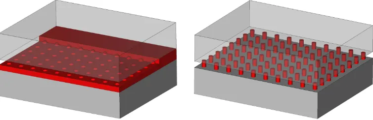
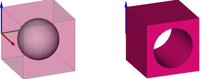
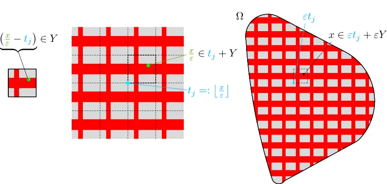
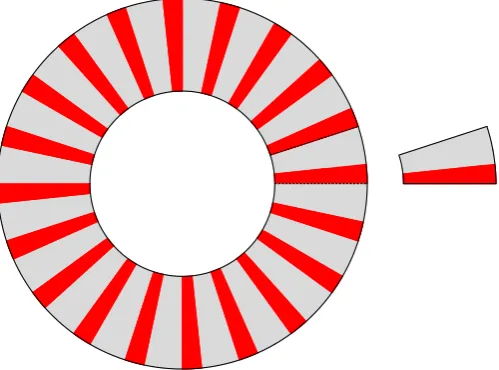
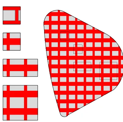
Remark 2.2. There are good reasons for choosing the periodicity cell to be the unit cube, probably the most relevant being simplicity. However, one can easily think of periodic microstructures with periodicity cells different from the cube,e.g. honeycomb-like microstructures whereY becomes a regular hexagon. Hexagonal periodicity cells are most suitable to describe the microstructure in cross-sections of large wire ropes that are made from wires of identical diameter (see Figure2.2, left); here, each wire cross-section can be viewed as the incricle of a regular hexagon, which then make up the wire’s cross-section if arranged like in a honeycomb. Another situation where it appears reasonable to take a periodicity cell different from the unit cube is when the microstructure shows periodically recurring voids – the literature speaks of perforated media – that would touch the periodicity cell’s boundary. However, in some cases on might simply avoid this problem by chosing a suitable periodicity cell, like e.g. in Figure2.2(right); cf. also the recent preprintCioranescu et al.[2011].

ro-Figure 2.2: Hexagonal periodicity cells in cross sections of wire rope

tationsof a periodicity cell; see thefunctionally graded annular diskdepicted in Figure

2.3. Some of these situations may be resolved by changing to an appropriate coordinate

Figure 2.3: A functionally graded annular disk

configurationwith translatory periodic microstructure. However, this reference config-uration would in general be nonatural state,i.e. it would bepre-stressed(see [Ciarlet,

1988, Chapters 2, 3 and 4] for elasticity related terms). There is already some work on prestressed microstructured materials, seeParnell[2007]. Nonetheless, to my opinion there is still much work to do in this field; as concerns the example shown in Figure2.3, I will come back to it in Subsection2.5.2in a more abstract context.

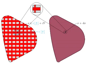
In continuum physics, quantities u(x) ∈ _RK _{that describe the physical state of}

a system in some material point x (it would be better to say in a ‘volume element’

dx around x) are usually related to the constitutive properties inx (or better dx) by partial differential equations. A both physically and mathematically intuitive example is the static heat equation: in this case, the physical system reduces to a (for simplicity solid) body occupying some bounded, smooth domain Ω ⊆ _RN_{, N ∈ {2,3}. The}

constitutive properties, which in general vary within the body Ω, would be given by a thermal conductivity matrixAˆ : Ω → _RN×N_{. Assume furthermore to be given an}

internal heat sourcef : Ω→_R(e.g.heat losses of some technical process) and constant temperature on the body’s boundary (e.g. due to the body being imbedded in a much larger body with far higher thermal conductivity; in appropriate units equal to0). Then, the equation for the equilibrium temperatureu: Ω→Rbecomes

−div Aˆ(x)∇u(x) = f(x) for allx∈Ω, u(x) = 0 for allx∈∂Ω.

Now, if the body had a periodic microstructure with cubic periodicity cellY = [0,1)N, a constitutive functionA : Y → _RN×N _{that tells us how the thermal conductivity}

varies in the periodicity cell, and a microscale parameter0 < ε 1, then the thermal conductivity in a material pointx ∈ Ωis – according to what has been said before –

A x_ε. Thus, the heat equation for the resulting equilibrium temperatureuε : Ω→ R

reads

−div A x_ε∇uε(x)

= f(x) for allx∈Ω

uε = 0 for allx∈∂Ω. (CHP)

Here, it is reasonable to assume that

A(y)is a symmetric matrix for ally ∈Y (A1)

and moreover

    

Ais strongly elliptic,i.e. 1

C|v|

2 _{≤A(y)v·v≤C|v|}2

for allv∈_RN_{, y ∈Y and some constantC >0.}

(A2)

The problem (CHP) is a linear elliptic partial differential equation and if the domainΩ

the thermal conductivityA x_ε

the underlying finite element mesh has to beat leastas fine as the linear size of the periodicity cell,i.e. ε. Hence, the number of mesh nodes is of the same order as the number of periodicity cells inΩ,i.e. of order _ε1N. Plainly

speaking, asεbecomes smaller computation times rise quite rapidly. On the other hand, in applications it is desirable to regard a microstructured material likee.g.the solid body

Ωnot as a complicated geometric arrangement of the microstructure’s constituents, but as one homogeneous material only, maybe at the cost of strong material anisotropy. The reason is that the behavior of single microstructure constituents is often completely out of interest (sometimes they are not even accessible to measurements). It is the macroscopic behavior that counts (see the explanations at the beginning of this section). Hence, if I were an experimental materials scientist, I would ask my laboratory assistant to take a material sample from the solid bodyΩ, lie to him about the microstructure but make him belief that the body’s material is homogeneous and anisotropic, and then simply wait until he comes back with the measured entries of thehomogenizedthermal conductivity matrixAHom ∈RN×N. Having still the same heat sourcef in the bodyΩ

and the same boundary conditions on∂Ω, the resulting temperature distribution in the solid bodyuHom: Ω→Rwould certainly satisfy

−div AHom(x)∇uHom(x)

= f(x) for allx∈Ω uHom(x) = 0 for allx∈∂Ω.

(2.1)

Assuming that the laboratory assistant’s measurements are correct, one has to ask the crucial question: How does this problem relate to the problem (CHP) which resolved the actual microstructure? Is the solutionuεof (CHP) ‘close’ to the homogenized solution

uHomof (2.1) for small enough microscale parametersε? Can one compute the

homog-enized thermal conductivity matrixAHom from the thermal conductivityA _ε·

of the microstructured bodyΩ to avoid costly and time-consuming measurements? In fact, homogenization theory gives positive answers to these questions. More precisely, it es-tablishes convergence of the solutionsuεof the problem with microstructure (CHP) to

the solutionuHomof the homogenized problem (2.1), and also relates the homogenized

constitutive matrixAHom to the original constitutive functionAdefined on the

period-icity cell. Indeed, homogenization theory provides not only one but a whole variety of different methods for this task which allow to study more general mathematical models than the elementary heat equation (CHP). For instance, mathematical models for solid mechanics, fluid mechanics, electromagnetism, biophysics, materials science,. . .

hardware in scientific computing (unless someone invents a standardized graduate stu-dent). Nonetheless, it allows researchers in the field to compare the ‘usability’ of certain methods. For instance, the less problem-specific or homogenization-specific knowledge is required for a certain method, the better; the stronger the topology in which conver-gence to the homogenized solution is shown, the better; and so on... Therefore, all the methods for periodic homogenization I chose to present in this introduction will address the classical homogenization problem (CHP). Moreover, I will point out drawbacks and advantages of certain methods of periodic homogenization when compared to others.

2.2.2 Asymptotic Expansions

The most traditional method in homogenization theory is the so-called method of asymp-totic expansionswhich dates way back to the 1960s. Its basic feature is to postulate that the solutionuε to a problem with periodic microstructure – like (CHP) – is for every

microscale parameterεa series of the form

uε(x) =u0(x) + εu1 x,x_ε

+ ε2u2 x,x_ε

+ . . . (2.2)

with functionsu0 : Ω → Randui : Ω×Y → R,i ∈ N, where the latter are Y

-periodic in their second arguments. Thisansatzreflects the notion thatuε stays close

to some macroscopic partu0 (likewise the solution of the homogenized problem, like

(2.1)) while the microstructure causes small ‘fluctuations’εu1 ·,_ε·

+ε2u2 ·,_ε·

+. . .

around the homogeneous part. With the microstructure beingε-periodic, it is natural to assume that the fluctuations are of the same length scale. As it is natural to assume that these fluctuations vary over the whole domainΩ(e.g. due to external data that varies over the domain, just like the heatingf in (CHP)). Indeed, many mathematical mono-graphs on homogenization theory outline the method of asymptotic expansions (like

Bensoussan et al.[1978];S´anchez-Palencia[1980];Cioranescu and Donato[1999] or

Bakhvalov and Panasenko[1989]), but often little emphasis is given to the motivation of the ansatz (2.2) itself, which though is fundamental to the method. Here, the reader might find [S´anchez-Palencia, 1980, Chapter 5] a very inspiring introduction to the topic. (Generally, in homogenization theory one cannot speak of the method of asymp-totic expansions without giving credit to Evariste Sanchez-Palencia and his numerous important contributions to the topic.) The basic idea of the method of asymptotic expan-sions is now to insert ansatz (2.2) into the equations (CHP) governing the problem with microstructure and to formally apply the differential operator to every component of the series. Sorting the result according to powers of the microscale parameterεand equat-ing the coefficients on both sides of the equation sign leads to a cascade of equations for the functionsu0 andu`,`∈N. Finally, the homogenized problem (2.1) is obtained by

Before applying the method of asymptotic expansions to the classical homogeniza-tion problem (CHP) and deriving the relations between (CHP) and the homogenized problem (2.1) in a ‘personalized’ fashion, I would like to briefly state the method’s principal advantages and drawbacks.

Due to being formal in nature, the method of asymptotic expansion is a simple but universal method to approach various kinds oflinearproblems showing a periodic microstructure. It can basically be applied without any knowledge about the actual so-lution (existence, a priori estimates, compactness, regularity,. . . ) and therefore allows to infer homogenization results more easily and also faster. In addition, the asymptotic expansion method gives the user a good ‘feeling’ about how the single termsu` ·,_ε·

and theirscalingε`,` ∈ _N, contribute to the solution of the microstructured problem

uε. Whereas rigorously justifying an asymptotic expansion of a solution to a problem

with periodic microstructure is usually very hard and problem-specific (in contrast to the universality of the method itself). This is why asymptotic expansions are rarely used to obtain strict convergence of the microstructured problem to the homogenized problem. Moreover, while no knowledge about specific properties of the solution to the microstructured problem is required, the user often needs to have a deep understanding of the problem itself in order to guess the correct form of the asymptotic expansion (e.g.

in case the microstructure shows more than two length scales). Another drawback is that this method usually requires long and cumbersome formal calculations which makes the method quite error-prone. Finally, the asymptotic expansion method is quite unsuitable for problems involving nonlinear differential operators (but not necessarily for nonlin-ear problems in general, seee.g. [S´anchez-Palencia,1980, Chapter 6] orChacha and Sanchez-Palencia[1992]). Nevertheless, although more modern homogenization meth-ods are available for problems with periodic microstructure (see the remainder of the introduction), asymptotic expansion methods are still popular today, both in the math-ematical literature (e.g. Geymonat et al. [2010]; Rohan and Lukeˇs [2010]) and the engineering literature (e.g.Marigo and Pideri[2011]).

In the case of the classical homogenization problem (CHP) with solution uε ∈

W₀1,2(Ω), the asymptotic expansion method with ansatz (2.2) for the solution is as fol-lows. First, the gradient∇uε(x)of the equilibrium temperature in the microstructured

body is formally given through

∇uε(x) =∇u0(x) + ε

∇xu1 x,x_ε

+1_ε∇yu1 x,x_ε

+ε2∇_xu2 x,x_ε

+ 1_ε∇_yu2 x,x_ε

+ . . .

=∇u0(x) +∇yu1 x,x_ε

+

∞

X

`=1

ε`∇<sub>x</sub>u` x,x_ε

+∇_yu`+1 x,x_ε

(2.3)

where∇xu`denotes the gradient ofu`: Ω×Y →Rw.r.t. the first argument and∇yu`

gen-eral not possible to formally apply the divergence operator in (CHP) toA x_ε

∇uε(x),

for the simple reason that the constitutive function,i.e. the thermal conductivity ma-trixA : Y → _RN×N_{, is often not differentiable (but say piecewise constant, if the}

microstructure of the body is made up from two different constituents). In this case I prefer to resort to the weak form of the classical homogenization problem (CHP),i.e.

ˆ

Ω

A x_ε

∇uε(x)· ∇ψ(x) dx=

ˆ

Ω

f(x)ψ(x) dx ∀ψ∈C∞_c (Ω). (2.4)

At this point it is essential to notice the role of ψ ∈ C∞_c (Ω) which has to act as a testfunction for the solutions toallε-problems. In particular, the testfunctionsψhave to be such that they can capture (or ‘sample’) any fine properties of the solutionsuε, most

notably theirε-oscillations. This is why it appears natural to choose testfunctions that also oscillateε-periodically,i.e.

ψ(x) :=ϕ x,x_ε

forϕ∈C∞_c (Ω; C∞_per(Y)),

and therefore

∇ψ(x) =∇xϕ x,x_ε

+1_ε∇yϕ x,x_ε

.

Here,C∞_per(Y)is the space of all smooth functions on the cubic periodicity cell Y = [0,1)N that have identical trace on opposite faces ofY. Then the weak form of (CHP) reads as

ˆ

Ω

A x_ε∇uε(x)· ∇xϕ x,x_ε

+ 1_εA x_ε∇uε(x)· ∇yϕ x,x_ε

dx

= ˆ

Ω

f(x)ϕ x,x_ε

dx ∀ϕ∈C∞_c (Ω; C∞_per(Y)).

Inserting (2.3) and sorting by powers of the microscale parameterεyields

ε0

ˆ

Ω

f(x)ϕ x,x_ε dx

=ε−1

ˆ

Ω

A x_ε

∇u0(x) +∇yu1 x,x_ε

· ∇_yϕ x,x_ε

dx

!

+ε0

ˆ

Ω

A x_ε ∇u0(x) +∇yu1 x,x_ε

· ∇xϕ x,x_ε

+A x_ε ∇xu1 x,x_ε

+∇yu2 x,x_ε

· ∇yϕ x,x_ε

dx

!

+ε1

ˆ

Ω

A x_ε

∇_xu1 x,x_ε

+∇_yu2 x,x_ε

· ∇_xϕ x,x_ε

+A x_ε

∇_xu2 x,x_ε

+∇_yu3 x,x_ε

· ∇_yϕ x,x_ε

dx

!

+. . .

By equating powers of the microscale parameterεon both sides of ‘=’ one obtains the following cascade of equations: For the coefficient ofε−1one has

0 = ˆ

Ω

A x_ε

∇u0(x) +∇yu1 x,x_ε

· ∇_yϕ x,x_ε

dx, (2.6)

for the coefficient ofε0

ˆ

Ω

f(x)ϕ x,x_ε

dx= ˆ

Ω

A x_ε

∇u0(x) +∇yu1 x,x_ε

· ∇_xϕ x,x_ε

+A x_ε

∇_xu1 x,x_ε

+∇_yu2 x,x_ε

· ∇_yϕ x,x_ε

dx, (2.7)

and for the coefficient ofε`,`∈_N,

0 = ˆ

Ω

A x_ε

∇_xu` x,x_ε

+∇_yu`+1 x,x_ε

· ∇_xϕ x,x_ε

+A x_ε

∇_xu`+1 x,x_ε

+∇_yu`+2 x,x_ε

· ∇_yϕ x,x_ε

dx, (2.8)

whereϕ∈C∞_c (Ω; C∞_per(Y)). Now, since the value of the microscale parameterεmay become arbitrarily small one might wonder whether the integrals in (2.6), (2.7) and (2.8) converge. This is indeed the case and can be regarded as thefundamental lemma of periodic homogenization. The version I state here is a simple corollary from [Visintin,

Lemma 2.1. LetΩbe an open and bounded subset of_RN satisfying_1Ω(·+ηk(·))→1Ω

pointwise a.e. in RN _{for every sequence (η}

k)k inL∞(RN) that vanishes uniformly.

Moreover, letY be a bounded and measureable subset of_RN that has the paving prop-erty, and let{tj : j ∈N}be a set ofRN-vectors such thatRN =

S

j∈N

· (tj+Y). Let

f : Ω×Y → _Rbe bounded, continuous in its first variable and in its second variable be extended to the whole_RN byY-periodicity,i.e. f(x, y) := f(x, y− byc). Herein, b·c : RN → _RN _{is the function that maps any y ∈ R}N _{to the unique t}

j such that

y∈tj+Y. Then

(i) we have the identity ˆ

Ω

f x,x_εdx= ˆ

RN _Y 1Ω

εx_ε+εy f εx_ε+εy, y dydx,

(ii) there holds the convergence ˆ

Ω

f x,x_ε dx→ ˆ

Ω Y

f(x, y) dydx asε→0.

Remark2.4. For the common choiceY = [0,1)N or any other periodicity cell of mass

1, the integral mean ffl_Y · · · dy obviously conincides with the unnormalized integral

´

Y · · · dy. However, since all of the thesis’ contents remain valid for other choices of

the periodicity cellY, in particular such of mass different from1, I always explicitely write the integral mean.

Due the lemma’s fundamental role in periodic homogenization I will shortly repeat its proof.

Proof. The basic idea behind the proof is to write the integral´_Ωf x,x_ε dxas an inte-gral over the whole spaceRN, then pave theRN withε-homotheties of the periodicity cellY,i.e. RN ₌ S

j∈N

· ε(tj+Y), and sum up the integrals over the respective tiles

(see also Figure2.1):

ˆ

Ω

f x,x_ε

dx= ˆ

RN1Ω

(x)f x,x_ε

dx=X

j∈N ˆ

ε(tj+Y)

1Ω(x)f x,x_ε

dx

=X

j∈N εN

ˆ

Y 1

Ω(ε(tj+y))f(ε(tj+y), tj+y) dy

=X

j∈N εN

ˆ

Y

1Ω(εtj+εy)f(εtj +εy, y) dy (2.9)

where we performed the change of variablesy := x−tj

ε forx∈ε(tj+Y)and inferred

f(ε(tj +y), tj+y) =f(ε(tj +y), y)from theY-periodicity off in its second

argu-ment. Here it is crucial to notice that for allx∈ε(tj+Y)one has the identity

_x

ε

Moreover, it isεN = _vol1_Y ´_ε(t

j+Y) dy, thus

εN

ˆ

Y 1

Ω(εtj+εy)f(εtj+εy, y) dx

= 1 volY

ˆ

ε(tj+Y)

ˆ

Y 1

Ω(εtj+εy)f(εtj+εy, y) dydx

= ˆ

ε(tj+Y) Y

1Ω ε

_x

ε

+εy

f ε_x

ε

+εy, y

dydx. (2.10)

Equations (2.9) and (2.10) finally yield the first assertion of the lemma. The second assertion follows from the first one and Lebegue’s theorem of dominated convergence. To this end, one realizes that for allx∈_RN _{andy ∈Y}

ε

_x

ε

+εy−x≤ε

_x

ε

−x ε

+ε|y| ≤ε2 sup

˜

y∈Y

|˜y|, (2.11)

hence1Ω ε

_x

ε

+εy f εx_ε+εy, y →_1Ω(x)f(x, y)for a.e. (x, y)∈ _RN _×Y

by the assumptions onΩand the continuity off in its first argument.

Thus, with the help of Lemma2.1, one can for small microscale parameterε ap-proximate (2.6) with

0 = ˆ

Ω Y

A(y) ∇u0(x) +∇yu1(x, y)

· ∇yϕ(x, y) dydx, (2.12)

moreover (2.7) with

ˆ

Ω Y

f(x)ϕ(x, y) dydx= ˆ

Ω Y

A(y) ∇u0(x) +∇yu1(x, y)

· ∇_xϕ(x, y)

+A(y) ∇_xu1(x, y) +∇yu2(x, y)

· ∇_yϕ(x, y) dydx, (2.13)

and (2.8) with (`∈_N)

0 = ˆ

Ω Y

A(y) ∇_xu`(x, y) +∇yu`+1(x, y)

· ∇_xϕ(x, y)

+A(y) ∇_xu`+1(x, y) +∇yu`+2(x, y)

· ∇_yϕ(x, y) dydx, (2.14)

which are to be individudally satisfied byu0 : Ω→ R,u` : Ω×Y → R,`∈N, and

allϕ ∈ C∞_c (Ω; C∞_per(Y)). The final challenge in applying the method of asymptotic expansions is now to infer from the above limiting relations (2.12), (2.13) and (2.14) the equations that the macroscopic partu0 of theansatzforuεsatisfies on the domainΩ.

testfunctionϕ∈C∞_c (Ω; C∞_per(Y))in (2.13) as independent of the second argument,i.e.

with slight abuse of notationϕ(x, y) =ϕ(x)inΩ×Y, then one would obtain

ˆ

Ω

f(x)ϕ(x) dx= ˆ

Ω Y

A(y) ∇u0(x) +∇yu1(x, y)

dy· ∇ϕ(x) dx

∀ϕ∈C∞_c (Ω). (2.15)

This equation is already the weak form of an elliptic partial differential equation foru0

on the domainΩ, and still contains information about the actual microstructure through the constitutive functionA :Y → _RN×N_{. Now, all that remains to do is to determine}

the functionu1; to this end, in (2.12) one takes the testfunction asϕ(x, y) =ρ(x)ψ(y)

forρ∈C∞_c (Ω)andψ∈C_per∞ (Y). By the arbitrariness ofρ∈C∞_c (Ω)this yields in a.e.

x∈Ω

0 =

Y

A(y) ∇u0(x) +∇yu1(x, y)

· ∇_yψ(y) dy ∀ψ∈C∞_per(Y). (2.16)

Upon noticing the linearity of the solution to this equation in∇u0(x), it is convenient

to definewi ∈Wper1,2(Y),i= 1, . . . , N, as the unique solutions of

0 =

Y

A(y) ei+∇ywi(y)

· ∇_yψ(y) dy ∀ψ∈C∞_per(Y) (2.17)

(uniqueness up to an additive constant; existence by the assumptions (A1), (A2) and the Lax-Milgram Lemma). Hence, the functionu1can be uniquely expressed as (again up

to an additive constant)

u1(x, y) =∇u0(x)·

N

X

i=1

wi(y)ei =

  

w1(y)

.. .

wN(y)

 

· ∇u0(x), (2.18)

thus in particular

∇_yu1(x, y) =

h

∇_yw1(y)

· · ·

∇ywN(y) i

∇u0(x).

Inserting this into (2.15) leads to

ˆ

Ω

f(x)ϕ(x) dx

= ˆ

Ω

Y

A(y)I+h∇_yw1(y)

· · ·

∇ywN(y) i

dy

∇u0(x)· ∇ϕ(x) dx

= ˆ

Ω

AHom∇u0(x)· ∇ϕ(x) dx (2.19)

for allϕ∈C∞_c (Ω), where

AHom =

Y

A(y)I+h∇_yw1(y)

· · ·

∇ywN(y) i

Obviously, (2.19) is the weak form of a linear elliptic partial differential equation for the macroscopic partu0of theansatz(2.2). More precisely, it is the weak form of (2.1)

which I motivated earlier in this section by means of physical reasoning. Speaking once more in terms of heat conduction, (2.19) is nothing but the equation for the equilibrium temperature in the bodyΩ, whose microstructure is now so small that it can be regarded as being made from one homogeneous material with constant thermal conductivity ma-trixAHom. Moreover, the equilibrium temperature in the homogenized bodyΩis indeed

the macroscopic partu0in the assumed expansion of the solutionuεto the problem with

microstructure. And thanks to (2.20) one now has a mathematical expression of how to relate the homogenized thermal conductivity matrixAHomto the constitutive properties

of the body with microstructure given throughA _ε·

. Hence, there is no more need to ask a laboratory assistent to determineAHom experimentally. Instead one can simply

computeits entries by means of (2.20) and solving (2.17) (e.g. numerically). In other words, homogenization theory is a way to avoid solvingonecomplicated problem with microstructure (like (CHP)). Yet, it comes at the cost of solvingtwosimpler problems. One to compute the homogenized constitutive propertiesAHom (by (2.17) and (2.20))

which are inferred exclusively from the microstructure,i.e. the periodicity cell Y and how the constitutive properties vary over the periodicity cell byA:Y →_RN×N_{. And}

another one to determine the solutionuHom to the homogenized problem,i.e. (2.1) or

equivalently (2.19). Plainly speaking, the homogenization process leads – as expected – to aseparation of scales. Due to the importance of the above homogenization results to the upcoming parts of the introduction and homogenization theory in general, at the cost of some redundancy I will state it once again as a self-contained definition.

Definition 2.2. LetY = [0,1)N be theN-dimensional unit cube and the constitutive functionA : Y → _RN×N _{be such that it satisfies the assumptions (A1) and (A2).}

Moreover, letwi ∈Wper1,2(Y),i= 1, . . . , N be the (up to an additive constant) unique

solutions of

0 =

Y

A(y) ei+∇ywi(y)

· ∇yψ(y) dy ∀ψ∈C∞per(Y).

Then, thehomogenized constitutive matrixAHom ∈RN×N is defined through

AHom =

Y

A(y)I+h∇_yw1(y)

· · ·

∇ywN(y) i

dy.

Still, although one now has a way to calculate the homogenized thermal conductivity matrix AHom, it is a priori not clear whether it also has the natural properties of a

conductivity matrix. Or, more mathematically speaking, whetherAHomis ‘nice enough’

to ensure the existence of a solution to the homogenized problem (2.1). The answer is found in the following statement.

Proposition 2.3. LetY, A : Y → _RN×N_{, A}

Hom ∈ RN×N andwi ∈ W1per,2(Y) be

(i) AHomis symmetric and strongly elliptic,i.e.

1 C|v|

2_≤A

Homv·v≤C|v|2

for some constantC >0.

(ii) AHomcan be written as

AHom,ij = Y

A(y) ej+∇ywj(y)

· ei+∇ywi(y)

dy,

i, j ∈ {1, . . . , N}.

This is again one of the fundamental results of periodic homogenization, which is why I chose to provide a proof (as found in e.g [Bensoussan et al., 1978, Chapter 1, Remark 2.6], [S´anchez-Palencia, 1980, Chapter 5, Section 3] or [Cioranescu and Donato,1999, Proposition 6.9]).

Proof. Obviously, the second assertion and the symmetry ofAby (A1) imply the sym-metry ofAHom. To prove the second statement, one first writes fori, j∈ {1, . . . , N}

Y

A(y) ej+∇ywj(y)

· ei+∇ywi(y)

dy

=

Y

A(y)ej·eidy

+

Y

A(y)ej· ∇ywi(y) dy+

ˆ

Y

A(y)∇_ywj(y)·eidy

+

Y

A(y)∇_ywj(y)· ∇ywi(y) dy.

However, testing the equation (2.17) definingwj withwiyields

0 =

Y

A(y)ej· ∇ywi(y) dy+

ˆ

Y

A(y)∇wj(y)· ∇ywi(y) dy,

thus

Y

A(y) ej+∇ywj(y)

· ei+∇ywi(y)

dy

=

Y

A(y)ej·eidy+

ˆ

Y

A(y)∇ywj(y)·eidy

=

Y

A(y)I+h∇_yw1(y)

· · ·

∇ywN(y) i

dy ej

·ei

=AHom,ij

and the second assertion follows. It remains to prove the ellipticity of AHom. Since

AHomv·v >0for allv ∈RN \ {0}. For suchvobserve that by the second statement

of the proposition

AHomv·v=

N

X

i,j=1

viAHom,ijvj

=

Y

A(y)

 

N

X

j=1

vj ej +∇ywj(y)

 ·

N

X

i=1

vi ei+∇ywi(y)

!

dy.

An easy calculation shows thatPN

i=1vi ei+∇ywi

is nothing but the gradient of the functionζv ∈W1,2(Y), ζv(y) :=PN_i=1vi yi+wi(y)

, and by the ellipticity (A2) of

Aone infers

AHomv·v≥

1

C _Y |∇yζv(y)|

2_dy.

If the right hand side were zero, then ζv would result as a constant function, hence

ζv ∈ W1per,2(Y). SinceW1per,2(Y)is obviously a vector space, one would further obtain

Y 3y7→v·y=ζv−

PN

i=1viwi ∈Wper1,2(Y). This however is only possible ifv= 0,

which contradicts the assumptionv∈_RN _{\ {0}. ThusA}

Homis positive definit and the

proof is finished.

With the ellipticity ofAHomat hand, the Lax-Milgram Lemma immediately yields

the existence of a unique solution to the homogenized equation (2.1), more precisely to its weak form (2.19). Thus, the problem defining the macroscopic partu0 of theansatz

(2.2),i.e.the equilibrium temperatureuHomin the homogenized bodyΩ, is well-posed.

Remark 2.5. I would like to advice the reader that homogenization does not always conserve the mathematical ‘nature’ of a problem with microstructure, although this is the case for the classical homogenization problem (CHP) and its homogenized counter-part (2.1). In fact, the homogenization process may lead to ‘strange phenomena’ like

e.g.in [Cioranescu et al.,2011, Theorem 5.13], where the authors observe entirely new boundary conditions in the homogenized equations caused by periodically recurring microscopic quantitiesinsidethe microstructured domain.

Although the derivation of the homogenized equations (2.1) and the homogenized constitutive properties (see Definition2.2) has been completely formal, in the case of the classical homogenization problem (CHP) one can indeed justify theansatz (2.2). For this one might turn to e.g. [Bensoussan et al., 1978, Chapter 1, Section 2.4] or [Cioranescu and Donato,1999, Section 7.2]. However, the justification heavily relies on regularity theory for solutions of elliptic partial differential equations and therefore requires additional smoothness assumptions on the domain and the data. In order to obtain strict convergence of the solutionsuεfor the problem with microstructure (CHP)

to the solutionuHom of the homogenized problem (2.1), other methods for periodic

Before turning to other methods in the theory of periodic homogenization, I would like to state a critical remark regarding the presence, or better, the absence of asymp-totic expansions in lectures on periodic homogenization for students of mathematics. In fact, many lecture notes or books on periodic homogenization I have come across in the past four and a half years hardly teach the method of asymptotic expansions but merely include it for seemingly historic reasons. An argument which is often heard among mathematicians is that its formal nature would make it an engineer’s method rather than a mathematician’s method and that homogenization theory is about proving convergence to a homogenization limit. As concerns proving convergence of a problem with microstructure to a homogenization limit, there are indeed more suitable methods available than asymptotic expansions. However, I tend do disagree with the opinion that homogenization theory is about proving convergence – it’s about deriving the ho-mogenization limit, whereas proving convergence is about showing that the obtained homogenization limit is correct. In fact, the steps leading to the identification of the homogenization limit for the classical homogenization problem exposed in this section areself-contained and cover little more than 5 pages. Whereas proving convergence in a self-contained fashion would require considerably more efforts (even when using a very generous definition of the term ‘self-contained’). While there is definitely a need to prove convergence, to my opinion it is nonetheless very useful to employ a fast and simple method beforehand to derive the homogenization limit, no matter how formal or ‘quick and dirty’ the method may be. After all, this is why the asymptotic expansion method is still popular today, even in the mathematical literature (see the examples I gave previously). Another advantage of asymptotic expansions in periodic homogenization is that it isconstructive and allows for an explicit calculation of the homogenization limit rather than producing abstract existence results (e.g. from com-pactness arguments). To conclude, I would strongly advocate a more prominent role of the asymptotic expansion method in courses on periodic homogenization for students of mathematics, as well as examples of its use in contemporary research.

2.2.3 Γ-convergence

for the minimizer of a quadratic functional: by definition

uε∈W01,2(Ω)solves (_ˆ CHP) ⇔

Ω

A x_ε∇uε(x)· ∇ψ(x) dx=

ˆ

Ω

f(x)ψ(x) dx ∀ψ∈C∞_c (Ω)

and by density for allψ∈W1₀,2(Ω). But this is indeed the Euler-Lagrange equation for the unique minimizeruεof the functional

E_ε: W1₀,2(Ω)→_R,

Eε(v) := 1₂

ˆ

Ω

A x_ε∇v(x)· ∇v(x) dx− ˆ

Ω

f(x)v(x) dx (2.21)

(uniqueness by the strong ellipticity (A1) of the constitutive function A). Physically speaking, Eε can be interpreted as the dissipation potential (see e.g. [Lemaitre and

Chaboche,1990, Chapter 2.5]) for the heat conduction in the microstructured bodyΩ, and the minimizer of the dissipation potential is actually the body’s equilibrium tem-peratureuε. Hence, as Marcellini realized the classical homogenization problem (CHP)

can for varying values of the microscale paremterεbe viewed as sequence of function-als(E_ε)ε indexed byε. More specifically, as a sequence of minimization problemsor

variational problems. By physical intuition, as well as bye.g.the method of asymptotic expansions one already knows that there is a homogeneous approximation (2.1) for the classical homogenization problem (CHP) and that the corresponding solutionsuε–i.e.

the minimizers ofEε– converge in a certain sense to the solutionuHomof the

homoge-nized problem (2.1). However, the homogenized equation (2.1) is again nothing but the Euler-Lagrange equation of thehomogenized functional

E_Hom : W1₀,2(Ω)→_R,

EHom(v) := 1₂

ˆ

Ω

AHom∇v(x)· ∇v(x) dx−

ˆ

Ω

f(x)v(x) dx (2.22)

whereAHom is the homogenized constitutive matrix as given in Definition2.2. In

par-ticular,uHom can therefore be viewed as the unique minimizer ofEHom (uniqueness by

the ellipticity ofAHom, see Proposition2.3). Consequently, given convergence of the

solutionsuεto (CHP) to the solution ofuHom of the homogenized problem (2.1), one

can express this like

arg min

v∈W₀1,2(Ω)

Eε(v) =uε −−−→

ε→0 uHom = arg min

v∈W₀1,2(Ω)

EHom(v) (2.23)

Now, one may ask whether there is a notion of convergence for sequences of function-als like(Eε)εto some limit functionalEHomthat ensures convergence of the minimizers

(uε)εto a minimizer of the limit functional, here denoteduHom. Indeed, this is whatΓ

coercivity and compactness assumptions on the functionals and the underlying vector space every cluster point of the corresponding sequence of minimizers is a minimizer of theΓ-limit functional. Moreover, the associated sequence of minima also converges to the minimum of theΓ-limit. (The term ‘energy functional’ is commonly used in the context ofΓ-convergence. In applications ofΓ-convergence to continuum physics, the functionals encountered often quantify the energy ‘stored’ in a certain configuration of the underlying physical system. Comparee.g. Γ-convergence approaches to problems of elasticity, like those inFriesecke et al.[2002] orLe Dret and Raoult [1995], where suitable functionals capture the stored elastic energy of the underlying system.) This is why Paolo Marcellini inMarcellini [1978] employed methods closely related toΓ -convergence (although the term ‘Γ-convergence’ is never stated in that article). Yet, he did not only derive the homogenized equations for the classicallinearhomogenization problem, but for a far wider class of nonlinear homogenization problems. This was due to the major advantage thatΓ-convergence requires no or only minor assumptions on the particular form of the functionalsEε. In principle, any homogenization problem

that can be viewed as a sequence of minimization problems,i.e. as a sequence func-tionals index by the microscale parameter ε, can be approached with Γ-convergence methods. Most notably, linearity or nonlinearity or even the existence of associated Euler-Lagrange equations is of no importance toΓ-convergence. The other main inno-vation in Marcellini’s contribution was the representation of the homogenized problem. Previous approaches, likee.g. the asymptotic expansion method I exposed earlier, al-ways described both the homogenization limit of the classical homogenization problem (CHP) and the homogenized constitutive matrixAHomby means of – as I have to admit

– complicated and rather unintuitive partial differential equations (see Definition2.2and Proposition2.3). Instead, theΓ-convergence approach allows for a representation of the homogenized problem completely in terms of minimization problems. In fact, not only the homogenized equation (2.1) can be replaced by finding a minimizer to the functional

EHom as defined above, but also the equations leading to the homogenized constitutive

matrixAHom. A close look to the definition of the auxiliary functionsw1, . . . , wN from

whichAHomis computed (see Definition2.2) and the very same arguments that revealed

(CHP) and (2.1) to be Euler-Lagrange equations shows that

0 =

Y

A(y) ei+∇ywi(y)

· ∇_yψ(y) dy ∀ψ∈C∞_per(Y) ⇔

wi = arg min v∈Wper1,2(Y)

Y

1

2A(y) ei+∇yv(y)

· ei+∇yv(y)

dy

for alli= 1, . . . , N. More generally, for arbitraryF ∈_RN _withw

F :=PNi=1Fiwi∈

Wper1,2(Y)one identifies the following minimization problem

0 =

Y

A(y) F +∇ywF(y)

· ∇yψ(y) dy ∀ψ∈C∞per(Y)⇔

wF = arg min v∈W1per,2(Y)

Y

1

2A(y) F+∇yv(y)

· F +∇_yv(y)

dy