Model-driven Autotuning of Sparse
Matrix-Vector Multiply on GPUs
Jee W. Choi
Georgia Institute of Technology, School of Electrical and Computer Engineering
Atlanta, Georgia, USA [email protected]
Amik Singh
Indian Institute of Technology Roorkee, Department of Electronics and Computer
Engineering, Roorkee, India [email protected]
Richard W. Vuduc
Georgia Institute of Technology, Computational Science and EngineeringDivision Atlanta, Georgia, USA
Abstract
We present a performance model-driven framework for automated performance tuning (autotuning) of sparse matrix-vector multi-ply (SpMV) on systems accelerated by graphics processing units (GPU). Our study consists of two parts.
First, we describe several carefully hand-tuned SpMV imple-mentations for GPUs, identifying key GPU-specific performance limitations, enhancements, and tuning opportunities. These im-plementations, which include variants on classical blocked com-pressed sparse row (BCSR) and blocked ELLPACK (BELLPACK) storage formats, match or exceed state-of-the-art implementations. For instance, our best BELLPACK implementation achieves up to 29.0 Gflop/s in single-precision and 15.7 Gflop/s in double-precision on the NVIDIA T10P multiprocessor (C1060), enhanc-ing prior state-of-the-art unblocked implementations (Bell and Garland, 2009) by up to 1.8×and 1.5×for single- and double-precision respectively.
However, achieving this level of performance requires input matrix-dependent parameter tuning. Thus, in the second part of this study, we develop a performance model that can guide tuning. Like prior autotuning models for CPUs (e.g., Im, Yelick, and Vuduc, 2004), this model requires offline measurements and run-time es-timation, but more directly models the structure of multithreaded vector processors like GPUs. We show that our model can iden-tify the implementations that achieve within 15% of those found through exhaustive search.
Categories and Subject Descriptors C.4 [Computer Systems Or-ganization]: Performance of Systems—Modeling Techniques
General Terms Algorithms, Performance
Keywords GPU, sparse matrix-vector multiplication, performance modeling
1.
Introduction
We consider thesparse matrix-vector multiply(SpMV) operation for platforms based on graphics processing units (GPUs). Our
moti-Permission to make digital or hard copies of all or part of this work for personal or classroom use is granted without fee provided that copies are not made or distributed for profit or commercial advantage and that copies bear this notice and the full citation on the first page. To copy otherwise, to republish, to post on servers or to redistribute to lists, requires prior specific permission and/or a fee.
PPoPP’10, January 9–14, 2010, Bangalore, India.
Copyright c2010 ACM 978-1-60558-708-0/10/01. . . $10.00
vation comes from two well-known facts: (1) To first order, stream-ing the matrix should dominate SpMV performance, and so SpMV is largely memory bandwidth-bound; and (2) current and emerg-ing GPUs are bandwidth-rich computemerg-ing platforms, today offer-ing peak bandwidths an order of magnitude higher than those of conventional multicore platforms based on general-purpose CPUs. Thus, SpMV and GPUs should be a perfect match.
The challenge is that SpMV is anirregularcomputation that, in addition to streaming, requires many indirect and irregular memory accesses. This memory behavior contrasts starkly to that of dense linear algebra kernels, such as LU, QR and Cholesky factorizations, for which highly efficient implementations exist that achieve hun-dreds of Gflop/s on a single GPU [17]. An SpMV incurs the over-head of moving integer indices (meta-data) that track which non-zeros are stored, and furthermore performs many indirect loads.
Indeed, from a productivity perspective, the dense and sparse cases for matrix-vector multiply differ markedly. Without prior knowledge of NVIDIA GPUs and using only the information pro-vided in the CUDA programming guide [1], we wrote a dense matrix-vector multiplication kernel that achieves 92% of the band-width measured using thebandwidthTestprogram provided with the CUDA SDK.1Achieving even half the performance for SpMV
required significantly more effort, including designing a suitable data structure as well as careful tuning. Our SpMV implementation contains roughly twice the number of lines of CUDA code as the dense counterpart.
Findings and contributions. This paper makes several contribu-tions.
First, we implement the classical blocked version of CSR (BCSR) and study the effects of common GPU optimizations on the kernel. Tuning BCSR for GPUs differs markedly from an equiv-alent CPU implementation. From this experience, we design and implement a new sparse matrix compression format, called BELL-PACK, tuned for GPUs. This format extends ELLPACK/ITPACK format [14] with (a) explicit storage of dense blocks to compress the data structure, and (b) row permutation to avoid unevenly dis-tributed workloads. The absolute performance achieved, up to 29.0 Gflop/s in single-precision and 15.7 Gflop/s in double-precision on a single NVIDIA T10P multiprocessor-based GPU, enables improvements over the best unblocked state-of-the-art implemen-tation by up to 1.8×and 1.5× for single and double-precision computations respectively [3].
However, BELLPACK requires careful tuning. Thus, we pro-pose a novel and accurate performance model-driven framework
1At the time, up to over twice the performance of thecublasSgemvkernel
for autotuning SpMV, based on an abstract execution model of a GPU. This framework, based on the paradigm of offline bench-marking combined with a model instantiated at run-time [11], se-lects the correct tuning parameters with a median error relative to exhaustive search of less than 15%.
Limitations. Our study is encouraging but not without limita-tions. First, the improvements due to BELLPACK apply only to matrices that have small dense block sub-structures; however, this class is still fairly broad as it includes matrices arising in applica-tions based on the finite-element method. Also, using BELLPACK involves re-packing the data from its original form, such as CSR, which incurs a run-time cost. However, this cost is inherent in any autotuning scheme that considers transformations of the data struc-ture [11, 18].
Our execution model of the GPU is our first attempt, and does not directly model some costs, such as thread block scheduling costs, which we believe to be small. Also, although the autotuning framework can be extended to other GPU-like multithreaded SIMD architectures, we test it in this paper on only two NVIDIA Tesla series GPUs on two different kernels. Extending this framework to other architectures may require some modifications or additions to the model. Nevertheless, we believe that, by validating on an irregular computation, we complement the most sophisticated GPU models developed to date [10].
2.
Related Research
The literature on SpMV optimization and tuning is extensive. We review the most relevant work here, and refer the interested reader to other surveys [7, 11, 19].
This paper follows in the spirit of the paper by Williams, et al., which evaluates SpMV for several multicore platforms, includ-ing the Sony-Toshiba-IBM Cell/Broadband Engine (STI Cell/B.E.) but excluding GPUs [21]. Bell and Garland consider several meth-ods, including a variation of ELLPACK that differs from ours [3]. They split the storage between an ELLPACK and coordinate for-mat to reduce its footprint, a novel variant of other previously pro-posed splitting methods [9, 13, 20]. At the same time, Baskaran and Bordawekar proposed a general compile- and run-time infrastruc-ture, evaluated for SpMV [2]. They seem to achieve performance roughly comparable to Bell and Garland on similar hardware.
Bolz, et al., published the first paper in 2003 on GPU-based SpMV (plus higher-level multigrid and conjugate gradient solvers) of which we are aware [4]. They achieved a high fraction (∼ 1/3) of GPU peak for structured grids. Sengupta, et al., developed more generic approaches using parallel prefix/scan primitives [16], though this implementation did not at the time outperform CPU-based codes [8, 16]. Christen and Schenk accelerate the dense part of a sparse direct solver, whereas SpMV-centric studies implicitly target iterative solvers [5].
The row permutation employed by our proposed BELLPACK format is directly inspired by early work on vectorized SpMV, which is especially relevant to GPUs. This prior work includes jagged diagonal or clever row/column permutations combined with traditional formats [6, 12, 13].
3.
NVIDIA CUDA and Experimental Setup
NVIDIA’s CUDA is a programming model designed for the data-parallel processing capabilities of NVIDIA GPUs. A CUDA pro-gram consists of ahost programthat runs on the CPU host, and a kernel programthat executes on the GPU itself. The host program typically sets up the data and transfers it to and from the GPU, while the kernel program processes that data.The CUDA model has two key components. The first is the concept of fine-grainedthreads, which are grouped into
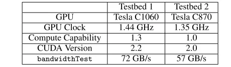
coarser-Testbed 1 Testbed 2
GPU Tesla C1060 Tesla C870
GPU Clock 1.44 GHz 1.35 GHz
Compute Capability 1.3 1.0
CUDA Version 2.2 2.0
bandwidthTest 72 GB/s 57 GB/s
Table 1. NVIDIA GPU testbeds used in our study.
grainedthread blocks. Threads within a block share a local-store and may synchronize via barriers. There is no such synchronization mechanism for threads in different thread blocks.
The second component is the memory hierarchy. The main memory in a GPU is a high-bandwidth DRAM in a shared ad-dress space. There is also a low-latency per-thread-block on-chip memory called the shared memory and a per-thread private local memory in the form of registers. There are also two types of read-only memory calledconstant memory and texture memory, also uniformly addressable by all threads.
The CUDA Programming Guide offers several tips for maxi-mizing performance [1]. (1) Maximize the bandwidth from global memory using coalesced loads. (2) The latency from the on-chip shared memory is comparable to that of the register file. Therefore, shared memory should be used to store data that is shared amongst the threads and/or reused frequently. (3) Resource usage—the num-ber of threads, amount of shared memory, and the numnum-ber of reg-isters used by a single thread block—determines multiprocessor utilization, and kernels must carefully balance usage of these re-sources. Other “folk” methods include loop unrolling, interleaving memory accesses and processing to hide memory latencies. Volkov and Demmel offer additional techniques, and argue that a suitable machine abstraction for GPUs is that of a multithreaded local-store vector architecture [17].
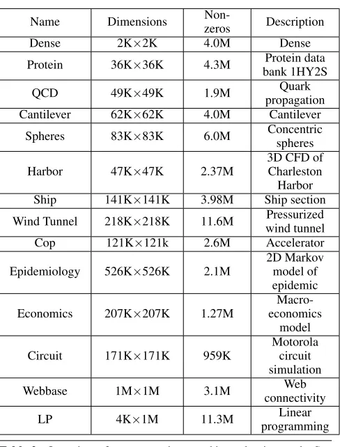
Experiments. All experiments in this paper were run on either or both of the two systems listed in Table 1, and using the sparse matrix benchmark suites in Table 2, which are used in prior work by others [3, 21].
4.
Hand-optimizing Baseline BCSR
This section describes a basic blocked compressed sparse row (BCSR) implementation that extends the state-of-the-art GPU CSR implementation [3]. From this basic implementation, we identify key factors that prevent the algorithm from achieving better perfor-mance and hand-optimize the kernel accordingly.
4.1 CSR and BCSR
The conventional CSR format stores anm×nsparse matrix having
knon-zero elements using three one-dimensional arrays: the arrays valandcol ind, each of sizek, to store the non-zeros values and column indices, respectively; and an arrayrow ptrof sizem+ 1
to store pointers to the first element of each row in thevaland col indarrays. In the implementation by Bell and Garland, a warp of threads is assigned to each row of the matrix, with each thread performing a multiply-accumulate on the non-zeros in the row in an interleaved manner. After all non-zeros have been processed and stored in the shared memory (local-store), the warp executes a parallel reduction to produce the final value.
In the blocked variant of CSR, BCSR, we storer×c dense subblocks of non-zeros rather than storing each non-zero individ-ually [15], as illustrated in Figure 1. Depending on the matrix, we can in principle reduce the column index storage by up to roughly
1
Name Dimensions
Non-zeros Description
Dense 2K×2K 4.0M Dense
Protein 36K×36K 4.3M Protein data
bank 1HY2S
QCD 49K×49K 1.9M Quark
propagation
Cantilever 62K×62K 4.0M Cantilever
Spheres 83K×83K 6.0M Concentric
spheres
Harbor 47K×47K 2.37M
3D CFD of Charleston Harbor
Ship 141K×141K 3.98M Ship section
Wind Tunnel 218K×218K 11.6M Pressurized wind tunnel
Cop 121K×121k 2.6M Accelerator
Epidemiology 526K×526K 2.1M
2D Markov model of epidemic
Economics 207K×207K 1.27M
Macro-economics
model
Circuit 171K×171K 959K
Motorola circuit simulation
Webbase 1M×1M 3.1M Web
connectivity
LP 4K×1M 11.3M Linear
programming
Table 2. Overview of sparse matrices used in evaluation study. See also Williams, et al. [21].
X X X X
X X X X X
X X
X X X
X X
X X 8
8 0 3 4 5 7
X X X 0 X 0 0 X X X X X X X 0 0 X X 0 X X 0 0 X 0 X 0 X
0 2 6 2 0 2 4
B0 B1 B2
B3
B4
B5 B6
row_bptr
bval
col_bind
B0 B1 B2 B3 B4 B5 B6
2 2
Figure 1. The BCSR compression format.
Given a matrix in CSR, we implement BCSR by statically dividing the matrix into(m
r)×( n
c)sub-blocks of sizer×ceach, with explicit padding of zeros as needed.
Our initial BCSR implementation begins with a straightforward adaptation of the CSR baseline of Bell and Garland [3]. In par-ticular, we store elements of eachr×cblock contiguously and assign each thread to anr×cblock, combining the results within a
block row via parallel reduction. The pseudocode for SpMV when
r=c= 2appears in Algorithm 1.
Algorithm 1: 2×2 BCSR kernel to computey←y+A·x
Input:m×nmatrixA, stored in BCSR(r×c) format as (bval,col bind,row bptr);
vectorsxasx[1. . . n],yasy[1. . . m] Output: Modifiesy
LetTB= thread block size (1-D) Lettid= local thread ID Initializesdata[TB][2]
for each block row,Ido
1
row start=row bptr[I]
2
row end=row bptr[I+ 1]
3
fork=row bptr[I];k<row bptr[I+ 1];k=k+TBdo
4
for each threaddo
5
j0=col bind[k+tid]
6
float4 tmp=bval[k+tid]
7
sdata[tid][0] +=tmp.x×x[j0] +tmp.y×
8
x[j0+1]
sdata[tid][1] +=tmp.z×x[j0] +tmp.w×
9
x[j0+1]
parallel reduction in shared memory tosdata[0][0]
10
parallel reduction in shared memory tosdata[0][1]
11
Y[I×2] +=sdata[0][0]
12
Y[I×2+1] +=sdata[0][1]
13
The performance of this baseline implementation is poor, owing largely to uncoalesced memory accesses. We address this issue through the transformations described below.
4.2 Short Vector Packing
Because each thread is assigned to a particularr×cblock and each block is stored contiguously asr×cfloats, threads within a warp will access data in a non-contiguous manner, leading to a deterioration in performance.
We can partially alleviate this problem by first loading data in larger granularities. In particular, we exploit CUDA’s built-in short-vector data types,float2,float3, andfloat4, which correspond to 32-, 64-, and 128-bit vectors. Whenr×cis small, e.g.,2×2,
3×1, or1×4, the entire block will fit into a single short vector, so that threads within a warp issue contiguous short-vector loads, thereby reducing the instruction count and improving bandwidth utilization.
If anr×cblock requires more than 1 short vector, we will still have non-contiguous loads if we store the multiple short vectors contiguously (addressed below). For1×3,3×1, and3×3blocks, we find empirically that it is generally better to usefloat4storage with padded zeros, sincefloat4is automatically aligned [1].
4.3 Row Alignment
0 0.1 0.2 0.3 0.4 0.5 0.6 0.7 0 5 10 15 20 25 Dense Protein QCD Cantilever Spher es Harbor Ship Wind T unnel Accelerator Epidemiology Economics Circuit
Web LP
Fraction of Estimated Empirical Peak
Gflop/s
BCSR + Short vec. pack +Align & Interleave CSR NVIDIA (best)
Figure 2. Single-precision performance (Gflop/s) of the best BCSR kernels for each test matrix. The estimated empirical peak (secondary y-axis on right) assumes an ideal 2 flops per 4 bytes streamed at the empirical peak bandwidth of 72 GB/s. This band-width is reported by the CUDA SDKbandwidthTestbenchmark.
4.4 Interleaved Memory Accesses
When multiple short-vector words are required to store anr×c
block, we can avoid non-contiguous short vector access within a warp by interleaving words from consecutive blocks.
4.5 Experimental Results
We compare the BCSR implementations to the NVIDIA imple-mentations [3] on the NVIDIA C1060 (T10P-based) platform in Figure 2. The block size is tuned exhaustively up to4×4, report-ing the best case. Not surprisreport-ingly, the final BCSR implementation outperforms the baseline CSR implementation for matrices with natural dense block substructure—Protein through Accelerator, as these matrices come predominantly from simulations based on the finite-element method.
However, the NVIDIA’s best implementations using other for-mats (e.g., the hybrid ELLPACK+coordinate (COO) scheme) still outperform our best BCSR code in several cases. Our best BCSR rarely exceeds 50% of the estimated peak for single-precision dense matrix-vector multiply. Thus, even if the application is bandwidth-limited like SpMV, simply reducing the data size is inadequate— special optimizations are also necessary to achieve still higher per-formances on GPUs.
5.
Blocked ELLPACK
Although the BCSR improves over CSR, it still falls far short of NVIDIA’s best implementation (Figure 2). The major bottleneck comes from the parallel reduction step, whose performance is sen-sitive to the number of blocks available in a particular block row, which can be small (e.g., less than 20). Given the similarity be-tween current GPUs and vector architectures [17], we might in-stead prefer a vector-friendly format such as the classical ELL-PACK/ITPACK format [14]. Indeed, the best NVIDIA format is often (but not always) their hybrid ELLPACK+COO scheme [3]. Therefore, we also consider a blocked ELLPACK (BELLPACK) format that combines the advantages of the dense subblock storage of BCSR and the vector-friendly ELLPACK format.
In classical ELLPACK, we store anm×nmatrix using twom× L arrays, for the values and column indices, respectively, where
X X X X X X X X X X X X X X X X X X X X X R R Λ0 Λ1 ... R Λi
B0,0 B0,1
B1,0 B1,1
B1,1
B1,1[0] B1,1[1]
B1,1[2] B1,1[3]
B0,0[0] B1,0[0]
B0,0[1] B1,0[1]
B0,0[2] B1,0[2]
B1,0[3] B0,0[3]
R
B1,1[0] B0,1[0]
B1,1[1] B0,1[1]
B1,1[2] B0,1[2]
B1,1[3] B0,1[3]
K0
r
c
Ki× r × c
thread 0 thread 1 Processed by thread block i
... Ki K0 K1 # r × c blocks per TB
... column index
CI0
CI1
CIi
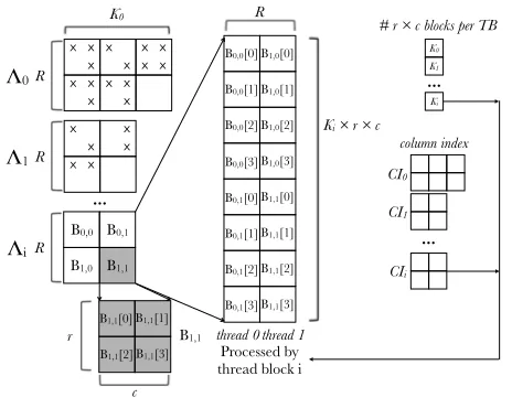
Figure 4. Storage of block rows in BELLPACK
Lis the maximum number of non-zeros in any row. That is, an ELLPACK matrix is stored using twom×LarraysVandJsuch that V[i,k] is the matrix entryA(i,J[i,k]). Rows with fewer thanL non-zeros are padded with non-zeros, which results in unnecessary storage and flops (work). However, this format suits GPUs well because it is easy to (a) vectorize SpMV within a columnV[·,k], given indirect addressing support; (b) align the matrix data for efficient global memory transfers; and (c) do 1-D block row-based partitioning. Storingr ×c dense subblocks is a straightforward adaptation, helping to reduce column index storage as with BCSR. However, ELLPACK peforms poorly when the variance in the number of non-zeros per row is high, thereby necessitating excessive zero-padding.
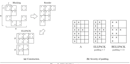
5.1 Our Blocked ELLPACK Implementation
Conceptually, we construct a BELLPACK matrix from am×n
input matrixAas sketched in Figure 3(a) and described as follows.
Basic storage scheme. First, we logically reorganize A into a new matrix, A0, stored using r×c dense subblocks. This step helps reduce column index storage, as with BCSR. We then sort the block-rows in descending order of number of blocks per row, resulting in a new matrixA00. The sort step is identical to what is done for the so-called jagged diagonal format [15], and corresponds to applying a row permutation,Pr, toA0, i.e.,A00=Pr·A0. Finally, we partition the rows ofA00into m
R non-overlapping submatrices, each of sizeR× n
c. We store each submatrix in ELLPACK or r×cblocked ELLPACK format. This partitioning step helps to reduce the padding that would otherwise result in matrices with a high variance in the number of non-zeros per row, as suggested in Figure 3(b).
Block row-partition layout. To encourage coalescing, we store eachR×n
c block row,Λi, as illustrated in Figure 4. In particular, the values ofΛiare laid out in a 2-D row-major array (middle of Figure 4). Each column contains all of the data to-be-accessed by a particular thread, laid outr×cblock-by-block. The unit-stride dimension is across rows of this array, to ensure coalescing. This array is aligned and padded as necessary. A parallel structure is used to store the block column indices (right side of Figure 4).
X X X
X X
X X X X
X X X X X
X X X
X X
X X
X X
X X
X X X X X X
X X X
X X X
X X X X
X
Reorder Blocking
X X
X X
X X X X X X
X X X
X X X
X X X X
X
ELLPACK
r
c
R
R
m
n
(a)Construction.
A
ELLPACK
padding = 7
BELLPACK
padding = 13
X X
X
X X X
X X
X X
X
X X
X
X X X
X X
X X
X
X X
X
X X X
X X
X X
X
(b)Severity of padding. Figure 3. BELLPACK format.
Our implementation uses the texture cache to load the values of vectorx, as done by Bell and Garland [3]. We also tried explicit blocking and use of the local-store shared memory but found the texture cache approach to be both simpler and more effective em-pirically.
Algorithm 2: 2×2 BELLPACK kernel to computey ←y+ A·x
Input: array of arraysAd valuesfor values andAd indexfor indices, arrayAd numBlocksfor block sizes, vectorx asx[1. . . n], and blocking sizesrandc
Output: Modifiesy Letbid= block ID Lettid= local thread ID LetTB= thread block size (1-D) if tid== 0then
1
numBlocks=Ad numBlocks[bid]
2
A values=Ad values[bid]
3
A index=Ad index[bid]
4
fori= 0to numBlocks do
5
col Index=A index[TB×i+tid]×c
6
xval=x[col Index]
7
rs 1+=A values[TB×4×i+tid]×xval
8
rs 2+=A values[TB×4×i+TB×2+tid]×xval
9
xval=X[col Index++]
10
rs 1+=A values[TB×4×i+TB×1+tid]×xval
11
rs 2+=A values[TB×4×i+TB×3+tid]×xval
12
y[TB×bid×2+tid×2] =rs 1
13
y[TB×bid×2+tid×2 +1] =rs 2
14
5.2 Experimental Results
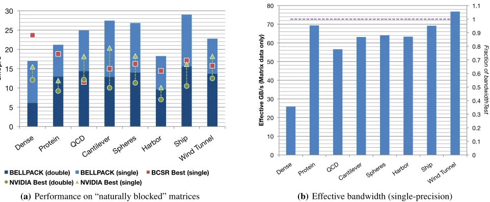
The performance results for BELLPACK format appear in Fig-ures 5(a) (Gflop/s for single- and double-precision) and 5(b) (esti-mated effective GB/s in single-precision). We show results on just the subset of matrices which actually have dense block substruc-ture; for the remainder, we would expect the best NVIDIA imple-mentation to deliver the best results.
By “estimated effective bandwidth,” we mean the best perfor-mance one would expect given (a) an effective sustainable band-width as given by the CUDA SDK bandwidthTestbenchmark, shown in Table 1; and (b) an optimistic flop:byte ratio of 2 flops for every 4 bytes read, which accounts only for the minimum mem-ory traffic required just to transfer the matrix values (i.e., assuming the “maximum index compression” possible). For example, on the NVIDIA C1060, we observe abandwidthTestmeasurement of 72 GB/s, which corresponds to an estimated empirical peak perfor-mance of (72 GB/s)×(2 flops / 4 bytes) = 36 Gflop/s.
Figure 5 show the best performance found by exhaustively searching through 11 different blocking sizes and 4 different thread block sizes and choosing the best results. Similarly, the “NVIDIA Best” implementation is that of Bell and Garland, showing the best result that we observed over all of the formats available in their implementation [3]. Our BELLPACK implementation is between 1.3×to 1.8×faster for single-precision, and between 1.1×to 1.5× faster for double-precision, achieving a bandwidth utilization that approaches the peak measured bandwidth.
6.
Model-based Autotuning
Achieving the best performance from BELLPACK requires care-fully tuning the block size parameters,r,c, andR. These param-eters are matrix-dependent, meaning we may need to choose them at run-time. In the spirit of our prior work, we select these param-eters using an autotuning framework based on empirical model-ing [11, 19, 22]. This model combines off-line benchmarkmodel-ing and a run-time model instantiated with the benchmark data. In contrast to this prior SpMV autotuning work, our model attempts to more directly model GPU hardware features, rather than abstracting the hardware away completely [11, 19].
6.1 A Generic Model of GPU Execution Time
Our model is based on a simple abstraction of an NVIDIA GPU architecture and its execution model, illustrated in Figure 6.
Basic model: Iterations. We consider a GPU as consisting ofM
0
5
10
15
20
25
30
Dense
Protein
QCD
Cantilever
Spher es
Harbor
Ship
Wind T unnel
Gflop/s
BELLPACK (double) BELLPACK (single) BCSR Best (single)
NVIDIA Best (double) NVIDIA Best (single)
(a)Performance on “naturally blocked” matrices
0
0.1
0.2
0.3
0.4
0.5
0.6
0.7
0.8
0.9
1
1.1
0
10
20
30
40
50
60
70
80
Dense
Protein
QCD
Cantilever
Spher es
Harbor
Ship Wind T
unnel
Fraction of bandwidthT
est
Ef
fective GB/s (Matrix data only)
(b)Effective bandwidth (single-precision) Figure 5. BELLPACK performance on NVIDIA C1060 (T10P multiprocessor)
GPU
CROSSBAR
DRAM
Bank DRAMBank
...
DRAMBank...
SM #1 SM #2 SM #3 SM #M
Workload L
...
...
I Workload L
T
M
Figure 6. A diagram of NVIDIA GPU architecture and execution model
blocks. Importantly,Tdepends on characteristics of both the hard-ware and the compute kernel (e.g., via the so-calledoccupancy); we discuss how to computeTin Section 6.2 below.
We model the GPU’s execution as all SMs executing its thread blocks initerations. During each iteration, an individual SM exe-cutes up toTthread blocks that it has been assigned.
If the computational workload consists of a total ofLthread blocks, we can compute the total number of iterationsIunder some assumptions. Let us assume that the SMs are “perfectly synchro-nized” in the sense that, during a given iteration, all SMs on thread blocks consisting of identical work can proceed in close unison. Then, during each iteration, allMSMs will execute up toTthread blocks each, meaning the total number of such iterations is
I=
‰ L
T×M
ı
. (1)
We consider the total execution time to be the sum of the execution times of the individual iterations. Under the assumption
of roughly identical work during an iteration, the total timetis
t=
I X
i=1
ti (2)
wheretiis the time of each iteration. We model this iteration time using a simple linear function of the maximum number of thread blocks,k, assigned to any SM during iterationias follows:
ti(k) =σi+αi×(k−1), (3)
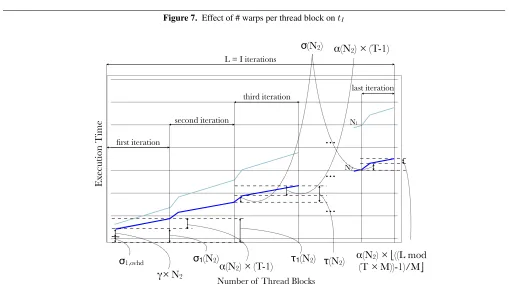
where1≤ k ≤ T;σimodels the iteration’s startup time, which includes some overhead plus the time to compute the first iteration; andαimeasures the degree to which the SM can hide the latency of each thread block through context switching. The first iteration’s startup cost,σ1, could include things like the kernel startup time. Regarding the latency hiding, the smaller the value ofαi, the better the SM is able to hide the thread block latency.
Homogeneous execution. For the kernels we consider in this pa-per, we make an additional simplification. Suppose that the thread blocks are largely homogeneous in the sense thatαi = αis the same for all iterations and that only the first iteration may have a different overhead term, i.e.,σ2=σ3=· · ·=σI=σbutσ1may or may not equalσ. Then, assumingI ≥2, we can write the total time in three terms, namely, the timeτ1for the first iteration, the timeτ for each of the middleI−2iterations, and the timeτIfor the last iteration:
t = τ1+ (I−2)×τ+τI (4)
τ1 = σ1+α×(T−1) (5)
τ = σ+α×(T−1) (6)
τI = σ+α×
—
(L mod (T×M))−1 M
. (7)
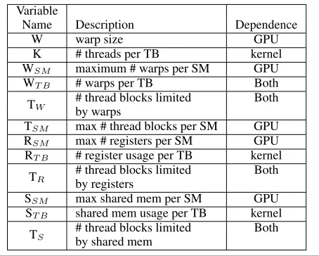
Variable
Name Description Dependence
W warp size GPU
K # threads per TB kernel
WSM maximum # warps per SM GPU
WT B # warps per TB Both
TW # thread blocks limited Both by warps
TSM max # thread blocks per SM GPU
RSM max # registers per SM GPU
RT B # register usage per TB kernel
TR # thread blocks limited Both by registers
SSM max shared mem per SM GPU
ST B shared mem usage per TB kernel
TS # thread blocks limited Both by shared mem
Table 3. Table of variables used to calculateT
be much larger than the cost of computing the subsequent thread block. This skew will depend on kernel features such as the num-ber memory operations and the numnum-ber of warps in a single thread block and hardware factors such as the bandwidth and the number of banks in the memory system [10]. We illustrate this phenomenon in Figure 7.
Illustration of the model. The overall execution model described in this section can be summarized graphically, as shown in Figure 8.
6.2 ComputingT(Max. Thread Blocks per Multiprocessor) The execution time model of Section 6.1 assumes that at mostT
thread blocks (TBs) can co-exist on the same SM. This value, which is related to the CUDA’s kernel occupancy [1], can be computed for a given GPU and kernel using Equations 8 through 12 below. These equations depend on a number of GPU- and kernel-dependent parameters, which are summarized in Table 3.
WT B =
K
W (8)
TW = min
„ TSM,
—
WSM
WT B «
(9)
TR =
—
RSM
RT B
(10)
TS =
— SSM ST B
(11)
T = min(TW, TR, TS) (12)
6.3 Instantiating the Model for SpMV
To use the model for autotuning SpMV, we need to instantiate an SpMV-specific model. Like related work, we use offline bench-marking [11, 19], but in contrast, we use this data to determine various parameters in the model (e.g.,σ,α). In this section, we in-stantiate a model for the BELLPACK kernel, using the homogenous model (Section 6.1).
Computing the startup cost,σi. All of the BELLPACK kernels (one for each value of r and c) have the same structures. For instance, the kernels all load thread block related data such as the thread and block ID; index into the main data structures; and declare variables. The main portion of the kernel loops over all ther×cblocks that the thread block is assigned and computes
the necessary values. The kernel ends by copying the accumulated values back to the vectorY.
The first iteration’s startup cost,σ1, is mainly determined by the number ofr×cblocks it reads. For ar×ckernel of thread block sizeR, where each thread processesNblocks of sizer×ceach,
σ1andσcan be approximated as follows:
σ1(N) = σ1,o+γ×N (13)
σ(N) = γ0×N . (14)
Observe that Equation 13 further decomposes theσ1startup into a “base” overhead,σ1,o plus the timeγ×Nto process theNblocks. We determine the various factors in Equations 13–14 using of-fline benchmarks on dense matrices. Specifically, we first estimate
σ1,o by measuring the time to execute the kernel on a(M×R×r) -by-cdense matrix stored in BELLPACK format. We then execute the kernel on a(M ×R×r)-by-(c×β)dense matrix, for some value ofβ(below), and measure its execution time,φM·R·r×c·β. From these data, we determineγvia
γ= (φM·R·r×c·β−σ1,o)
β . (15)
We compute the subsequent iteration times,γ0, as follows:
γ0= (φM·(T+1)·R·r×c·β−φM·T·R·r×c·β)
β (16)
The valueβcan be chosen arbitrarily, but should be kept small (≤ 100).
Estimating the latency-hiding factor,α. The variableαis used to estimate the increase in the execution time as additional thread blocks are added to the SM, and its value reflects the ability to hide latency (Section 6.1). We estimateαby
α(N) = „
φM·T·R·r×c·β−φM·R·r×c·β (T−1)×β
«
×N, (17)
using previously estimated values.
Final execution time model. The preceeding benchmarks are enough to estimate the execution time for a particularr×ckernel with thread block sizeR and N BELLPACK blocks as shown below, again assumingI ≥ 2. Having the equation vary withN
creates a more flexible model and estimates the range of errors that may occur due to variance in blocking size estimation, discussed in a subsequent section.
τ1(N) = σ1(N) +α(N)×(T−1) (18)
τ(N) = σ(N) +α(N)×(T −1) (19)
τI(N) = σ(N) +α(N)×
—
(L mod (T×M))−1 M
(20)
t(N) = τ1(N) + (I−2)τ(N) +τI(N) (21)
6.4 Blocking Size Estimation
As SpMV is a bandwidth limited application, one simple way of eliminating potential blocking sizes is to estimate the total amount of data that would be generated by using those sizes. For exam-ple, for the “Protein” matrix, a blocking size of 3×3 generates 4.9M data elements on average, approximately 1.13×more data elements than the original matrix, whereas blocking sizes of 7×7 and 8×8 generate 2.1×and 2.2×more data respectively. Since 7×7 and 8×8 blocking sizes produce significantly more data, they can be safely eliminated from consideration as long as they can be roughly estimated.
Memory Op Arithmetic Op
1 Thread Block 2 Thread Block 4 Thread Block
1 warp/ TB
10 + 1 = 11 cycles
10 + 2 = 12 cycles
10+ 4 = 14 cycles
4 warp/ TB
10 + 4 = 14 cycles
...
10 + 8 = 18 cycles
...
10 + 16 = 26 cycles
0 5 10 15 20 25 30
0 1 2 4
Ex
ec
u&
on Tim
e (c
yc
le
s)
# Thread Blocks Processed
1 warp/TB 4 warp/TB
Figure 7. Effect of # warps per thread block ontI
σ
1,ovhdγ×
N2
σ
1(N2)...
...
...
first iterationlast iteration
second iteration
third iteration
α(N2)
×
(T-1)
τ
1(N2)N1
N2
L = I iterations
α(N2)
×
(T-1)
τ
(N2)
α(N2)
(T ×
M))-1)/M
×
⎣
((L mod
⎦
Ex
ec
ut
ion
T
im
e
Number of Thread Blocks
σ
(N2)
Figure 8. Execution Model Graph
relatively accurately measure the ratio of number of stored values to the number of non-zeros by sampling only 1% of the matrix.
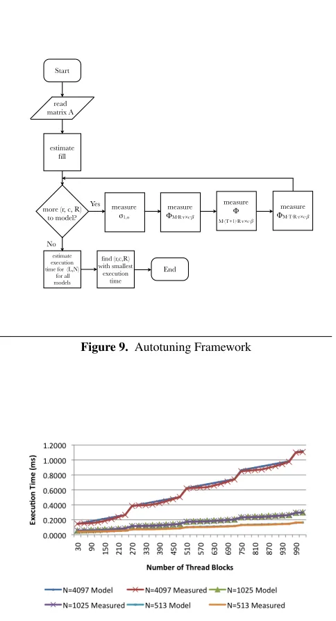
6.5 Autotuning Framework
Once a list of potential optimal blocking sizes has been created, we can use the equations described in the previous sections to compute the models for the different blocking sizes and thread block size R. A flowchart showing the process is shown in Figure 9.
The framework is flexible as many of these parameters can be fine-tuned to suit the needs of the application. For example, the size of the list of potential blocking sizes can be controlled by tightening the range of total data size allowed, and if certain thread block sizes result in consistently poor performance numbers, those can skipped.
6.6 Experimental Results
Dense matrix in sparse format. As partial validation of the model, we compare the model predictions against measurements for a dense matrix in BELLPACK format, shown in Figures 10–12. These measurements are taken on two different GPUs with very different hardware specs to verify that the functional form of the model was not specifically tied to either one of the GPUs.
The model estimates the performance closely with average and median error of 3.74% and 2.73% respectively, and maximum error of 14.89% for the 1×2 kernel for R=32. The 3×3 kernel for
0 0.1 0.2 0.3 0.4 0.5 0.6
30 90 150 210 270 330 390 450 510 570 630 690 750
Ex
ec
u&
on Tim
e (m
s)
Number of Thread Blocks
N=10 Model N=10 Measured N=50 Model N=50 Measured N=100 Model N=100 Measured
0 1 2 3 4 5
30 90 150 210 270 330 390 450 510 570 630 690 750
Ex
ec
u&
on Tim
e (m
s)
Number of Thread Blocks
N=100 Model N=100 Measured N=50 Model N=50 Measured N=10 Model N=10 Measured
Figure 10. Comparison of model to real data for BELLPACK on T10
Start
read matrix A
estimate fill
more (r, c, R) to model?
No Yes
estimate execution time for (L,N)
for all models
find (r,c,R) with smallest
execution time
End measure
σ1,o
measure ΦM⋅R⋅r×c⋅β
measure Φ M⋅(T+1)⋅R⋅r×c⋅β
measure ΦM⋅T⋅R⋅r×c⋅β
Figure 9. Autotuning Framework
Figure 11. Comparison of model to real data for BCSR on T10
0 0.05 0.1 0.15 0.2 0.25 0.3 0.35 0.4 0.45
16 32 48 64 80 96 112 128 144 160 176 192 208 224 240 256 272
Ex
ec
u&
on Tim
e (m
s)
Number of Thread Blocks
N=100 Model N=100 Measured N=50 Model N=50 Measured N=10 Model N=10 Measured
Figure 12. Comparison of model to real data for BELLPACK on C870
The same model was tested on a Tesla C870 also, which has a different number of SM and hardware resources. Figure 12 shows that the same performance model works across different hardware. The average and median error rates were 2.18% and 2.06% respec-tively, and the maximum error was 6.18%.
Tests on the matrix suite. The results obtained by autotuning as compared to the best performance found by exhaustive search is shown in Figure 13. Since BELLPACK is designed only for matri-ces with dense block substructure, we evaluate only against those 8 matrices. Such structure can be quickly and easily detected [19]. Figure 13 shows that we find near-optimal block sizes in 5 of 8 cases, with the non-optimally tuned kernels achieving 86.5% of the best performance numbers on average (median of 92.6%).
The autotuning was done over 1×2, 2×2, 2×3, 3×2, 3×3, 3×4, 4×4, 5×5, 6×6, 7×7, and 8×8 kernels, forRsizes of 32, 64, 128, and 256 each, a total of 44 possible combinations. Some blocking sizes such as 7×7 and 8×8 were eliminated by fill estimation for most matrices, as they yielded extremely large data sizes.
An 86.5% average accuracy (92.6% median) relative to exhaus-tive search leaves room for improvement. Nevertheless, even for the worst mispredictions, the performance of the selected optimization is still at least as fast as the best NVIDIA implementation.
6.7 Alternatives to our model-based approach
10.8
19.1 23.8 24.6 25.3
12.2 22.2 16.1
0% 10% 20% 30% 40% 50% 60% 70% 80% 90% 100%
Dense
Protein
QCD Cantilever
Spheres
Harbor
Ship
Wind T unnel
Autotuned Exhaustive
Figure 13. Performance of the implementation found using our au-totuning model, as a fraction of the performance of the implemen-tation found by exhaustive search. The numerical values on each bar indicate the Gflop/s of the autotuned implementation.
reasonably expect the optimal block size to be the one that min-imizes the matrix data structure footprint. However, in our ex-haustive search-based experiments, we found this heuristic to yield mixed results. The main cause is is that this heuristic ignores the actual kernel performance, since each data structure we consider has an associated kernel computation, and that kernel performance can vary widely and in unintuitive ways depending on register al-location, alignment, and other issues.
7.
Conclusions and Future Work
Our findings lend further support to the intuition that a memory bandwidth-rich GPU platform can deliver excellent absolute per-formance on SpMV, at least for the class of matrices with dense block substructure, such as those arising in finite element method applications. The absolute performance numbers we achieve are among the best published thus far across a wide spectrum of single-node multisocket multicore platforms, including prior GPU SpMV results [2, 3] and the STI Cell Broadband Engine [21].
To make our BELLPACK-based SpMV practical, however, re-quires a judicious choice of data structure tuning parameters, a problem not addressed in prior GPU SpMV work. We contribute a GPU-specific execution time model, inspired by the general CUDA programming model, that can accurately predict suitable tuning pa-rameters. The main limitation of our study is that we have thus far only validated it with respect to our BELLPACK and BCSR SpMV implementations on GPUs. However, as part of our on-going work, we continue to validate and refine the model on additional kernels. We believe that with the appropriate level of additional refinement, we could provide insight into the performance of more general GPU-like architectures, providing both a way to “tune” an archi-tecture via modeling as well as providing an analytical modeling tool for designing algorithms and their implementations.
Acknowledgments
This work was supported in part by the National Science Founda-tion (NSF) under award number 0833136, NSF TeraGrid alloca-tion CCR-090024, joint NSF 0903447 / Semiconductor Research Corporation (SRC) Award 1981, and a grant from the Defense Ad-vanced Research Projects Agency (DARPA). Any opinions,
find-ings and conclusions or recommendations expressed in this mate-rial are those of the authors and do not necessarily reflect those of NSF, SRC, or DARPA.
References
[1] NVIDIA CUDA (Compute Unified Device Architecture): Program-ming Guide, Version 2.1, December 2008.
[2] Muthu Manikandan Baskaran and Rajesh Bordawekar. Optimizing sparse matrix-vector multiplication on GPUs using compile-time and run-time strategies. Technical Report RC24704 (W0812-047), IBM T.J. Watson Research Center, Yorktown Heights, NY, USA, December 2008.
[3] Nathan Bell and Michael Garland. Efficient sparse matrix-vector multiplication on CUDA. InProc. ACM/IEEE Conf. Supercomputing (SC), Portland, OR, USA, November 2009. (to appear).
[4] Jeff Bolz, Ian Farmer, Eitan Grinspun, and Peter Schr¨oder. Sparse matrix solvers on the GPU: Conjugate gradients and multigrid. In Proc. Special Interest Group on Graphics Conf. (SIGGRAPH), San Diego, CA, USA, July 2003. doi: http://dx.doi.org/10.1145/882262.882364.
[5] Matthias Christen and Olaf Schenk. Genera-purpose sparse matrix building blocks using the NVIDIA CUDA technology platform. InProc. Workshop on General-Purpose Processing on Graphics Processing Units (GPGPU), Boston, MA, USA, October 2007. [6] Eduardo F. D’Azevedo, Mark R. Fahey, and Richard T. Mills.
Vectorized sparse matrix multiply for compressed row storage. In
Proc. Int’l. Conf. Computational Science (ICCS), volume 3514/2005 ofLNCS, pages 99–106. Springer Berlin / Heidelberg, 2005. doi: http://dx.doi.org/10.1007/11428831 13.
[7] James Demmel, Jack Dongarra, Viktor Eijkhout, Erika Fuentes, Antoine Petitet, Richard Vuduc, R. Clint Whaley, and Kather-ine Yelick. Self-adapting linear algebra algorithms and soft-ware. Proc. IEEE, 93(2):293–312, February 2005. doi: http://dx.doi.org/10.1109/JPROC.2004.840848.
[8] Michael Garland. Sparse matrix computations on many-core GPUs. In Proc. ACM/IEEE Design Automation Conf. (DAC), pages 2–6, Anaheim, CA, USA, 2008. doi: http://dx.doi.org/10.1145/1391469.1391473.
[9] Roman Geus and Stefan R¨ollin. Towards a fast sparse symmetric matrix-vector multiplication. Parallel Computing, 27(7):883–896, June 2001. doi: http://dx.doi.org/10.1016/S0167-8191(01)00073-4. [10] Sunpyo Hong and Hyesoon Kim. An analytical model for
a GPU architecture with memory-level and thread-level paral-lelism awareness. In Proc. ACM Int’l. Symp. Comp. Arch. (ISCA), pages 152–163, Austin, TX, USA, June 2009. doi: http://dx.doi.org/10.1145/1555815.1555775.
[11] Eun-Jin Im, Katherine Yelick, and Richard Vuduc. SPARSITY: Optimization framework for sparse matrix kernels. Int’l J. of High Performance Computing Applications (IJHPCA), 18(1):135–158, February 2004. doi: http://dx.doi.org/10.1177/1094342004041296. [12] Hiroshi Okuda, Kengo Nakajima, Mikio Iizuka, Li Chen, and Hisashi
Nakamura. Parallel finite element analysis platform for the Earth Simulator: GeoFEM. InProc. Int’l. Conf. Computational Science (ICCS), volume 2659 ofLNCS, pages 773–780. Springer, 2003. doi: http://dx.doi.org/10.1007/3-540-44863-2 75.
[13] Ali Pinar and Michael T. Heath. Improving performance of sparse matrix-vector multiplication. In Proc. ACM/IEEE Conf. Supercomputing (SC), Portland, OR, USA, 1999. doi: http://dx.doi.org/10.1145/331532.331562.
[14] John R. Rice and Ronald F. Boisvert.Solving elliptic problems using ELLPACK. Springer Verlag, 1984.
[15] Yousef Saad. SPARSKIT: A basic tool kit for sparse matrix computations, version 2.
http://www-users.cs.umn.edu/ saad/software/SPARSKIT /sparskit.html, March 2005.
SIGGRAPH/EUROGRAPHICS Symp. Graphics Hardware, San Diego, CA, USA, 2007.
[17] Vasily Volkov and James W. Demmel. Benchmarking GPUs to tune dense linear algebra. InProc. ACM/IEEE Conf. on Supercomputing (SC), Austin, TX, USA, November 2008.
[18] Richard Vuduc, James W. Demmel, and Katherine A. Yelick. OSKI: A library of automatically tuned sparse matrix kernels. InProc. SciDAC, J. Phys.: Conf. Series, volume 16, pages 521–530, 2005. doi: http://dx.doi.org/10.1088/1742-6596/16/1/071.
[19] Richard W. Vuduc. Automatic performance tuning of sparse matrix kernels. PhD thesis, University of California, Berkeley, CA, USA, January 2004.
[20] Richard W. Vuduc and Hyun-Jin Moon. Fast sparse matrix-vector multiplication by exploiting variable block structure. InProc. High-Performance Computing and Communications Conf., volume LNCS 3726/2005, pages 807–816, Sorrento, Italy, September 2005. Springer. doi: http://dx.doi.org/10.1007/11557654 91.
[21] Sam Williams, Richard Vuduc, Leonid Oliker, John Shalf, Katherine Yelick, and James Demmel. Optimizing sparse matrix-vector multiply on emerging multicore platforms. Jour-nal of Parallel Computing, 35(3):178–194, March 2009. doi: http://dx.doi.org/10.1016/j.parco.2008.12.006.