Integration of optical and SAR remote sensing images for crop-type
mapping based on a novel object-oriented feature selection method
Jintian Cui
1,2,
Xin Zhang
1*,
Weisheng Wang
3,
Lei Wang
1(1. State Key Laboratory of Remote Sensing Science, Aerospace Information Research Institute, Chinese Academy of Sciences, Beijing 100101, China; 2. University of Chinese Academy of Sciences, Beijing 100049, China;
3. Xinjiang Institute of Ecology and Geography, Chinese Academy of Sciences, Urumqi 830011, China)
Abstract: Remote sensing is an important technical means to investigate land resources. Optical imagery has been widely used in crop classification and can show changes in moisture and chlorophyll content in crop leaves, whereas synthetic aperture radar (SAR) imagery is sensitive to changes in growth states and morphological structures. Crop-type mapping with a single type of imagery sometimes has unsatisfactory precision, so providing precise spatiotemporal information on crop type at a local scale for agricultural applications is difficult. To explore the abilities of combining optical and SAR images and to solve the problem of inaccurate spatial information for land parcels, a new method is proposed in this paper to improve crop-type identification accuracy. Multifeatures were derived from the full polarimetric SAR data (GaoFen-3) and a high-resolution optical image (GaoFen-2), and the farmland parcels used as the basic for object-oriented classification were obtained from the GaoFen-2 image using optimal scale segmentation. A novel feature subset selection method based on within-class aggregation and between-class scatter (WA-BS) is proposed to extract the optimal feature subset. Finally, crop-type mapping was produced by a support vector machine (SVM) classifier. The results showed that the proposed method achieved good classification results with an overall accuracy of 89.50%, which is better than the crop classification results derived from SAR-based segmentation. Compared with the ReliefF, mRMR and LeastC feature selection algorithms, the WA-BS algorithm can effectively remove redundant features that are strongly correlated and obtain a high classification accuracy via the obtained optimal feature subset. This study shows that the accuracy of crop-type mapping in an area with multiple cropping patterns can be improved by the combination of optical and SAR remote sensing images.
Keywords: crop-type mapping, synthetic aperture radar (SAR), high-resolution remote sensing, image segmentation, feature subset selection, object-oriented classification
DOI: 10.25165/j.ijabe.20201301.5285
Citation: Cui J T, Zhang X, Wang W S, Shen Y. Integration of optical and SAR remote sensing images for crop-type mapping based on a novel object-oriented feature selection method. Int J Agric & Biol Eng, 2020; 13(1): 178–190.
1 Introduction
Mapping regional and global cropland distribution in a timely manner is a main basis for crop yield estimation, crop growth monitoring and acreage surveys[1,2]. With the ability to quickly and efficiently collect information in real time over wide ranges, remote sensing is a rich data source for crop-type mapping[3]. Multiresolution or multitemporal optical images with abundant spectral and texture information have been widely used in crop identification[4-6]. However, data acquisition of optical remote sensing images will inevitably be affected by clouds and rain. Due to the limitation of optical images for discrimination of crops with similar spectra, the accuracy of crop classification with a single optical image may be reduced.
Radar remote sensing mainly acquires images, which are
Received date: 2019-07-13 Accepted date: 2019-11-20
Biographies: Jintian Cui, Master degree candidate, research interests: agricultural remote sensing, machine learning and SAR, Email: [email protected];
Weisheng Wang, PhD, Researcher, research interests: high-resolution remote sensing and SAR, Email: [email protected]; Lei Wang, PhD, research interests: digital earth and inernet GIS, Email: [email protected].
*Corresponding author: Xin Zhang, PhD, Researcher, research interests: agricultural remote sensing and spatial analysis. Mailing address: A3, Datun Road, Chaoyang District, Beijing 100101, China. Tel: +86-10-64887892, Email: [email protected].
C-band RADARSAT-2 dataset to evaluate five decomposition techniques based on incoherent and coherent decompositions as well as the radar vegetation index (RVI) for crop classification over heterogeneous agricultural areas. Among the incoherent models, Freeman 3-component decomposition was found to perform better in distinguishing vegetation from other land covers. Jiao[20] applied the polarimetric parameters extracted from Cloude–Pottier and Freeman–Durden decompositions to SAR crop mapping, and object-oriented classification results derived from a single date of PolSAR image indicated an overall accuracy of 95% and a Kappa of 0.93, which was a 6% improvement over linear-polarization only classification.
Due to the different characteristics of SAR and optical remote sensing in imaging mechanisms, the combination of radar and multispectral data has become one of the trends in agricultural remote sensing. Several studies verified that higher mapping accuracies can be reached by combining the two data sources[21-23]. Steinhausen et al.[24] applied a random forest-based wrapper approach to select the most relevant SAR images for combining with optical images, and the results indicated that combining Sentinel-1 and Sentinel-2 data can improve land cover mapping in cloud-prone regions. De Alban et al.[25] created image stacks from
the Landsat and SAR layers and delineated regions of interest to map land cover using a random forest classifier, indicating that the combined use of Landsat and L-band SAR data was superior to individual sensor data. Fusing optical and SAR data has been given more attention in numerous studies and were employed on three levels: the pixel level, the feature level and the decision level. However, due to speckle noise inherent in SAR imagery, pixel-level fusion is inappropriate for SAR data[26]. Hong et al.[27] noted that some methods, such as high-pass filters (HPFs), wavelet transforms and contourlet transforms, can retain texture information, but high-frequency information and spatial details derived from SAR images were lost. Feature-level fusion is usually implemented on features extracted from images. Perushan et al. [28] adopted feature-level image fusion to fuse Sentinel-2 and Landsat 8 images with SAR images and discriminated an alien plant species from its surroundings using a support vector machine (SVM) supervised classification algorithm, but the classification accuracy needs to be improved. Because of the inherent noise in SAR data and different imaging models between optical and SAR data, fusion methods between two heterogeneous images are difficult to perform.
Speckle noise resulting from the coherent imaging system of SAR affects the image quality and interpretation, reducing the classification accuracy derived from the pixel-based classification methods[29]. Object-oriented classification, as a novel classification approach, can extract features, such as texture, shape and spatial information, after image segmentation which would suppress noise and improve the classification accuracy[30]. Some
statistical models and segmentation methods for SAR data have been studied[31-33]. However, due to the high dynamics and local statistical properties of SAR images, there are still limitations in SAR image segmentation. Therefore, a feasible solution, that is, image segmentation based on high-resolution optical imagery, could accurately express the ground information and avoid salt-and-pepper noise in image processing.
To make full use of the advantages of optical and SAR images, a scheme has been developed for crop-type mapping using GaoFen-2 (GF-2) optical images and GaoFen-3 (GF-3) PolSAR
images. In total, 58 feature parameters related to crop growth were extracted from optical and SAR images, and object-oriented crop classification was performed with the support of farmland parcels segmented from the high-resolution GF-2 image. Furthermore, a novel feature selection algorithm that is based on within-class aggregation and between-class scatter is proposed to extract the optimal feature subset and is abbreviated WA-BS. To utilize and evaluate the complementary advantages of the multisensory method, our main objectives are (1) to test the validity of the combination of GF-2 and GF-3 data for crop-type mapping with the support of farmland parcels derived from optical image segmentation and (2) to quickly select the optimal feature subset from remote sensing images and evaluate the contribution of each feature during the crop growth stage. An experiment was carried out in an agricultural district within Xinjiang Uygur Autonomous Region, China, to examine the feasibility of the proposed method.
2 Study area and datasets
2.1 Study area
The study area is located in an agricultural district stretching over Bohu and Yanqi counties of Xinjiang Uygur Autonomous Region that faces Bosten Lake to the east, which is the largest inland freshwater lake in China. This area is one of the most productive agricultural regions in Xinjiang Uygur Autonomous Region, mainly for food crops (maize and winter wheat) and economic crops (tomatoes, beets, cotton and fruit). The geographic extent of the study area is shown in Figure 1. This region has a dry, temperate continental climate. The annual precipitation is approximately 79.2 mm, and the annual evaporation ranges from 1800 to 2000 mm. Due to the multiple crop types and a unique crop calendar, this area is ideal to examine the potential for the combined use of optical and SAR remote sensing images for mapping crops.
Figure 1 Study site in the agricultural area of Xinjiang Uygur Autonomous Region, China
2.2 Remote sensing data and preprocessing
preprocessing of the GF-2 data was performed in ENVI 5.3, including radiation calibration, atmospheric correction and geometric correction. Radiometric calibration was performed by using the absolute radiation calibration coefficient of the GF-2 data provided by CRESDA. Atmospheric correction was carried out using the second simulation of the satellite signal in the solar spectrum (6S) model[37]. Geometric correction was based on a WorldView-2 image with accurate spatial coordinate information. A quadratic polynomial correction algorithm was utilized by adding group control points (GCPs), and the error was controlled within 0.5 pixels. In the 1-m fusion image, farmland boundaries could be clearly represented on the GF-2 images, guaranteeing the extraction of the farmland parcels.
The GF-3 satellite, the first Chinese C-band civil radar satellite, has 12 imaging modes with a fine spatial resolution up to 1 m and was launched on 10 August 2016. The GF-3 PolSAR data of quad-polarization strip I (QPSI) mode with a spatial resolution of 8 m were downloaded from the CRESDA website. According to field investigations, the crop types in the study area were mainly wheat, cotton, maize, beets and tomatoes. Considering the phenological characteristics of the crops (Figure 2), GF-3 data from 6 July 2018 were utilized to classify the crop types. At this time, the crop growth characteristics were significantly different. The SAR data were preprocessed in Pixel Information Expert (PIE), including radiometric calibration, multi-look processing, refined Lee filtering (window size of 5×5)[38] and geometric correction. GCPs were used to coregister the GF-3 image and the preprocessed GF-2 image until the error was less than 0.5 pixels.
Figure 2 Crop calendar for the study site 2.3 Field data collection
The sample data were collected in mid-July 2018 during fieldwork. With a land use map of the study area and a Google Earth image from this period as reference maps, the random clustered sampling approach[39] was used to obtain the samples. The sampling method first randomly selected certain groups that were non-crossing and non-repeating in the study area, then randomly selected several clusters from the groups and investigated all the individuals or units in these clusters. Then, a simple random sampling method was used to select a certain class in the cluster as the sample to be collected. Each cluster was a geographical area, which was used as an investigation unit. A Trimble Pro XRT GPS receiver with a positioning accuracy of 0.2 m was used to mark the geographical coordinates (latitude and longitude) of these samples, and geotagged photos were taken at each site to record the sample types. In addition, the field data also contained other land cover information, including water bodies, residential areas, woodlands, wetlands and bare land. To train the classification model and investigate the crop classification accuracy, we randomly divided the crop samples into 3224 training samples and 1470 validation samples, as shown in Table 1.
Table 1 Training and validation samples of each crop class
Class Training samples Validation samples
Wheat 589 257
Maize 564 252
Cotton 635 283
Beets 691 340
Tomatoes 745 338
3 Methodology
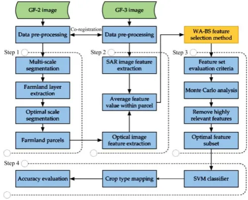
The four-step procedure for crop-type mapping with the combined use of optical and SAR remote sensing images is outlined in Figure 3: (1) acquire the map layer of the farmland parcels at the optimal segmentation scale, which is used to classify crop types at parcel level; (2) extract multiple polarimetric features from the SAR image and the texture features and vegetation index from the optical image; (3) select the optimum feature set from high-dimensional features through the WA-BS algorithm proposed in this paper; and (4) use the support vector machine one-versus-rest (SVM-OVR) algorithm to perform object-oriented classification with the support of the farmland parcels segmented from high-resolution optical image.
Figure 3 Overview of the methodology for mapping crops with the combined use of optical and SAR remote sensing images 3.1 Farmland parcel extraction from an optical image
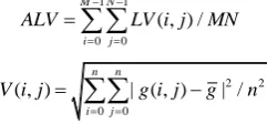
In the process of image segmentation, the segmentation scale greatly affects the spatial structure of the objects. Therefore, it is important to set the optimal scale so that the homogenous pixels with similar spectral characteristics, brightness and texture can be classified as the same object. In this study, we used the local variance method[40,41] to select the optimal scale of farmland and resegmented the farmland layer. The local variance in the window was calculated by a moving window of size n×n pixels, and then the average local variogram (ALV) map was generated, as shown in Equation (1). The range for the ALV curve was determined by the change rate in the ALV with the segmentation scale. In fact, the extreme point or critical point of the local variance cannot be found mathematically. Therefore, the threshold of the change rate in the ALV should be set according to the experiment. As the segmentation scale increases, the scale that corresponds to the point whose change rate is initially less than the threshold is the optimal segmentation scale of the farmland parcels.
1 1
0 0
( , ) /
M N
i j
ALV LV i j MN
(1)2 2
0 0
( , ) | ( , ) | /
n n
i j
LV i j g i j g n
where, M and N represent the number of rows and columns of the image, respectively; i and j are the row and column numbers in the local window, respectively; LV(i, j) is the local variance of the i-th row and j-th column pixel; g(i, j) is the gray value of the pixel, and
g is the mean of the gray values with the local window. 3.2 Feature extraction from multisource images 3.2.1 SAR image feature extraction
Features derived from polarimetric decomposition and the radar indices have physical meanings and are sensitive to crop growth stages[42]. Polarimetric decomposition is helpful for revealing the physical mechanism of scatters by using a polarimetric scattering matrix, such as a covariance matrix, a coherence matrix or a scattering matrix. A number of polarimetric decomposition theories have been proposed, including coherent target decomposition and incoherent target decomposition. The various parameters derived from SAR polarimetric decomposition reflect the scattering difference between the target and the background from different angles, which is helpful for accurately identifying crop targets via the joint use of these parameters. In this study, we extracted three types of features from the SAR imagery: (1) features based on the original PolSAR data (i.e., the Sinclair scattering matrix, coherent matrix and covariance matrix were calculated for the full-polarized image to extract the original matrix parameters); (2) features based on different polarimetric decomposition theories, including Cloude-d[43], Freeman-d[44], VanZyl-d[45], Krogager-d[46], Pauli decomposition[47] (Pauli-d), Barnes-d[48], Holm-d[49], Yamaguchi-d[50], Huynen-d[51], Neumann-d[52] and H/A/Alpha-d[53]; and (3) features including the total scattering power SPAN of the Sinclair scattering matrix, the radar vegetation index (RVI), and the pedestal height (PH). In total, 50 parameters were extracted, as shown in Table 2.
Table 2 Features extracted from the PolSAR data for crop-type mapping
Feature class Method Feature parameter N-parameters
Original features
Sinclair scattering matrix (1) S1 (2) S2 (3) S3 3
Coherence matrix (4) T1 (5) T2 (6) T3 3
Covariance matrix (7) C1 (8) C2 (9) C3 3
Polarimetric Decomposition
features
Freeman (10) Freeman-Vol (11) Freeman-Odd (12) Freeman-Dbl 3
Krogager (13) Krogager-KS (14) Krogager-KD (15) Krogager-KH 3
van Zyl (16) VanZyl-Vol (17) VanZyl-Odd (18) VanZyl-Dbl 3
Barnes (19) Barnes-T11 (20) Barnes-T22 (21) Barnes-T33 3
Pauli (22) Pauli-a (23) Pauli-b (24) Pauli-c 3
Cloude (25) Cloude-T11 (26) Cloude-T22 (27) Cloude-T33 3
Holm (28) Holm-T11 (29) Holm-T22 (30) Holm-T33 3
Yamaguchi (31) Yamaguchi-Vol (32) Yamaguchi-Odd (33) Yamaguchi-Dbl 4 (34) Yamaguchi-Hlx
Huynen (35) Huynen-T11 (36) Huynen-T22 (37) Huynen-T33 3
Neumann (38) Neumann-dela-mod (39) Neumann-dela-pha 2
H/A/Alpha (40) Alpha Angle (41) A (Anisotropy) (42) H (Entropy) 3
SAR discriminators
(43) RVI (Radar Vegetation Index)
8 (44) PF (Polarization Fraction)
(45) PH (Pedestal Height) (46) PA (Polarization Asymmetry) (47) SE (Shannon Entropy)
(48) DERD (Double-bounce Eigenvalue Relative Difference) (49) SERD (Single-bounce Eigenvalue Relative Difference) (50) SPAN
3.2.2 Optical image feature extraction
The texture features derived from optical images are helpful for distinguishing different objects compared with classification with pure spectral features only[54]. The commonly used texture
of two pixels in a certain spatial relationship. Four directions (0°, 45°, 90° and 135°) were selected in this experiment, considering that the GLCM is related to each direction. The eigenvalues of the subwindows from the four directions were calculated and then averaged to reduce the influence of direction on the feature parameters. Comparing the effect of texture feature extraction, this experiment finally chose the parameters with a window of 5×5 pixels, a moving step of (1, 1) and a 64-level grayscale. Six texture feature statistics from the GF-2 optical image were extracted using MATLAB R2016a, including the homogeneity (HOM), energy (ASM), contrast (CON), variance (VAR), mean (MEAN) and correlation (COR), which are numbered from 51 to 56. In addition, the normalized difference vegetation index (NDVI) and enhanced vegetation index (EVI) are important indicators for characterizing vegetation growth and are closely related to the vegetation coverage, biomass and the leaf area index. Therefore, the mean NDVI and EVI values within each parcel were calculated as the features used in crop classification, and the NDVI and EVI are numbered as 57 and 58.
3.3 Optimal feature subset selection
Selecting the optimal feature subset is essential for quickly finding effective or necessary information in a large feature set. A high dimensionality of features would be hard to process and would lower the classification accuracy due to the redundancy and relatedness of the features. Existing methods of feature subset selection (FSS) are of two types: filters and wrappers. Wrapper models need to utilize a classifier to assess the feature subsets and always have a high computational complexity. Filter models, such ReliefF[58], mRMR[59] and CFS4[60], are independent of the classifiers. However, some FSS methods still have limitations since the individually optimal features are certainly not the optimal combination of these features as a whole. Therefore, a novel feature selection method based on within-class aggregation and between-class scatter, namely, WA-BS, is developed in this study. The aim of the WA-BS algorithm is to choose a compact set of features that is important and sufficient to represent the characteristics of objects. The WA-BS algorithm generally includes two steps: (1) discarding features that are weak in terms of distinguishing target objects to obtain the candidate features and (2) removing redundant features from the candidate features that are strongly correlated. First, the WA-BS functions were defined, and the two functions of each type of crop for a certain feature were calculated. Then, the evaluation criterion function of the feature set was constructed to measure the ability of a feature to distinguish different types of objects. Based on this criterion, the Monte Carlo sampling method was used to select the candidate feature subset from the original feature set. Second, the correlation coefficient matrix was built, and the final optimal feature subset was obtained by setting a reasonable threshold to remove highly correlated features. Through the above steps, the optimal feature set can be selected from high-dimensional features and improve the recognition efficiency.
3.3.1 The extraction of candidate features
Each crop type can be considered an independent class. Therefore, the quantitative criteria for optimal feature selection can be established by calculating the within-class aggregation and the between-class scatter of various types of crops in a certain feature. When the within-class aggregation Cnii is high and the
between-class scatter Dnij is large, the feature of interest can
distinguish these ground objects.
Definition 1: the within-class aggregation Cnii of the crop class
i that corresponds to the n-th dimension feature is: Cnii=||x
n
ik–E(X
n i)||2
(2) where, n is the dimension of the feature vector; xnik is the k-th
sample vector of crop class i of the n-th dimension feature, k=1,2, …, N, Xni =[X
n i1, X
n i2, …, X
n iN], E(X
n
i) is the expected value of
Xni, and ||·||2 is used to calculate the 2-norm of a vector.
Definition 2: the between-class scatter Dnij of crop class i and
crop class j that corresponds to the n-th dimension feature is: Dnij=||E(X
n i )–E(X
n j)||2
(3) where, E(Xni ) is the expected value of X
n i and E(X
n
j) is the expected
value of Xnj.
Definition 3: the discriminant function Gnij that describes both
Cnii and Dnij can be obtained by combining definitions 1 and 2.
Gnij=Dnij/(Cnii+Cnjj) (4)
If there are S types (S≥2) of crops to be identified, the complexity of the identification should be considered, so lower dimensions of the selected feature subset are better. Furthermore, the samples in the same class should be as compact as possible, and samples of different classes should be dispersed; that is, larger discriminant functions Gnij are better. According to the
discriminant function in definition 3, the criterion function fn for
evaluating the quality of the feature set can be expressed as formula 5: 1 1 1 S S n nij
i j i
f G
(5)According to the above formula, a larger between-class scatter of various ground object types produces a larger criterion function, while a smaller within-class aggregation produces a larger criterion function. Therefore, the larger the value of the criterion function is, the better the ability of the feature to distinguish ground object types.
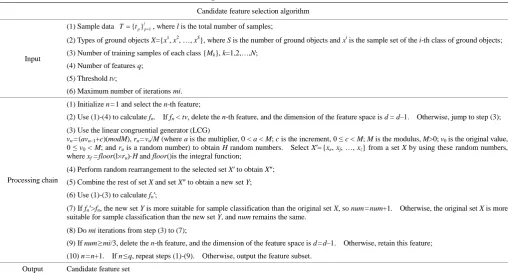
Based on the criterion function fn, the Monte Carlo random
sampling algorithm was used to select the candidate feature subset to reduce the feature dimensionality and to improve the classification efficiency. The processing chain is shown in Table 3.
3.3.2 Removing redundant features that are strongly correlated Because of the possible correlation between some candidate features, the redundant features that are strongly correlated also need to be removed. A correlation coefficient matrix can be built for multiple vectors since the correlation between two variables can be expressed by the correlation coefficient. Therefore, feature parameters with similar classification capabilities can be deleted by analyzing the correlation between these parameters. First, a feature parameter matrix was constructed according to the feature subset that was extracted above. All the features were sorted in ascending order according to fn. Second, the correlation
coefficient between every two columns in the feature parameter matrix was calculated by the nonparametric correlation coefficient, and the correlation coefficient matrix P was obtained:
' ' ' ' 11 1 1 .... : .... : .... n
n n n
r r P r r (6)
Due to the equality of rij and rji, P is a symmetric matrix.
value rij in the correlation coefficient matrix and the threshold T,
the elements Xi and Xj are strongly correlated if rij>T. Thus, the
i-th (or j-th) dimension feature in the feature parameter matrix should be removed to obtain the final optimal feature subset. Table 3 Processing chain for candidate feature set selection
Candidate feature selection algorithm
Input
(1) Sample data { } 1
l p p
T t , where l is the total number of samples;
(2) Types of ground objects X={x1, x2, …, xS}, where S is the number of ground objects and xi is the sample set of the i-th class of ground objects; (3) Number of training samples of each class {Mk}, k=1,2,…,N;
(4) Number of features q; (5) Threshold tv;
(6) Maximum number of iterations mi.
Processing chain
(1) Initialize n=1 and select the n-th feature;
(2) Use (1)-(4) to calculate fn. If fn < tv, delete the n-th feature, and the dimension of the feature space is d = d–1. Otherwise, jump to step (3);
(3) Use the linear congruential generator (LCG)
vu=(avu–1+c)(modM), ru=vu/M (where a is the multiplier, 0 < a < M; c is the increment, 0 ≤ c < M; M is the modulus, M>0; v0 is the original value,
0 ≤ v0 < M; and ru is a random number) to obtain H random numbers. Select X′={xe, xf, …, xz} from a set X by using these random numbers,
where xf =floor(l×ru)·H and floor()is the integral function;
(4) Perform random rearrangement to the selected set X′ to obtain X″; (5) Combine the rest of set X and set X″ to obtain a new set Y; (6) Use (1)-(3) to calculate fn′;
(7) If fn′>fn, the new set Y is more suitable for sample classification than the original set X, so num=num+1. Otherwise, the original set X is more
suitable for sample classification than the new set Y, and num remains the same. (8) Do mi iterations from step (3) to (7);
(9) If num≥mi/3, delete the n-th feature, and the dimension of the feature space is d=d–1. Otherwise, retain this feature; (10) n=n+1. If n≤q, repeat steps (1)-(9). Otherwise, output the feature subset.
Output Candidate feature set
3.4 Object-oriented classification by combining optical and SAR remote sensing images
Support vector machines (SVMs), a universal learning method based on statistic learning theory, have an excellent learning performance and a good generalization ability when solving small-sample, nonlinear and high-dimensional problems. The SVM algorithm was originally used to solve the problem of two-class classification. When the training sample set originates from m (m>2) classes, the set belongs to the multiclass classification problem. At present, many algorithms have extended SVMs to multiclass classification problems, and these algorithms are collectively called multi-category support vector machines (M-SVMs). The one-versus-rest (OVR) method is widely used[61], so this method was utilized to solve the problem of multiclass crop classification in this study. The parameter settings of the SVM model include the type and parameters of the kernel function. Roli F et al.[62] showed that the classification accuracy was generally higher when using a radial basis function (RBF) kernel than when using a polynomial kernel or sigmoid kernel, while using a linear kernel yields the lowest precision. Therefore, the RBF was chosen as the kernel function. With the support of farmland parcels segmented from the optical image as the basic unit for classification, the mean values of multi-features within the farmland parcels were calculated. Because the ranges of the extracted feature parameters were different, the feature parameters were normalized, and then the SVM-OVR classifier was used for classification processing.
4 Results
4.1 Optical-based segmentation of farmland
According to the method in Section 3.1, a mask of the nonfarming areas was built to obtain the range of farmland by using eCognition Developer version 9.0.2. Then, the farmland was resegmented, the segmentation scale was set to range from 10 (very broken) to 80 (very rough) in the interval of 5 and was continuously
adjusted to determine the optimal scale. Then, the shape and compactness parameters were set to 0.3 and 0.6, respectively. These settings focused on the dependence of the spectral information and were closely connected to the crop growth, thereby achieving a better segmentation effect for farmland. The ALV and the corresponding change rate were calculated at different scales, and the change rate threshold of the ALV was set according to the experimental results. After the test, the point that corresponded to the change rate that was less than 0.2 was used to determine the optimal scale. To compare the trends, the change rate of the ALV was increased by a factor of 10 and is shown alongside the ALV in Figure 4. An upward trend was observed in the ALV curve with increasing scale. The fitted curve of the corresponding change rate indicated that the change rate was less than the specified threshold for the first time at a scale of 64. Therefore, the preliminary optimal scale for farmland was 64.
Figure 4 ALV and the corresponding change rate at different segmentation scales
samples from the GF-2 images of the same period, the overlap method[63] was used to calculate the accuracy of the segmentation results. The accuracy evaluation at different scales is shown in Table 4. The extraction accuracy of the farmland parcels initially increased and then decreased with increasing scale, while the number of parcels gradually decreased. The accuracy was the
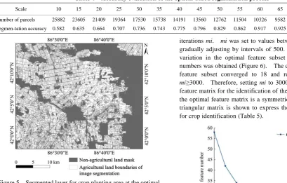
highest (0.925) at a scale of 65, and the number of parcels was relatively small. Therefore, this result was not much different from the predicted best scale of 64, satisfying the optimal segmentation requirement. Through the above process, the complete boundary of the farmland parcels was acquired (Figure 5).
Table 4 Accuracy evaluation of the optical-based segmentation process
Scale 10 15 20 25 30 35 40 45 50 55 60 65 70 75 80
Number of parcels 25882 23605 21409 19364 17530 15738 14191 13560 12762 11504 10326 9582 8970 8351 7889 Segmen-tation accuracy 0.582 0.635 0.664 0.707 0.736 0.743 0.775 0.796 0.829 0.862 0.917 0.925 0.893 0.856 0.821
Figure 5 Segmented layer for crop planting area at the optimal scale
4.2 Feature selection and analysis
4.2.1 Optimal feature subset for crop identification
The WA-BS algorithm was used to determine the optimal feature subset for crop identification from the 58 extracted features through the feature set evaluation criteria. The dimensions of the optimal feature subset and the runtime of the algorithm were controlled by setting the maximum number of
iterations mi. mi was set to values between 0 and 5000 and by gradually adjusting by intervals of 500. Then, the dimensional variation in the optimal feature subset with different iteration numbers was obtained (Figure 6). The dimension of the optimal feature subset converged to 18 and remained constant when mi≥3000. Therefore, setting mi to 3000 could yield an optimal feature matrix for the identification of the 5 crop types. Because the optimal feature matrix is a symmetric matrix, only the lower triangular matrix is shown to express the optimal feature subset for crop identification (Table 5).
Figure 6 Dimensional variation in the optimal feature subsets by the number of iterations
Table 5 Optimal feature matrix for crop classification
Class Wheat Maize Cotton Beets Tomatoes
Wheat
Maize {10,12,25,27,38,41,42,52,57}
Cotton {17,25,31,34,38,42,47,52,53,56,57} {12,25,31,34,38,47,50,56}
Beets {10,17,25,27,31,38,41,43,48,57} {17,31,34,47,50,57} {12,27,34,38,41,43,47,50,52,56,57}
Tomatoes {12,17,25,38,42,48,52,57} {10,17,25,27,31,38,42,47,48,57} {12,17,27,38,41,43,50,52,53,57} {12,27,31,34,43,56} After analyzing the optimal feature matrix, only 18 of the 58
features were involved in the classification of the five crop types, thus greatly reducing the information redundancy and calculations. The feature parameters derived from different polarimetric decompositions greatly contributed to the classification results, mainly originating from Freeman-Vol, Freeman-Dbl, VanZyl-Odd from VanZyl decomposition, two eigenvectors from Cloude decomposition, Yamaguchi-Vol, Yamaguchi-Hlx from Yamaguchi decomposition, Neumann-dela-mod from Neumann decomposition, and A and H from H/A/Alpha decomposition. The scattering properties of the target crops are uncertain and temporally vary, so the scattering echo of each pixel mostly consists of the scattering information of multiple scatterers. Therefore, incoherent target decomposition played a positive role in the classification results.
4.2.2 Optimal feature subset for crop identification
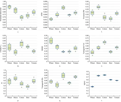
In this section, the optimal features derived from the optical and SAR images during the growing period of various crops were analyzed by boxplots. Figure 7 shows the boxplots of the 18 features in the optimal feature subset, with the 0.5th, 25th, 50th (median), 75th and 99.5th percentiles shown.
As shown in Figure 7, the volume and double-bounce scattering components from Freeman decomposition played a more important role in crop classification than the surface scattering component, and the ability of the volume scattering component to distinguish crop types was greater than that of the double-bounce scattering component. The reason for this finding may be because Freeman decomposition is more accurate at modeling volume scattering, which is influenced by the actual scattering mechanisms of crops. Analyzing the features of volume scattering of various crops from the Freeman decomposition indicated the following: (1) the volume scattering component of cotton during this period was obviously dominant. This period was the growing stage of cotton, and canopy scattering was the main backscattering component. The incident waves scattered many times, so the volume scattering was
increased. (2) Because of the uniform growth of wheat in the ripening stage, the eigenvalue for volume scattering was the smallest among all the crops, and the distribution of the eigenvalues was relatively dispersive. In contrast, the value for double-bounce scattering was large. (3) The eigenvalue for volume scattering of tomatoes was relatively large and its distribution was the most concentrated. The height of beet plants was relatively low, so the reflection of radar waves mainly involved surface reflection. The branches and the ground comprised a pair of orthogonal surfaces, which sometimes caused double-bounce scattering. Therefore, beets had a small eigenvalue of double-bounce scattering. Cloude theory[43] decomposes the polarimetric coherence matrix into a weighted sum of three components, and each component corresponds to a scattering mechanism (single scattering, bidirectional scattering and cross scattering). Therefore, Cloude decomposition can include all the scattering mechanisms. Analyzing the different boxplot values ofthe two-component Cloude-T11 and Cloude-T33
features indicated that the two components of Cloude decomposition exhibited a strong ability to describe ground objects with different scattering mechanisms.
a. b. c.
d. e. f.
j. k. l.
m. n. o.
p. q. r.
Figure 7 Boxplots of the optimal feature subset. (a-r) are the optimal features extracted from the 58 features The scattering entropy H reflects the randomness degree
between isotropic scattering (H=0) and completely random scattering (H=1) of a scattering medium. The larger the value of H is, the higher the randomness degree. When analyzing the scattering entropy of various crops, the scattering type of maize during this period was complicated. Here, maize was in the early harvest stage, so the maize canopy was dense, resulting in a high scattering entropy. In contrast, beets were in the middle of the growing period, and the row spacing of beets was relatively large when seeding, so the area of bare soil was large and the surface structure was simple. In this case, the target contained relatively simple scatters, and the polarimetric entropy was relatively low. The anti-entropy A, a supplementary parameter of the scattering entropy H, is also in the optimal feature set for crop identification. The energy parameter SPAN contains the intensity information of the scattering mechanism, so introducing SPAN into the classification helped to distinguish ground objects with the same scattering mechanism but with different scattering intensities. The RVI can reflect the vegetation features and volume scattering information, which exhibited certain differences because the density of crop covers during this period was different. The density of wheat at harvest was the highest, so the incident waves had sufficient random scattering in the medium, resulting in the
depolarization of the scattering echo. The planting of beets was sparse, and the vegetation structure was relatively simple, so any random scattering occurring when the incident waves interacted with the vegetation was rare. Most of the incident waves directly escaped after single- or double-bounce scattering, and the depolarization effect was low. In addition, DERD can be used to compare the importance of different scattering mechanisms, which played a certain auxiliary role in crop classification. The SE is defined based on the intensity and polarization; the intensity contribution is related to the backscattering energy, and the polarization contribution is related to the polarizability. Analyzing the SE boxplot, the value of maize was the largest during this period, and the SEs of tomatoes, wheat, cotton, and sugar beets were lower, indirectly reflecting differences in the backscattering energy of various crops.
uniform, and the texture was fine; the ASM and CON values of wheat were the lowest. The NDVI has an important ecological significance and can reflect the crop growth information, so it was included in the optimal feature set for crop identification. However, due to the similar NDVI values for cotton and maize during this period, the NDVI had a weaker ability to distinguish between the two crops, so it was not the main feature to separate cotton and maize.
4.3 Crop classification and accuracy assessment
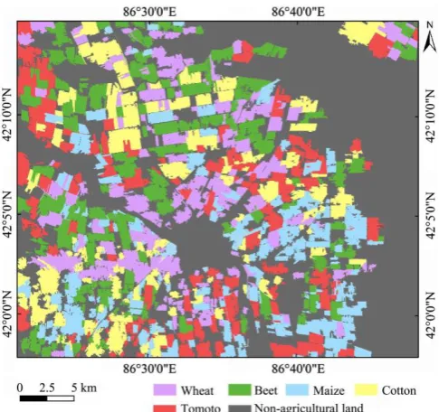
With the SVM-OVR classifier, referred to in Section 3.4, the training samples of the five types of crops were used to train the model, and the validation samples were used for accuracy assessment. When employing the classifier, the kernel parameter γand the penalty factor C in the RBF kernel need to be determined. A cross-validation algorithm was employed to determine these two parameters[64]. In this study, the cross-validation parameter selection model from LIBSVM-3.22 was used to search for the optimal set of γ and C. After the experiment, the optimal parameters were considered γ=0.125 and C=512. Finally, with the optimal feature subset, the classifier was employed in object-oriented classification. The crop classification result is shown in Figure 8, and the statistics of the crop acreage were calculated using ArcGIS 10.3 (Figure 9). From Figure 8, crop-type mapping supported by segmentation from the optical image accurately identified crops and avoided the “salt-and-pepper” phenomenon that often appears in pixel-based classification. The crop type of each parcel was indicated, and confusion among different crop types was rare. Analyzing Figure 9, tomatoes were the most widely planted crop in the region, with an area of 156.5 km2, accounting for 25.98% of the total planting area, followed by cotton (147.6 km2, accounting for 24.51%),
wheat (112.4 km2, accounting for 18.66%), beets (97.5 km2, accounting for 16.19%) and maize (88.3 km2, accounting for 14.66%). According to the data published in the 2018 Xinjiang Agricultural Statistical Yearbook, the actual planting areas of tomatoes, cotton, wheat, beet and maize in the study area were 165.2 km2, 151.8 km2, 107.3 km2, 100.7 km2 and 82.6 km2 respectively. Therefore, the feasibility and effectiveness of this method have been proved by the experiment.
Figure 8 Crop classification result derived from multifeatures and optical-based segmentation
Figure 9 Crop planting area of the five crops
The accuracy of the crop classification results was evaluated with the validation samples to assess the effect of the crop identification model. A confusion matrix, a standard format for accuracy evaluation, was used to calculate the overall accuracy (OA), the user’s accuracy (UA), the producer’s accuracy (PA), and the Kappa coefficient. According to the confusion matrix[65] (Table 6), the OA of the five crop types was 89.50%, and the Kappa coefficient was 0.87. Therefore, the proposed method achieved a good performance, indicating that the model has strong practicability for identifying crop types. Generally, when the PA and UA are both higher than 85%, the crop classification is considered to be reliable[66]. Therefore, the results showed that the extracted features from the optical and full polarimetric SAR images with the support of farmland parcels can be used for crop-type mapping, satisfying the effect of crop identification.
Table 6 Classification accuracy of the proposed method
Class Wheat (parcel)
Maize (parcel)
Cotton (parcel)
Beets (parcel)
Tomatoes (parcel) UA/%
Wheat (parcel) 225 4 13 0 2 87.55
Maize (parcel) 0 221 3 10 0 90.20
Cotton (parcel) 5 9 235 12 17 86.72
Beets (parcel) 12 0 0 301 14 96.47
Tomatoes (parcel) 9 16 17 6 288 86.23
PA/% 89.64 88.40 87.69 91.49 89.72 OA 89.50% Kappa coefficient 0.87
5 Discussion
5.1 Comparison with different datasets
detail of the image, which led to confusion between crop types and other classes. Because a high variability resulting from the backscattering effect of ground objects on radar beams exists within a class, SAR image segmentation divided a homogenous region into several parcels. In the process of farmland extraction, some fields were classified as non-agricultural land and thus masked, resulting in an omission error. For example, the UAs and PAs of wheat and maize were not ideal with large commission and omission errors, declining from 76.89% to 74.39% for wheat and from 75.48% to 78.17% for maize. However, the classification results were improved by the object-oriented classification based on optical image segmentation, which was more suitable to extract farmland parcels and reduced salt-and-pepper noise. From the above comparison, the proposed method is better for crop classification, helping to improve classification accuracy.
Table 7 Classification accuracy of the comparative experiment
Class Wheat (parcel)
Maize (parcel)
Cotton (parcel)
Beets (parcel)
Tomatoes (parcel) UA/%
Wheat (parcel) 183 15 0 13 27 76.89
Maize (parcel) 30 197 12 8 14 75.48
Cotton (parcel) 9 16 242 6 9 85.82
Beets (parcel) 13 19 23 270 0 83.08
Tomatoes (parcel) 11 5 3 19 275 87.86
PA/% 74.39 78.17 86.43 85.44 84.62 OA 82.24% Kappa coefficient 0.78
Figure 10 Crop classification results derived from multifeatures and SAR-based segmentation
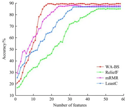
5.2 Comparison with different feature selection methods To verify the performance of WA-BS, a comparison between the proposed method and three baseline methods (ReliefF[58], mRMR[59] and LeastC[67]) was performed on a 3.4 GHz, 64 bit AMD CPU. The above comparison models are filter models and are independent of classifiers. The overall accuracy of crop classification conducted by the SVM classifier with the same parameter settings is shown in Figure 11. The accuracy of crop classification using the optimal feature subset achieved by the WA-BS algorithm is 89.50%, which is better than that of other feature selection methods. The mRMR algorithm considers the relevance between features and identifying targets as well as the
independence between features and achieved a classification accuracy of 87.59%. The LeastC algorithm is fault-tolerant to noise and is not affected by feature interaction; the classification accuracy using the optimal features achieved by the LeastC algorithm is 86.74%. However, the ReliefF algorithm cannot effectively remove redundant features due to the lack of consideration of the correlation between features, reaching a crop classification accuracy of only 85.01%. The dimensions of the optimal features obtained using WA-BS, ReliefF, mRMR and LeastC algorithms are 18, 46, 25 and 33, respectively. Therefore, the WA-BS algorithm can effectively remove redundant features that are strongly correlated and achieves a higher classification accuracy via the optimal feature subset.
Figure 11 Overall accuracy using the optimal feature subset obtained by different feature selection methods
6 Conclusions
Crop-type mapping with a single type of remote sensing image sometimes has unsatisfactory precision. The purpose of this study is to promote the collaborative application of optical and SAR remote sensing data in agriculture. A framework for crop identification is proposed based on GF-2 and GF-3 images. A demonstration in Xinjiang Uygur Autonomous Region targeting wheat, maize, cotton, beet and tomato crops showed that the crop growth features derived from the GF-2 and GF-3 images within farmland parcels segmented from an optical image can achieve good classification results, with an overall accuracy of 89.50%, which is better than the accuracy of 82.24% derived from SAR-based segmentation. Compared with the ReliefF, mRMR and LeastC feature selection algorithms, the WA-BS algorithm proposed in this paper can effectively remove redundant features that are strongly correlated and can achieve a higher classification accuracy via the obtained optimal feature subset. The results indicate that the combination of optical and full polarimetric SAR images under the constraints of farmland parcels can be used for crop-type mapping, resulting in crop identification. Furthermore, this study extends the application of the GF series satellites to agriculture and indicates their great potential in crop monitoring.
Acknowledgements
61375002). Our sincere thanks go to the students at the State Key Laboratory of Remote Sensing Science for their assistance during the field survey campaigns.
[References]
[1] Mokhtari A, Noory H, Vazifedoust M. Improving crop yield estimation by assimilating LAI and inputting satellite-based surface incoming solar radiation into SWAP model. Agricultural and Forest Meteorology, 2018; 250: 159–170.
[2] Gallego F J, Kussul N, Skakun S, Kravchenko O, Shelestov A, Kussul O. Efficiency assessment of using satellite data for crop area estimation in Ukraine. International Journal of Applied Earth Observation and Geoinformation, 2014; 29: 22–30.
[3] Chen Y L, Song X D, Wang S S, Huang J F, Mansaray L R. Impacts of spatial heterogeneity on crop area mapping in Canada using MODIS data. ISPRS Journal of Photogrammetry and Remote Sensing, 2016; 119: 451–461.
[4] He Y H Z, Wang C L, Chen F, Jia H C, Liang D, Yang A Q. Feature comparison and optimization for 30-m winter wheat mapping based on Landsat-8 and Sentinel-2 data using random forest algorithm. Remote Sensing, 2019:11(5): 535.
[5] Asgarian A, Soffianian A, Pourmanafi S. Crop type mapping in a highly fragmented and heterogeneous agricultural landscape: A case of central Iran using multi-temporal Landsat 8 imagery. Computers and Electronics in Agriculture, 2016; 127: 531–540.
[6] Lessel J, Ceccato P. Creating a basic customizable framework for crop detection using Landsat imagery. International Journal of Remote Sensing, 2016; 37(24): 6097–6107.
[7] Clauss K, Ottinger M, Leinenkugel P, Kuenzer C. Estimating rice production in the Mekong Delta, Vietnam, utilizing time series of Sentinel-1 SAR data. International Journal of Applied Earth Observation and Geoinformation, 2018; 73: 574–585.
[8] Guo J, Wei P L, Liu J, Jin B, Su B F, Zhou Z S. Crop Classification based on differential characteristics of H/alpha scattering parameters for multitemporal quad- and dual-polarization SAR images. IEEE Transactions on Geoscience and Remote Sensing, 2018; 56(10): 6111–6123.
[9] Panigrahy S, Jain V, Patnaik C, Parihar J S. Identification of Aman rice crop in Bangladesh using temporal C-band SAR - a feasibility study. Journal of the Indian Society of Remote Sensing, 2012; 40 (4): 599–606. [10] Saich P, Borgeaud M. Interpreting ERS SAR signatures of agricultural
crops in Flevoland, 1993-1996. IEEE Transactions on Geoscience and Remote Sensing, 2000; 38(2): 651–657.
[11] Hong G, Wang S S, Li J H, Huang J F. Fully polarimetric Synthetic Aperture Radar (SAR) processing for crop type identification. Photogrammetric Engineering and Remote Sensing, 2015; 81(2): 109–117. [12] Silva W F, Rudorff B F T, Formaggio A R, Paradella W R, Mura J C,
Simulated multipolarized MAPSAR images to distinguish agricultural crops. Scientia Agricola, 2012; 69(3): 201–209.
[13] Li H P, Zhang C, Zhang S Q, Atkinson P M. Full year crop monitoring and separability assessment with fully-polarimetric L-band UAVSAR: A case study in the Sacramento Valley, California. International Journal of Applied Earth Observation and Geoinformation, 2019; 74: 45–56. [14] McNairn H, Champagne C, Shang J, Holmstrom D, Reichert G.
Integration of optical and Synthetic Aperture Radar (SAR) imagery for delivering operational annual crop inventories. ISPRS Journal of Photogrammetry and Remote Sensing, 2009; 64(5): 434–449.
[15] Yang H, Yang G J, Gaulton R, Zhao C J, Li Z H, Taylor J, et al. In-season biomass estimation of oilseed rape (Brassica napus L.) using fully polarimetric SAR imagery. Precision Agriculture, 2019; 20(3): 630–648.
[16] Uppala D, Kothapalli R V, Poloju S, Mullapudi S, Dadhwal V K. Rice Crop discrimination using single date RISAT1 hybrid (RH, RV) polarimetric data. Photogrammetric Engineering and Remote Sensing, 2015; 81(7): 557–563.
[17] Cable J W, Kovacs J M, Jiao X F, Shang J L. Agricultural monitoring in northeastern Ontario, Canada, using multi-temporal polarimetric RADARSAT-2 data. Remote Sensing, 2014; 6(3): 2343–2371.
[18] Engelbrecht J, Kemp J, Inggs M. The phenology of an agricultural region as expressed by polarimetric decomposition and vegetation indices. In 2013 IEEE International Geoscience and Remote Sensing Symposium, 2013; pp.3339–3342.
[19] Haldar D, Patnaik C. Synergistic use of multi-temporal Radarsat SAR and AWiFS data for Rabi rice identification. Journal of the Indian Society of Remote Sensing, 2010; 38(1): 153–160.
[20] Jiao X F, Kovacs J M, Shang J L, McNairn H, Walters D, Ma B L, et al. Object-oriented crop mapping and monitoring using multi-temporal polarimetric RADARSAT-2 data. ISPRS Journal of Photogrammetry and Remote Sensing, 2014; 96: 38–46.
[21] Forkuor G, Conrad C, Thiel M, Ullmann T, Zoungrana E. Integration of optical and Synthetic Aperture Radar imagery for improving crop mapping in northwestern Benin, west Africa. Remote Sensing, 2014; 6(7): 6472–6499.
[22] Ameline M, Fieuzal R, Betbeder J, Berthoumieu J F, Baup F. Estimation of corn yield by assimilating SAR and optical time series into a simplified agro-meteorological Model: from diagnostic to forecast. IEEE Journal of Selected Topics in Applied Earth Observations and Remote Sensing, 2018; 11(12): 4747–4760.
[23] Lu L Z, Tao Y, Di L P. Object-based plastic-mulched landcover extraction using integrated Sentinel-1 and Sentinel-2 data. Remote Sensing, 2018; 10(11): 1820.
[24] Steinhausen M J, Wagner P D, Narasimhan B, Waske B. Combining Sentinel-1 and Sentinel-2 data for improved land use and land cover mapping of monsoon regions. International Journal of Applied Earth Observation and Geoinformation, 2018; 73: 595–604.
[25] De Alban J D T, Connette G M, Oswald P, Webb E L. Combined Landsat and L-band SAR data improves land cover classification and change detection in dynamic tropical landscapes. Remote Sensing, 2018; 10(2): 306
[26] Zhang J X, Yang J H, Zhao Z, Li H T, Zhang Y H. Block-regression based fusion of optical and SAR imagery for feature enhancement. International Journal of Remote Sensing, 2010; 31(9): 2325–2345. [27] Hong G, Zhang Y, Mercer B. A wavelet and IHS integration method to
fuse high resolution SAR with moderate resolution multispectral images. Photogrammetric Engineering and Remote Sensing, 2009; 75(10): 1213–1223.
[28] Rajah P, Odindi J, Mutanga O. Feature level image fusion of optical imagery and Synthetic Aperture Radar (SAR) for invasive alien plant species detection and mapping. Remote Sensing Applications: Society and Environment, 2018; 10: 198–208.
[29] Deledalle C A, Denis L, Tabti S, Tupin F. MuLoG, or how to apply Gaussian denoisers to multi-channel SAR speckle reduction? IEEE Transactions on Image Processing, 2017; 26(9): 4389–4403.
[30] Prudente V H R, da Silva B B, Johann J A, Mercante E, Oldoni L V. Comparative assessment between per-pixel and object-oriented for mapping land cover and use. Engenharia Agricola, 2017; 37(5): 1015–1027. [31] Frery A C, Correia A H, Freitas C D. Classifying multifrequency fully polarimetric imagery with multiple sources of statistical evidence and contextual information. IEEE Transactions on Geoscience and Remote Sensing, 2007; 45(10): 3098–3109.
[32] Boudaren M E Y, An L, Pieczynski W. Unsupervised segmentation of SAR images using Gaussian mixture-hidden evidential Markov fields. IEEE Geoscience and Remote Sensing Letters, 2016; 13(12): 1865–1869. [33] Huang S Q, Huang W Z, Zhang T. A new SAR image segmentation
algorithm for the detection of target and shadow regions. Scientific Reports, 2016, 6.
[34] Wu Q, Zhong R F, Zhao W J, Song K, Du L M. Land-cover classification using GF-2 images and airborne Lidar data based on Random Forest. International Journal of Remote Sensing, 2019; 40(5-6): 2410–2426. [35] Zhang M M, Chen F, Tian B S. Glacial lake detection from GaoFen-2
multispectral imagery using an integrated nonlocal active contour approach: a case study of the Altai Mountains, northern Xinjiang province. Water, 2018; 10(4): 455.
[36] Wang Z H, Yang X M, Liu Y M, Lu C. Extraction of coastal raft cultivation area with heterogeneous water background by thresholding object-based visually salient NDVI from high spatial resolution imagery. Remote Sensing Letters, 2018; 9(9): 839–846.
[37] Vermote E F, Tanre D, Deuze J L, Herman M, Morcrette J J. Second simulation of the satellite signal in the solar spectrum, 6S: an overview. Ieee Transactions on Geoscience and Remote Sensing, 1997; 35(3): 675–686.
[39] McCoy R M. Field methods in remote sensing; Guilford Press: New York City, NY, USA, 2005.
[40] Woodcock C E, Strahler A H. The factor of scale in remote-sensing. Remote Sensing of Environment, 1987; 21(3): 311–332.
[41] Woodcock C E, Strahler A H, Jupp D L B. The use of variograms in remote sensing: I. Scene models and simulated images. Remote Sensing of Environment, 1988; 25(3): 323–348.
[42] Canisius F, Shang J L, Liu J G, Huang X D, Ma B L, Jiao X F, et al. Tracking crop phenological development using multi-temporal polarimetric Radarsat-2 data. Remote Sensing of Environment, 2018; 210: 508–518. [43] Cloude S R, Pottier E. A review of target decomposition theorems in
radar polarimetry. IEEE Transactions on Geoscience and Remote Sensing, 1996; 34(2): 498–518.
[44] Freeman A, Durden S L. A three-component scattering model for polarimetric SAR data. IEEE Transactions on Geoscience and Remote Sensing, 1998; 36(3): 963–973
[45] Vanzyl J J. Application of Cloude's target decomposition theorem to polarimetric imaging radar data. Proc. SPIE, 1993; 184: 184–191. [46] Krogager E. New decomposition of the radar target scattering matrix.
Electronics Letters, 1990; 26(18): 1525–1527.
[47] Lee J S, Pottier E. Polarimetric radar imaging from basics to applications. Boca Raton: CRC Press Taylor and Francis Group, 2009; pp.214–215. [48] Barnes R M. Roll-invariant decompositions for the polarization
covariance matrix. In Proceedings of Polarimetry Technology Workshop, Huntsville, AL, 1998; pp.371–389.
[49] Holm W A, Barnes R M. On radar polarization mixed target state decomposition techniques. In Proceedings of the IEEE National Radar Conference, Ann Arbor, MI, USA, 20–21 April 1988; pp.249–254. [50] Yamaguchi Y, Moriyama T, Ishido M, Yamada H. Four-component
scattering model for polarimetric SAR image decomposition. IEEE Transactions on Geoscience and Remote Sensing, 2005; 43(8): 1699–1706. [51] Huynen J R. Phenomenological theory of radar targets. PhD
Dissertation, Tech. Univ. Delft, Delft, The Netherlands, 1970.
[52] Neumann M, Ferro-Famil L, Pottier E. A general model based polarimetric decomposition scheme for vegetated areas. In Proceedings of the 4th International Workshop on Science and Applications of SAR Polarimetry and Polarimetric Interferometry (ESRIN), Frascati, Italy, 26–30 January, 2009.
[53] Cloude S R, Pottier E. An entropy based classification scheme for land applications of polarimetric SAR. IEEE Transactions on Geoscience and Remote Sensing, 1997; 35(1): 68–78.
[54] Shaban M A, Dikshit O. Improvement of classification in urban areas by
the use of textural features: the case study of Lucknow city, Uttar Pradesh International Journal of Remote Sensing, 2001; 22(4): 565–593.
[55] Feldens P. Sensitivity of texture parameters to acoustic incidence angle in multibeam backscatter. Ieee Geoscience and Remote Sensing Letters, 2017; 14(12): 2215–2219.
[56] Li C R, Guan X Y, Yang P H, Huang Y Y, Huang W, Chen H F. CDF space covariance matrix of Gabor wavelet with convolutional neural network for texture recognition. IEEE Access, 2019; 7: 30693–30701. [57] Chen M, Strobl J. Multispectral textured image segmentation using a
multi-resolution fuzzy Markov random field model on variable scales in the wavelet domain. International Journal of Remote Sensing, 2013; 34(13): 4550–4569.
[58] Robnik-Šikonja M, Kononenko I. Theoretical and empirical analysis of Relief F and RRelief F. Machine Learning, 2003; 53(1): 23–69. [59] Peng H C, Long F H, Ding C. Feature selection based on mutual
information: Criteria of max-dependency, max-relevance, and min-redundancy. IEEE Transactions on Pattern Analysis and Machine Intelligence, 2005; 27(8): 1226–1238.
[60] Chen X, Gu Y F. Class-specific feature selection with local geometric structure and discriminative information based on sparse similar samples. Ieee Geoscience and Remote Sensing Letters, 2015; 12(7): 1392–1396. [61] Kim K J, Ahn H. A corporate credit rating model using multi-class
support vector machines with an ordinal pairwise partitioning approach. Computers & Operations Research, 2012; 39(8): 1800–1811.
[62] Roli F, Fumera G. Support vector machines for remote-sensing image classification. In Image and Signal Processing for Remote Sensing Vi, Serpico S B, Ed. 2001; Vol. 4170, pp.160–166.
[63] Moller M, Lymburner L, Volk M. The comparison index: A tool for assessing the accuracy of image segmentation. International Journal of Applied Earth Observation and Geoinformation, 2007; 9(3): 311–321. [64] Keerthi S S, Lin C J. Asymptotic behaviors of support vector machines
with Gaussian kernel. Neural Computation, 2003; 15(7): 1667–1689. [65] Congalton R G. Accuracy assessment and validation of remotely sensed
and other spatial information. International Journal of Wildland Fire, 2001; 10(3-4): 321–328.
[66] Skakun S, Kussul N, Shelestov A Y, Lavreniuk M, Kussul O. Efficiency assessment of multitemporal C-band Radarsat-2 intensity and Landsat-8 surface reflectance satellite imagery for crop classification in Ukraine. IEEE Journal of Selected Topics in Applied Earth Observations and Remote Sensing, 2016; 9(8): 3712–3719.