Reexamination of Whether Accrual Quality Is a Price Factor
May Xiaoyan Bao1, Xiaoyan Cheng2, John Geppert3 & David B. Smith3 1
Peter T. Paul College of Business and Economics, University of New Hampshire, USA 2 College of Business Administration, University of Nebraska-Omaha, USA
3
College of Business, University of Nebraska-Lincoln, USA
Correspondence: May Xiaoyan Bao Peter T. Paul College of Business and Economics, University of New Hampshire, 10 Garrison Ave, Durham, NH, 03824, USA
Received: June 13, 2019 Accepted: July 5, 2019 Online Published: July 8, 2019
doi:10.5430/afr.v8n3p103 URL: https://doi.org/10.5430/afr.v8n3p103
Abstract
In this study, we investigate whether accrual quality is a factor in capital asset pricing. Our analysis consists of two parts. First, we use a panel data regression that controls for cross-section fixed effects to implement the second stage of the Fama-MacBeth regression (Petersen 2009). In the second part, we use the Campbell (1991) return decomposition and vector autoregressive model (VAR) to decompose the two-stage cross-sectional regressions. This allows us to investigate whether accrual quality is a priced factor in terms of the three components of the return, which include one-period expected return, cash flow news and discount-rate news.
Keywords: asset-pricing tests, accruals quality, information risk, portfolio theory and diversification, return decomposition
We thank the financial support of Peter T. Paul Financial Policy Center at Peter T. Paul College of Business and Economics, University of New Hampshire.
1. Introduction
Whether information risk impacts a firm’s cost of equity capital has been a controversial issue in the accounting and finance literature. Prior theoretical research shows that information risk is a non-diversifiable risk factor (e.g., Amihud & Mendelson, 1986; Easley & O’Hara, 2004; Leuz & Verrecchia, 2005; Francis, LaFond, Olsson, & Schipper, 2005). This research conflicts with empirical findings that suggest the information quality risk is diversifiable in the portfolios of many assets. In the accounting empirical literature, accrual quality is a proxy for information quality risk and is measured with the augmented Dechow & Dichev (2002) method. This stream of empirical research suggests that the accrual quality factor may not be priced in the excess return along with the Fama and French three factors in the conventional Fama-MacBeth two-pass asset pricing test (Core, Guay, & Verdi, 2008; Ogneva, 2012; Kim & Qi, 2010). As the link between information quality and the cost of capital is one of the most fundamental doctrines in finance and accounting (Leuz & Verrecchia, 2005), a further investigation is warranted. In our study, we investigate whether accrual quality is a priced factor to better understand the conflicts between the theoretical research and prior empirical evidence.
We take two approaches. First, we reexamine the issue, using a different econometric technique from those used in previous accounting and finance studies to implement the Fama- MacBeth two-pass pricing. We control firm-fixed effect in the Fama-MacBeth two-passing pricing model which uses panel datasets (e.g. data sets that contain observations on multiple firms in multiple years) as suggested by Petersen (2009) to correct biased Fama- Macbeth standard errors. (Note 1) Second, we examine whether accrual quality is priced in components of a firm’s return. We use a linear approximate framework developed by Campbell & Shiller (1988a) to decompose the realized stock return into three components: the one-period expected stock return{𝐸𝑡−1[𝑟𝑡]}, the cash-flow news (𝑁𝑐𝑓,𝑡) , and the
negative expected –return news (−𝑁𝑟,𝑡). The decomposed returns provide insights into why accrual quality is a
Our first exploration (that reconsiders prior implemented econometric techniques) is motivated by evidence provided in Petersen (2009). His research identifies inconsistencies in the application of the Fama-MacBeth approach in the finance literature. He suggests that the Fama-MacBeth standard errors calculated in prior empirical studies may be biased in the panel datasets so that the magnitude of the bias is a function of the serial correlation of both the independent variable and the residual within a cluster and the number of time periods per firm (or cluster) (Petersen, 2009). Failing to control for firm fixed effects in the panel datasets is a contributor to the biased standard errors. We motivate the second examination to understand why and how information quality affects the firms’ cost of capital. Leuz & Verrechia (2005) show that information quality affects the firms’ cost of capital through the association between information quality and firms’ expected cash flow. Leuz & Verrechia (2005) model a setting in which reporting quality affects investment choice, which in turn impacts the expected cash flow of firms. And the expected cash flow of firms in turn reduces the firms’ cost of capital.
We suggest that information risk’s impact may be explained by the decomposed return’s effects on cash-flow news and discount news. The news about cash flows is more related to firm fundamentals than other return components because of its link to production. The accuracy of managements’ estimates related to production capability and impact of firms’ information quality on firms’ investment choices influences investors’ perception of the firm’s fundamentals so that investors price misalignment risk generated from poor reporting in the firms’ cost of capital. This contrasts with the news about discount rates, which can reflect time-varying risk aversion or investor sentiment. The market price of risk decreases if investors are less risk aversion (Leuz & Verrechia, 2005). In other words, the firms’ cost of capital reduces when the risk tolerance of the market increases. High accrual quality reflects the managements’ ability and incentive to estimate earnings in a reliable and timely way. Management opportunism affects its’ estimates associated with firm production and risk aversion activities, reducing accrual quality and influencing investors’ demands related to the risk premium for their investments in the firm.
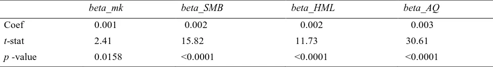
Our findings suggest that accrual quality is a non-diversifiable risk premium factor. Our findings support the prediction of the theoretical model of Luez & Verrechia (2005) that idiosyncratic differences in information quality are priced in the cost of capital in equilibrium through the association between information quality and expected cash flow without a proportional increase in the covariance of these cash flows with the market. The association between information quality and expected cash flows is linked with the association between information quality and firms’ fundamentals. First, our results show that the coefficient on the accrual quality factor (AQ_factor) in the second stage of the Fama-MacBeth two- stage regression, when implemented with cross-sectional fixed effects, is significant and equal to 0.003 (t- stat 30.61 and p-value <0.0001) to the sample period from April 1971 to March 2002, a total of 21,681 firms. The positive coefficient suggests that investors demand a higher risk premium from firms with higher information quality risk.
In the second part of our analysis, we investigate whether accrual quality is a priced factor in asset returns that are decomposed into three components: one-period expected returns, negative news about discount rates and news about cash flows (Campbell & Shiller, 1988a; Campbell, 1991). Results from decomposition of market returns show that the accrual quality factor is priced in the cash flow news component. The coefficients (t- stat and p- value) on the AQ_factor related to the cash flow news, the negative discount news, and the one-period expected return are equal to 0.004 (34.05 and <0.0001), -0.0004 (-33.85 and <0.0001), and -0.0003 (-26.66 and <0.0001), respectively. The negative coefficients on negative news about discount rates and the one-period expected return indicates that the accrual quality is not the priced premium for the component of negative news about discount rates and the component of one-period expected return. (Note 3) As predicted by Leuz & Verrechia (2005), the firms’ cost of capital reduces with the increase of expected cash flow and the decrease of the investors’ risk aversion. The findings that information quality is priced at the firms’ cost of capital is driven by that information quality is priced in cash flow news component of firms’ cost of equity capital. The association between firms’ information quality and firms’ expected cash flow explains the direct link between information quality and cost of capital that does not rely on liquidity or shareholder base effects (Leuz & Verrechia, 2005).
support the prediction of the theoretical model that information quality is priced at a firms’ cost of capital through the real effects of information quality on firms’ capital allocation choice, which in turn affects the level of expected cash flows of firms. The expected cash flows in turn positively affect the firms’ cost of capital as analyzed in Leuz &Verrecchia (2005). Overall, our study reconciles the conflicts between theoretical research and empirical research in the direct link between information quality risk and a firm’s cost of equity capital without relying on liquidity which is explained by information asymmetry or shareholder base effects.
The remainder of the paper proceeds as follows. In the next section, we discuss the literature and the development of the research questions. Section 3 describes our sample and data. Section 4 presents our methodology, including the measurement of the accrual quality, implemented two-stage regressions, and decomposition framework, and the results. Section 5 provides additional tests. Section 6 concludes the paper.
2. Literature Review and Development of Research Questions
2.1 Review of Literature Investigating Price of Accrual Quality
Whether accrual quality is priced in the excess return as a price-risk factor remains controversial in the accounting and finance literature. Theoretical research suggests that information quality and firms’ cost of capital are linked either directly or indirectly via market liquidity. Leuz & Verrecchia (2005) build a model to capture the direct link between information quality and firms’ cost of capital through the real effect of information quality. In their model information quality affects firms’ future cash flows, not just the perceptions of these cash flows of market participants. According to the model, information quality can affect firms’ capital allocation choices; investment choices can affect firms’ expected cash flows without a proportional increase in the covariance of these cash flows to the market; and hence, firms’ cost of capital decreases (increase) with information quality (information quality risk). Their model reveals that the effect on the firms’ cost of capital depends on how fast prices increase relative to the expected cash flow, which is associated with information quality through investment alignment. Cost of capital falls if the market equilibrium price of those cash flows rises faster than the expected cash flows. Amihud & Mendelson (1986) illustrate an indirect link between information quality and firms’ expected returns by analyzing a liquidity-based model in which expected returns increase in the spread (or the amount of information asymmetry). Easley & O’Hara (2004) model that investors demand a lower return for stocks with greater public and less private information. Easley, Hvidkjaer, & O’Hara (2010) find that the PIN factor highlights that information risk is a factor in asset pricing. Kravet & Shevlin (2010) use accrual quality to capture the information risk and the discretionary component of accrual quality to capture discretionary information risk. They find an increase in the pricing of discretionary information risk after restatement announcements, indicating that investors demand a risk premium for bearing information risk. Armstrong, Core, Taylor, & Verrecchia (2011) find that information asymmetry is positively related to the firms’ cost of capital when the degree of market competition is low.
Francis, LaFond, Olsson, & Schipper (FLOS, 2005 hereafter) make one of first attempts to examine whether the accrual quality (AQ) is a determinant of the cost of capital. FLOS find that poorer AQ is associated with larger costs of debt and equity. Core, Guay, & Verdi (CGV, 2008 hereafter) argue that FLOS base their inference, in part, on coefficients from time-series regressions of contemporaneous stock returns to portfolios that mimic exposure to AQ, the market, size, and book-to-market. CGV (2008) notes that FLOS (2005) only conduct the first pass of conventional asset pricing tests (e.g. Fama & MacBeth 1973) and also argue that FLOS’ time-series regressions of contemporaneous stock returns on contemporaneous factor returns do not test the hypothesis that AQ is a priced risk factor. CGV (2008) then conducts both the first and second pass regression tests and find no evidence that AQ is a priced risk factor.
empirical research suggests that information quality risk is a type of idiosyncratic risk and can be diversified or embodied in HML and/or SMB.
2.2 Development of Research Questions
Petersen (2009) has provided evidence about inconsistencies in the application of the Fama-MacBeth approach in the finance literature. He suggests that the Fama-MacBeth standard errors calculated in prior empirical studies might be biased so that the magnitude of the bias is a function of the serial correlation of both the independent variable and the residual within a cluster and the number of time periods per firm (or cluster) (Petersen, 2009). Since the Fama-MacBeth procedure is designed to address a time effect, the time effect need not be controlled in the Fama-MacBeth procedure (Petersen, 2009). However, increases in the firming effect actually reduce the estimated Fama-MacBeth standard error at the same time it increases the true standard error of the estimated coefficients (Petersen, 2009).
In our study, we focus on Petersen (2009)’s framework. Petersen (2009) evaluates the appropriate econometric approach for panel data sets which contain observations on multiple firms in multiple years. Petersen (2009) states “although the literature has used an assortment of methods to estimate standard errors in panel data sets, the chosen method is often incorrect…..only twenty-nine percent of the papers which use the Fama-MacBeth procedure included dummy variables to control for fixed effects”. To demonstrate how the different methods for estimating standard errors compares, Petersen (2009) uses a dataset from Daniel and Titman (2006) as a real world asset price application. The discussions based on this dataset in Petersen (2009) justify our study. Similar to the analysis, we use the equity return regressions with a monthly equity return as the dependent variable (left hand side of the regression). Similar to the independent variables in the example of Daniel & Titman (2006) (e.g. lagged book-to-market ratio, historic changes in the book and market values, and a measure of the firm’s equity issuance), betas of the factors as independent variables, which are obtained from the first pass of the Fama-MacBeth two pass procedure in our study, are persistent. The persistence of betas can be controlled by adding firm dummies in the regression. The addition of firm dummies to a regression is the procedure to control for firm fixed effects. Petersen (2009) compares coefficient and standard error estimates of the equity return regressions of datasets from Daniel & Titman (2006) among OLS coefficients with white standard errors, with time (month) dummies, and the Fama-MacBeth (in table 6 of Petersen (2009)). Petersen (2009) reports that the Fama-MacBeth standard errors perform better in the presence of a time effect than a firm effect. Given the Fama-MacBeth approach was designed to deal with time effects in a panel data set, not firm effects, the Fama-MacBeth standard errors are biased in the presence of a firm effect (Petersen, 2009). To control for firm fixed effects, we regress firm specific excess returns on the betas of the factors obtained from the first pass of Fama-MacBeth procedure with firm fixed effects, denoted “C”. The assumption is that “C” is constant over time. “C” contains unobserved firm characteristics—such as managerial quality or structure—that can be viewed as being (rough) constant over the period (Wooldridge, 2001).
In addition, Petersen (2009) assumes temporary firm fixed effects in his simulated data. For example, the firm effect is temporary (dies off over time) if the 1980 residual for firm A is more highly correlated to the 1981 residual for firm A than to the 1990 residual (Petersen 2009). In these simulations, 61% of the firm effects dissolve after nine years. In consideration of temporary firm fixed effects, we divided the full sample into the three subsamples of ten years. We further regress firm specific excess returns on the betas of the factors obtained from the first stage of Fama-MacBeth procedure with firm fixed effects “C” for each ten-year subsample as our supplemental tests to the tests on the full sample. The discussion above leads to our first research question as follows:
Research Question 1: Is the AQ factor priced in a Multifactor Pricing Model?
The next research questions are developed from the seminal work by Campbell & Shiller (1988a) and Campbell (1991) which suggest that asset returns can be decomposed into three components: the news about cash flows, the news about discount rates, and the one-period expected returns. The news about cash flows is more related to firm fundamentals because of its link to production. The news about discount rates can reflect time-varying risk aversion or investor sentiment. The one-period expected returns are one-year forecasted return and associated with business cycles and macroeconomic variables. The one-period expected returns and the news about cash flows are positively associated with asset returns while the news about discount rates is negatively associated with asset returns. The difference between the news about cash flows and the news about discount rates represents unexpected asset returns.
differently in response to the components of the realized returns. The performance component, which is driven by managements’ estimation on the ability of earnings in a reliable and timely way, impacts productions of a firm and risk aversion activities. The opportunism component, which is driven by managers’ opportunistic motivation, has similar effects on the production of the firm and risk preference of the firm. Perceptions of production of the firm and risk preference influence investors in demanding for the risk premium of their investments on the firm. Therefore, there might be the association between the AQ factor embedded with the performance component and the opportunism component with the news about cash flows and/or the news about discount rates. However, the AQ_factor might not be associated with one-year expected return since the one-year expected return is more related to macroeconomic factors. The noise component which is relatively trivial compared to the first two components and also increases information risk (Francis et al., 2005; Guay et al.,1996). So, consistent with these scenarios, we investigate the following two research questions:
Research Question 2: Is the AQ factor priced in cash flow news component of stock returns?
Research Question 3: Is the AQ factor priced in negative discount-rate news component of stock returns?
3. Sample and Data
Following CGV (2008) and FLOS (2005), we collect 112,797 firm-year observations with fiscal year ending between 1970 and 2001 to compute AQ from Compustat (CGV report a sample of 93,093 firm-year observations with fiscal years ending between 1970 and 2001 and FLOS report a sample of 91,280 firm-year observations during the same sample period). To calculate AQ_factor, we collect 12 months of returns starting 4 months after the fiscal year end for the period April 1971 to March 2002. The stock return information in our sample ends in March 2002 in consideration of making our results comparable with the results from the samples of CGV (2008) and FLOS (2005). Two samples are used to conduct time-series regression, cross-sectional regressions and panel regressions: a sample consisting of the all 21,681 firms in CRSP with at least 18 monthly returns between April 1971 and March 2002 (21,104 firms in CGV and 20,878 firms in FLOS) and a sample consisting of the 7,056 firms with financial data available for the calculation of AQ quintile (no similar sample selected in CGV and 8,881 firms in FLOS). To be comparable with the results from CGV (2008), we show the regression results for the 21,681 firms in table 2 to table 5. We also show the regression results for 7,056 firms with required financial data in table 6.
4. Methodology and Results
4.1 Accrual Quality Measurement
Consistent with FLOS (2005) and CGV (2008), we use the Dechow & Dichev (2002) (DD) model with the additions of PPE and changes in revenue in the model as suggested by McNichols (2002). In the augmented DD model, working capital accruals are regressed on cash from operations in the current, past and future period, PPE and changes in revenue. The unexplained portion of the variation in working capital accruals is an inverse measure of accruals quality (a greater unexplained portion implies poorer quality). The following is the augmented DD model:
𝑇𝐶𝐴𝑗,𝑡= ∅0,𝑗+ ∅1,𝑗𝐶𝐹𝑂𝑗,𝑡−1+ ∅2,𝑗𝐶𝐹𝑂𝑗,𝑡+ ∅3,𝑗𝐶𝐹𝑂𝑗,𝑡+1+ ∅4,𝑗∆𝑅𝑒𝑣𝑗,𝑡+ 𝑃𝑃𝐸𝑗,𝑡+ 𝜗𝑗,𝑡 (1)
𝑇𝐶𝐴𝑗,𝑡= ∆𝐶𝐴𝑗,𝑡− ∆𝐶𝐿𝑗,𝑡− ∆𝐶𝑎𝑠ℎ𝑗,𝑡+ ∆𝑆𝑇𝐷𝐸𝐵𝑇𝑗,𝑡= total current accruals in year t,
𝐶𝐹𝑂𝑗,𝑡= 𝑁𝐼𝐵𝐸𝑗,𝑡− 𝑇𝐴𝑗,𝑡=cash flow from operations in year t,
𝑁𝐼𝐵𝐸𝑗,𝑡= net income before extraordinary items (Compustat #18) in year t,
𝑇𝐴𝑗,𝑡= (∆𝐶𝐴𝑗,𝑡− ∆𝐶𝐿𝑗,𝑡− ∆𝐶𝑎𝑠ℎ𝑗,𝑡+ ∆𝑆𝑇𝐷𝐸𝐵𝑇𝑗,𝑡− 𝐷𝐸𝑃𝑁𝑗,𝑡= total accruals in year t,
∆𝐶𝐴𝑗,𝑡 = change in current assets (Compustat #4) between year t-1 and year t,
∆𝐶𝐿𝑗,𝑡= change in current liabilities (Compustat #5) between year t-1 and year t, ∆𝐶𝑎𝑠ℎ𝑗,𝑡 = change in cash
(Compustat #1) between year t-1 and year t,
∆𝑆𝑇𝐷𝐸𝐵𝑇𝑗,𝑡 = change in debt in current liabilities (Compustat #34) between year t-1 and year t,
𝐷𝐸𝑃𝑁𝑗,𝑡 = depreciation and amortization expense (Compustat 14) in year t,
∆𝑅𝑒𝑣𝑗,𝑡 = changes in revenues (Compustat #12) between year t-1 and year t,
𝑃𝑃𝐸𝑗,𝑡 = gross value of Property, Plant and Equipment (Compustat #7) in year t,
and all variables are scaled by average assets.
residual in Eq. (1).{ σ (𝜗𝑗,𝑡) } from year t-4 through year t (i.e. the five-year standard deviation). The higher AQ
represents the higher variation of the unexplained portion of accruals, and thus, indicates higher uncertainty in accruals, lower accounting quality, and higher information risk. Similar to the procedures in FLOS (2005) and CGV (2008), we sort firms into AQ quintiles at the beginning of each month and assign firms with monthly excess return starting from 4 months after the fiscal-year end to AQ quintile. For example, we collect monthly returns from April (February) of year t+1 to March (January) of year t+2 for a December (an October) fiscal year-end firms. We compute the average monthly excess returns for each quintile for the period April 1971 to March 2002. Following FLOS and CGV, we form an AQ factor-mimicking portfolio by taking the difference between the monthly excess returns of the top two quintiles (Q4 and Q5) and the bottom two AQ quintiles (Q1 and Q2). As noted in CGV, CGV & FLOS, the AQ factor portfolio is formed monthly.
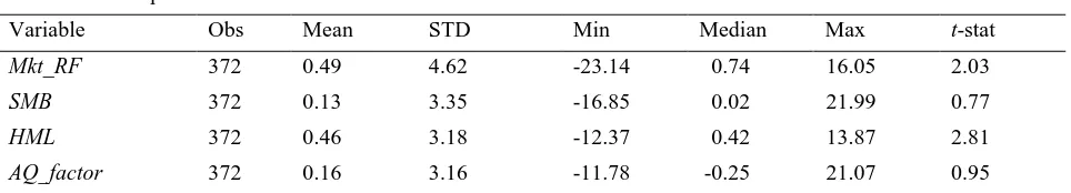
Table 1 panel A shows descriptive statistics for the AQ_factor, market risk (Mkt_RF) factor, size (SMB) factor, and book-to-market (HML) factor mimicking portfolios, the mean of each mimicking portfolio is 0.16, 0.49, 0.13 and 0.46 respectively. The mean of the each mimicking portfolio is comparable to the mean of the each mimicking portfolio in CGV which is 0.23 for AQ_factor, 0.49 for market factor, 0.13 for size factor, and 0.45 for book-to-market factor. Panel B of table 1 presents a correlation matrix. HML negatively correlates to all the other three factors. The correlations are similar to the correlations in FLOS (2005) and CGV (2008) to the four factors.
Table 1. Descriptive statistics and correlation matrix
Panel A- Descriptive statistics
Variable Obs Mean STD Min Median Max t-stat
Mkt_RF 372 0.49 4.62 -23.14 0.74 16.05 2.03
SMB 372 0.13 3.35 -16.85 0.02 21.99 0.77
HML 372 0.46 3.18 -12.37 0.42 13.87 2.81
AQ_factor 372 0.16 3.16 -11.78 -0.25 21.07 0.95
Panel B - Correlation matrix of the factors
Mkt_RF SMB HML AQ_factor
Mkt_RF 1.00 0.27 -0.46 0.35
SMB 0.27 1.00 -0.31 0.73
HML -0.46 -0.31 1.00 -0.46
AQ_factor 0.35 0.73 -0.46 1.00
4.2 Two-Stage-Cross Sectional Regressions (2SCSR)
To test whether the AQ_factor is a priced factor, we use a two-stage cross-sectional regression approach. We use a panel data model to control for cross-sectional effects in the second stage. In the second stage regressions, excess returns are regressed on risk factor betas. Our tests examine whether the AQ is a priced risk factor after controlling for the three Fama & French (1993) factors (the market risk premium (𝑅𝑚,𝑗− 𝑅𝐹,𝑗), size (SMB), and book-to-market
(HML)).
In the first stage, we estimate multivariate betas from both of a single time-series regression and rolling time-series regressions of excess returns for a firm 𝑟𝑗,𝑡− 𝑟𝐹,𝑡 on the contemporaneous returns to the Fama-French factors and
the AQ factor. The following is the first stage time-series regression:
𝑟𝑗,𝑡− 𝑟𝐹,𝑡= 𝑏𝑗,0+ 𝑏𝑗,𝑅𝑚−𝑅𝑓(𝑅𝑚,𝑗− 𝑅𝐹,𝑗) + 𝑏𝑗,𝑆𝑀𝐵𝑆𝑀𝐵𝑡+ 𝑏𝑗,𝐻𝑀𝐿𝐻𝑀𝐿𝑡 + 𝑏𝑗,𝐴𝑄𝑓𝑎𝑐𝑡𝑜𝑟𝐴𝑄𝑓𝑎𝑐𝑡𝑜𝑟𝑡 + 𝜀𝑗,𝑡 (2)
Table 2 panel A shows average coefficient estimates from the firm-specific single time-series regressions of contemporaneous excess returns on a factor returns for 21,681 time-series regressions. According to CGV (2008) and FLOS (2005), the time series regression examines the contemporaneous association between firm’s returns, adjusted for risk free rate, the AQ risk factor, and the three Fama & French (1993) factors (the market risk premium (𝑅𝑚−
𝑅𝑓), size (SMB), and book-to-market (HML)). We replicate the test and report the results in Table 2 panel A. As
Fama and French factors are 0.92, 0.54, and 0.43 similar to those reported by CGV (0.90, 0.51, and 0.36 respectively) and by FLOS (0.9, 0.64, and 0.3 respectively). In addition, the AQ_factor (0.87) is positively associated with firm-specific returns as reported in CGV (0.35) and FLOS (0.28).
Table 2 panel B presents average coefficient estimates from the firm-specific rolling time-series regressions. The coefficients (and t-stat) for the market risk factor, the size factor, book-to-market factor and AQ_factor are 0.84, 0.61, 0.49, and 0.60 which are similar to the results from single time-series regressions. Since the rolling time-series model has higher explanatory power with R2 (0.32) compared to the one in the single time-series model with R2 (0.23), we conduct our next panel regressions based on factor betas from the rolling time-series model. And also in Fama and MacBeth approach, the market betas to be used in each monthly cross-sectional regressions are usually estimated using rolling betas.
Table 2. Firm-specific, time-series regressions of contemporaneous excess returns on factor returns
Panel A- Single time-series regressions
Variable Coef t-stat Pr > |t|
Intercept -0.04 -154.21 <.0001
Mkt_RF 0.92 135.21 <.0001
SMB 0.54 42.93 <.0001
HML 0.43 35.14 <.0001
AQ_factor 0.87 51.25 <.0001
R2 0.23
N 21,681
Panel B- Rolling time-series regressions using rolling windows of 60-months returns
Coef t-stat Pr > |t|
Intercept -0.04 -16.82 <.0001
Mkt_RF 0.84 29.28 <.0001
SMB 0.61 3.42 0.0006
HML 0.49 5.38 <.0001
AQ_factor 0.60 15.71 <.0001
R2 0.32
N 2,266,388
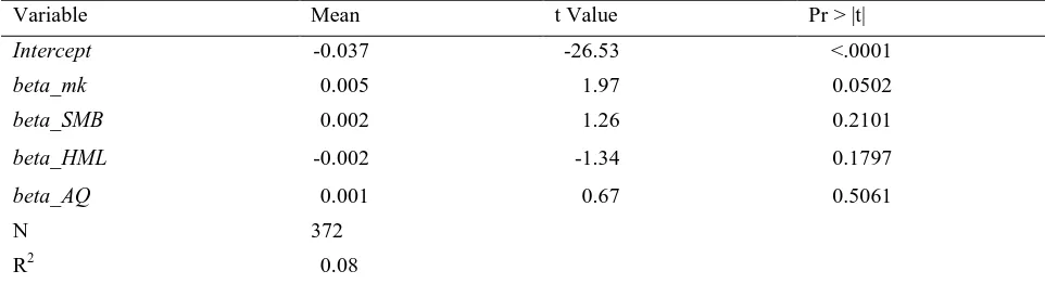
4.2.1 Averaged Cross-Section Method in the Second Stage of Fama-MacBeth Two-Stage Regressions (Replication of CGV (2008))
However, as CGV (2008) criticize, the average positive coefficient on the AQ_factor in the first pass regression does not imply that AQ is a priced risk factor. Rather, an average positive regression coefficient means that, on average, firms have a positive contemporaneous exposure to the AQ_factor mimicking portfolio on the second stage of Fama-MacBeth two-stage regressions. Following CGV, our tests examine whether AQ is a price risk factor after controlling for the three Fama & French (1993) factors (the market risk premium (𝑅𝑚− 𝑅𝑓), size (SMB), and
book-to-market (HML).
In the second stage (Eq. 3), mean excess returns are regressed on the betas of factors obtained from the first stage.
𝑟𝑗,𝑡
̅̅̅̅ − 𝑟̅̅̅̅ = 𝜆𝐹,𝑡 0+ 𝜆1𝑏𝑗,𝑅𝑚−𝑅𝑓+ 𝜆2𝑏𝑗,𝑆𝑀𝐵+ 𝜆3𝑏𝑗,𝐻𝑀𝐿+ 𝜆3𝑏𝑗,𝐴𝑄𝑓𝑎𝑐𝑡𝑜𝑟+ 𝑢𝑗 (3)
regression, the model with betas obtained from rolling time-series regressions (table 3 panel B) has higher explanatory power with R2 0.12 compared to the one in the model with betas obtained from the single time-series regressions with R2 0.08 (table 3 panel A).
Table 3. Cross-sectional regressions of excess returns on factor betas
Panel A- Betas obtained from the single time-series regressions
Variable Mean t Value Pr > |t|
Intercept -0.037 -26.53 <.0001
beta_mk 0.005 1.97 0.0502
beta_SMB 0.002 1.26 0.2101
beta_HML -0.002 -1.34 0.1797
beta_AQ 0.001 0.67 0.5061
N 372
R2 0.08
Panel B- Betas obtained from rolling time-series regressions
Variable Coef t Value Pr > |t|
Intercept -0.035 -21.95 <.0001
beta_mk 0.002 0.64 0.5224
beta_SMB 0.003 1.49 0.1373
beta_HML -0.001 -0.36 0.7220
beta_AQ 0.003 1.54 0.1237
N 313
R2 0.12
4.2.2 Panel Data Analysis in the Second Stage of Fama-MacBeth Two-Stage Regressions Controlling for the Cross-Sectional Fixed Effect
As suggested by Petersen (2009), the outcome in CGV (2008) may have been a result of using inappropriate econometric techniques. According to Wooldridge (2001), panel model is the appropriate model for the panel datasets which contain observations on multiple firms in multiple years, such as the datasets used in FLOS (2005) and CGV (2008). Following Petersen (2009), we should apply the unbalanced panel data model to our panel datasets. To calculate accurate standard error, we use the unbalanced panel data model controlling for firm-fixed effects in the second pass regression instead of estimating average cross-sectional coefficients.
We use firm-specific regressions to allow comparison with the first-stage time–series results in FLOS (2005) and CGV (2008). In the second stage (Eq.4), firm specific excess returns are regressed on the betas of factors obtained from the first stage of the rolling time-series regression and firm fixed effects (𝑐). The assumption is that C is (roughly) constant over time. Also C contains unobserved firm characteristics—such as managerial quality or structure—that can be viewed as being (rough) constant over the period (Wooldridge, 2001)
𝑟𝑗,𝑡− 𝑟𝐹,𝑡= 𝜆0+ 𝜆1𝑏𝑗,𝑅𝑚−𝑅𝑓+ 𝜆2𝑏𝑗,𝑆𝑀𝐵+ 𝜆3𝑏𝑗,𝐻𝑀𝐿+ 𝜆3𝑏𝑗,𝐴𝑄𝑓𝑎𝑐𝑡𝑜𝑟+ 𝐶𝑗+ 𝑢𝑗 (4)
Table 4. Panel regression with cross-sectional fixed effect of excess returns on factor betas
beta_mk beta_SMB beta_HML beta_AQ
Coef 0.001 0.002 0.002 0.003
t-stat 2.41 15.82 11.73 30.61
p -value 0.0158 <0.0001 <0.0001 <0.0001
Cross-sectional fixed effects: Yes
4.3 Return Decomposition Framework and Two-Stage-Cross Sectional Regressions 4.3.1 Return Decomposition Framework
Campbell (1991) decomposes the return into three components using the log-linear approximation of the dividend –price ratio derived by Campbell and Shiller (1988):
𝑟𝑡≡ 𝐸𝑡−1[𝑟𝑡] + (𝐸𝑡− 𝐸𝑡−1) ∑ 𝜌𝑖∆ 𝑑𝑡+1− (𝐸𝑡− 𝐸𝑡−1) ∑ 𝜌𝑗𝑟𝑡+𝑗 ∞
𝑗=1 ∞
𝑖=0
𝑟𝑡= 𝐸𝑡−1[𝑟𝑡] + 𝑁𝑐𝑓,𝑡− 𝑁𝑟,𝑡 (5)
Where r is the logarithm of return, 𝜌 is a linearization constant given by 1/ (1+exp (average (d-p)) and set to be 0.96 for the reminder of the study. To be consistent with CGV (2008), we use return instead. ∆𝑑 is approximately the logarithm of dividend growth. As shown in Eq.(5), the realized stock return consists of three components: the one-period expected stock return {𝐸𝑡−1[𝑟𝑡]}, the cash-flow news (𝑁𝑐𝑓,𝑡) , and the negative expected –return news
(−𝑁𝑟,𝑡).
In the spirit to Hecht & Vuolteenaho (2006), we split the Fama-MacBeth two-stage cross-sectional regression into three component regressions corresponding to the one-period expected –return, the cash-flow news, and the expected-return news. We investigate whether the AQ factor is priced in each component of excess returns.
For the traditional two-stage cross-sectional regressions, the first stage (Eq.2 aforementioned) involves a time-series regression of excess returns for a firm with a portfolio of firms (𝑟𝑡− 𝑟𝑓) on the contemporaneous returns of the Fama-French factors and the AQ factor.
In the second stage (Eq. 3 aforementioned), mean excess returns are regressed on the betas of the factors obtained from the first stage.
Using the Campbell (1991) return decomposition and following Hecht & Vuolteenaho (2006), the original second-stage regression can be decomposed into three component regressions,
𝐸𝑡−1[𝑟𝑡] = 𝜆0,𝐸𝑟+ 𝜆1,𝐸𝑟𝑏𝑗,𝑅𝑚−𝑅𝑓+ 𝜆2,𝐸𝑟𝑏𝑗,𝑆𝑀𝐵+ 𝜆3,𝐸𝑟𝑏𝑗,𝐻𝑀𝐿
+ 𝜆3,𝐸𝑟𝑏𝑗,𝐴𝑄𝑓𝑎𝑐𝑡𝑜𝑟 + 𝑢𝑗,𝐸𝑟 (6)
𝑁𝑐𝑓,𝑡= 𝜆0,𝑁𝑐𝑓+ 𝜆1,𝑁𝑐𝑓𝑏𝑗,𝑅𝑚−𝑅𝑓+ 𝜆2,𝑁𝑐𝑓𝑏𝑗,𝑆𝑀𝐵+ 𝜆3,𝑁𝑐𝑓𝑏𝑗,𝐻𝑀𝐿
+𝜆3,𝑁𝑐𝑓𝑏𝑗,𝐴𝑄𝑓𝑎𝑐𝑡𝑜𝑟+𝑢𝑗,𝑁𝑐𝑓 (7)
−𝑁𝑟,𝑡
= 𝜆0,𝑁𝑟+ 𝜆1,𝑁𝑟𝑏𝑗,𝑅𝑚−𝑅𝑓+ 𝜆2,𝑁𝑟𝑏𝑗,𝑆𝑀𝐵+ 𝜆3,𝑁𝑟𝑏𝑗,𝐻𝑀𝐿+ 𝜆3,𝑁𝑟𝑏𝑗,𝐴𝑄𝑓𝑎𝑐𝑡𝑜𝑟
+ 𝑢𝑗,𝑁𝑟 (8)
expected return is more related to macroeconomic factors. The noise component which is relatively trivial compared to the first two components and also increases information risk (Francis et al., 2005; Guay et al.,1996).
4.3.2 Estimation of One-Period Expected Returns, Cash-Flow News, and Expected-Return News
To conduct the regressions, we need to estimate the one-period expected returns, cash-flow news, and expected-return news. Campbell (1991) models the stock return as one element of a vector autoregression. Campbell (1991) begins by working with real stock returns, and then modifies the model to handle excess stock returns. In vector notation the VAR can be written as follows (Campbell, 1991; Guo, 2017):
𝑍𝑡= 𝛤𝑍𝑡−1+ 𝑢𝑡 (9)
Let Zt be a vector of state variables indicating the economy at time t. In particular, the three elements of Zt include the aggregate stock return, changes in dividends and changes in default rates. To pick off only the return series, Campbell (1991) creates a vector e1 that has a 1 as the first element and zeros elsewhere. The one-period expected return is 𝐸𝑡−1[𝑟𝑡] = 𝑒1′𝛤𝑗𝑍𝑡 . From Eq. (9) introduced by Campbell (1991), the revision in the forecast of returns
(denoted𝜂𝑟,𝑡) is equal to
𝜂r,𝑡= 𝑒1′𝜆′𝑢𝑡 (10)
Since 𝑟𝑡− 𝐸𝑡−1[𝑟𝑡] = 𝜂𝑡= 𝜂𝑑,− 𝜂r,𝑡and 𝜂𝑑,𝑡= 𝜂𝑡+ 𝜂r,𝑡, the news about cash flows can be expressed as the
residual (e.g. the unexpected return plus expected-return news):
𝜂𝑑,𝑡= (𝑒1′+ 𝑒1′𝜆)𝑢𝑡, (11)
Where 𝜆 = 𝜌𝛤(𝐼 − 𝜌𝛤)−1.
4.3.3 Empirical Results on Decomposed Returns in Two-Stage-Cross Sectional Regressions with Cross-Sectional Fixed Effects
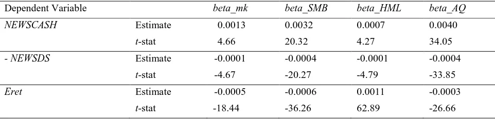
Table 5 shows the decomposition of the market returns using the panel data model controlling for the firm fixed effects. The results show that the accrual quality factor is priced in cash flow news component and offset by discount news component, but not the one-period expected return component. The coefficients (p-value) on AQ_factor related to cash flow news, discount news, and one-period expected return are equal to 0.004 (<0.0001), -0.0004 (<0.0001), and -0.0003 (<0.0001), respectively.
Table 5. Panel Regressions with cross-sectional fixed effects of decomposed excess returns on factor betas
Dependent Variable beta_mk beta_SMB beta_HML beta_AQ
NEWSCASH Estimate 0.0013 0.0032 0.0007 0.0040
t-stat 4.66 20.32 4.27 34.05
- NEWSDS Estimate -0.0001 -0.0004 -0.0001 -0.0004
t-stat -4.67 -20.27 -4.79 -33.85
Eret Estimate -0.0005 -0.0006 0.0011 -0.0003
t-stat -18.44 -36.26 62.89 -26.66
Cross-sectional fixed effects: Yes
5. Additional Tests
Following FLOS (2005), we also conduct our tests for the sample of the 7,056 firms with AQ values and return data. Table 6 presents the results for the 7,056 firms on the same tests as conducted for the 21,681 firms. One of the noticeable differences in the results for the 7,056 firms compared to the ones for the 21,681 firms is that the results for 7,056 firms regarding the estimated coefficients on beta_SMB and beta_AQ factor at the second stage of the conventional cross-sectional test are statistically significant (at 5% significance level for beta_SMB and at the 10% significance level for beta_AQ) among the estimated coefficients on the four factors. As mentioned in FLOS (2005), the results might be specific to the sample of firms which are used to calculate AQ quintile.
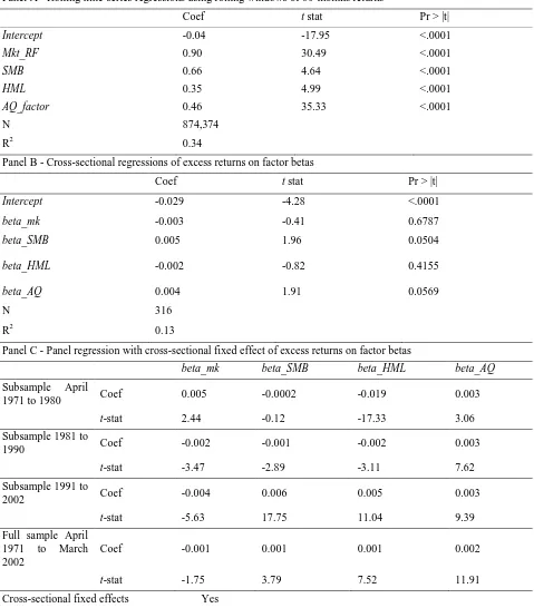
Table 6 panel A shows average coefficient estimates from the firm-specific rolling time-series regressions of contemporaneous excess returns on a factor returns for 7,056 time-series regressions. In the augmented Fama-French model with the AQ_factor, the estimated coefficients of the three Fama and French factors (the market risk premium (𝑅𝑚− 𝑅𝑓), size (SMB), and book-to-market (HML)) and AQ_factor are 0.90, 0.66, 0.35 and 0.46 similar to those reported by FLOS (0.86, 0.58, 0.32 and 0.29 respectively) for the firms with AQ value and required return data. Table 6 Panel B presents the results from conventional cross-sectional regressions of excess returns on factor betas. The estimated coefficients (p value) of the market risk beta (beta_mk), size beta (beta_SMB), book-to-market beta (beta_HML), and beta_AQ are -0.003 (0.6787), 0.005 (0.0504), -0.002 (0.4155), and 0.004 (0.0569), respectively. As noted, the estimated coefficients on beta_SMB (at 5% significance level) and beta_AQ factor (at 10% significance level) are statistically significant among the estimated coefficients on the four factors for the 7,056 firms. However, Petersen (2009) suggests that the Fama-MacBeth standard errors implemented by the firm-fixed effects perform better. To calculate accurate standard error, we implement the model with firm fixed effects to examine whether AQ_factor is priced in the excess return for the sample with AQ value. Table 6 panel C exhibits the results with the implementation of the firm- fixed effects for the full sample period from April 1971 to March 2002 as well as the three subsamples of ten years each. AQ_factor is priced in the excess return across the all sample periods: the estimated coefficients (t-stat and p value) for subsample April 1971 to 1980, 1981 to 1990, 1991 to 2002, and April 1971 to March 2002 are 0.003 (3.06 and 0.0022), 0.003 (7.62 and <0.0001), 0.003 (9.39 and<0.0001), and 0.002 (11.91 and <0.0001).
Table 6. Results for 7,056 firms with financial data and at least 18 months stock returns from April 1971 to March 2002
Panel A - Rolling time-series regressions using rolling windows of 60-months returns
Coef t stat Pr > |t|
Intercept -0.04 -17.95 <.0001
Mkt_RF 0.90 30.49 <.0001
SMB 0.66 4.64 <.0001
HML 0.35 4.99 <.0001
AQ_factor 0.46 35.33 <.0001
N 874,374
R2 0.34
Panel B - Cross-sectional regressions of excess returns on factor betas
Coef t stat Pr > |t|
Intercept -0.029 -4.28 <.0001
beta_mk -0.003 -0.41 0.6787
beta_SMB 0.005 1.96 0.0504
beta_HML -0.002 -0.82 0.4155
beta_AQ 0.004 1.91 0.0569
N 316
R2 0.13
Panel C - Panel regression with cross-sectional fixed effect of excess returns on factor betas
beta_mk beta_SMB beta_HML beta_AQ
Subsample April
1971 to 1980 Coef 0.005 -0.0002 -0.019 0.003
t-stat 2.44 -0.12 -17.33 3.06
Subsample 1981 to
1990 Coef -0.002 -0.001 -0.002 0.003
t-stat -3.47 -2.89 -3.11 7.62
Subsample 1991 to
2002 Coef -0.004 0.006 0.005 0.003
t-stat -5.63 17.75 11.04 9.39
Full sample April 1971 to March 2002
Coef -0.001 0.001 0.001 0.002
t-stat -1.75 3.79 7.52 11.91
Panel D- Cross-sectional regressions of decomposed excess returns April 1971 to March 2002
Dependent Variable
Intercept beta_mk beta_SMB beta_HML beta_AQ
NEWSCASH Coef -0.0054 0.0024 0.0039 -0.0004 0.0044
t-stat -1.93 0.6 1.73 -0.17 1.91
- NEWSDS Coef 0.0007 -0.0003 -0.0006 0.0001 -0.0005
t-stat 1.9 -0.6 -1.75 0.3 -1.6
Eret Coef -0.0003 0.0002 0.0000 0.0000 0.0001
t-stat -0.43 0.78 0.01 -0.03 1.21
Cross-sectional fixed effects No
Panel E-Panel regression with cross-sectional fixed effect of excess returns on factor betas
Dependent Variable beta_mk beta_SMB beta_HML beta_AQ
subsample April 1971 to 1980
NEWSCASH Coef 0.003 0.001 -0.019 0.003
t-stat 1.32 0.72 -15.1 3.16
- NEWSDS Coef -0.0004 -0.0001 0.003 -0.0004
t-stat -1.15 -0.54 15.28 -2.9
Eret Coef 0.002 -0.001 -0.003 -0.0001
t-stat 7.57 -5.63 -18.35 -0.32
subsample April 1981 to 1990
NEWSCASH Coef -0.002 -0.0004 -0.002 0.004
t-stat -2.3 -0.91 -3.56 9.01
- NEWSDS Coef 0.0002 0.0001 0.0003 -0.001
t-stat 2.16 0.75 3.64 -9.13
Eret Coef -0.001 -0.001 0.0002 -0.0005
t-stat -8.13 -13.53 2.58 -8.39
subsample April 1991 to 2002
NEWSCASH Coef -0.004 0.006 0.004 0.007
t-stat -5.56 10.72 9.46 17.79
- NEWSDS Coef 0.001 -0.001 -0.001 -0.001
t-stat 5.46 -10.62 -9.5 -17.71
Eret Coef -0.00004 0.00015 -0.00002 -0.00001
t-stat -0.43 2.26 -0.33 -0.22
full sample April 1971 to March 2002
NEWSCASH Coef 0.0004 0.002 0.001 0.003
t-stat 1.11 7.87 3.34 15.43
- NEWSDS Coef -0.0001 -0.0002 -0.0001 -0.0004
t-stat -1.12 -7.83 -3.49 -15.4
Eret Coef -0.0008 -0.0007 0.0008 -0.0005
t-stat -18.83 -26.41 28.06 -22.1
6. Conclusion
We find that accrual quality is a priced risk factor from the tests on the two-passing asset pricing model implemented with firm-fixed effects for the all 21,681 firms in CRSP with required return data. The rough estimations from the second stage of the conventional cross-sectional tests and the estimations from the tests implemented with firm-fixed effects for the 7,056 firms with AQ value also confirm the main findings.
More importantly, the results of the tests of the return-decomposition framework developed by Campbell & Shiller (1988a) and Campbell (1991) reveal that accrual quality is priced at a firms’ cost of capital and is priced in the cash flow news component of firms’ return. The overall results support that the firms’ information quality (proxied by the accrual quality) directly to the cost of capital through firms’ expected cash flow that does not rely on liquidity or shareholder base effects as theorized by Leuz & Verrechia (2005).
References
Aboody, D., Hughes, J., & Liu, J. (2005). Earnings quality, insider trading, and cost of capital. Journal of Accounting Research, 43, 651–673. https://doi.org/10.1111/j.1475-679X.2005.00185.x
Amihud, Y., & Mendelson, H. (1986). Asset pricing and the bid-ask spread. Journal of Financial Economics, 17, 223-249. https://doi.org/10.1016/0304-405X(86)90065-6
Armstrong, C.S., Core, J .E., Taylor , D.J., & Verrecchia, R.E. (2011). When does information asymmetry affect the cost of capital?. Journal of Accounting Research, 49, 1–40. https://doi.org/10.1111/j.1475-679X.2010.00391.x
Baltagi, B. H. (1995). Econometric Analysis of Panel Data. New York: John Wiley and Sons.
Campbell, J. Y. (1991). A Variance Decomposition for Stock Returns. Economic Journal, 101, 57–179. https://doi.org/10.2307/2233809
Campbell, J. Y., & Shiller, R. J. (1988). The Dividend-Price Ratio and Expectations of Future Dividends and Discount Factors. Review of Financial Studies, 1, 195–228. https://doi.org/10.1093/rfs/1.3.195
Core, J. E., Guay, W.R., & Verdi, R. (2008). Is accruals quality a priced risk factor? Journal of Accounting and Economics, 46, 2–22. https://doi.org/10.1016/j.jacceco.2007.08.001
Daniel, K., & Titman, S. (2006). Market Reactions to Tangible and Intangible Information. The Journal of Finance, 61, 1605–43. https://doi.org/10.1111/j.1540-6261.2006.00884.x
Dechow, P., & Dichev, I. (2002). The quality of accruals and earnings: the role of accrual Estimation errors. The Accounting Review, 77(Supplement), 35–59. https://doi.org/10.2308/accr.2002.77.s-1.35
Easley, D., & O’Hara, M. (2004). Information and the Cost of Capital. The Journal of Finance, 59, 1553-1583. https://doi.org/10.1111/j.1540-6261.2004.00672.x
Easley, D., Hvidkjaer, S., & O’Hara, M. (2010). Factoring Information into Returns. Journal of Financial and Quantitative Analysis, 45, 293–309. https://doi.org/10.1017/S0022109010000074
Fama, E., & French, K. (1993). Common risk factors in the returns on bonds and stocks. Journal of Financial Economics, 33, 3–56. https://doi.org/10.1016/0304-405X(93)90023-5
Fama, E., & MacBeth, J. (1973). Risk, return, and equilibrium: empirical tests. Journal of Political Economy, 81, 607–636. https://doi.org//10.1086/260061
Francis, J., LaFond, R., Olsson, P., & Schipper, K. (2005). The market pricing of accruals quality. Journal of accounting and economics, 39(2), 295-327. https://doi.org/10.1016/j.jacceco.2004.06.003
Guay, W. R., Kothari, S. P., & Watts, R. L. (1996). A market-based evaluation of discretionary accrual models. Journal of accounting research, 34, 83-105. https://doi.org/10.2307/2491427
Guo, Z. Y. (2017). How information is transmitted across the nations? An empirical investigation of the US and Chinese commodity markets. Global Journal of Management and Business Research, 17, 1-11.
Healy, P. (1996). Discussion of a market-based evaluation of discretionary accrual models. Journal of Accounting Research, 34, 107-115. https://doi.org/10.2307/2491428
Hecht, P., & Vuolteenaho, T. (2005). Explaining returns with cash-flow proxies. The Review of Financial Studies, 19(1), 159-194. https://doi.org/10.1093/rfs/hhj001
Kravet, T., & Shevlin, T. (2010). Accounting restatements and information risk. Review of Accounting Studies, 15(2), 264-294. https://doi.org/10.1007/s11142-009-9103-x
Leuz, C. and Verrecchia, R.E. (2005), Firms’ capital allocation choices, information quality, and the cost of capital available at: https://ssrn.com/abstract=495363
Lundblad, C. (2007). The risk return tradeoff in the long run: 1836–2003. Journal of Financial Economics, 85(1), 123-150. https://doi.org/10.1016/j.jfineco.2006.06.003
McNichols, M. F. (2002). Discussion of the quality of accruals and earnings: The role of accrual estimation errors. The accounting review, 77(s-1), 61-69. https://doi.org/10.2308/accr.2002.77.s-1.61
Ogneva, M. (2012). Accrual quality, realized returns, and expected returns: The importance of controlling for cash flow shocks. The Accounting Review, 87(4), 1415-1444. https://doi.org/10.2308/accr-10276
Petersen, M. A. (2009). Estimating standard errors in finance panel data sets: Comparing approaches. The Review of Financial Studies, 22(1), 435-480. https://doi.org/10.1093/rfs/hhn053
Wooldridge, J. (2001). Econometric Analysis of Cross Section and Panel Data. Cambridge, MA: MIT Press.
Appendix A
Definition of Key variables
Accrual quality (AQ) of a firm in the year t is calculated as the standard deviation of the firm-specific residual in Eq. (1).{ σ (𝜗𝑗,𝑡) } from year t-4 through year t (i.e. the five-year standard deviation). The higher AQ represents the
higher variation of the unexplained portion of accruals, and thus, indicates higher uncertainty in accruals, lower accounting quality, and higher information risk. Following previous research, we form an AQ factor-mimicking portfolio by taking the difference between the monthly excess returns of the top two quintiles (Q4 and Q5) and the bottom two AQ quintiles (Q1 and Q2). The AQ factor portfolio is formed monthly.
AQ_factor (AQ factor-mimicking portfolio) is measured by taking the difference between the monthly excess returns of the top two quintiles (Q4 and Q5) and the bottom two AQ quintiles (Q1 and Q2). The AQ factor portfolio is formed monthly.
Notes
Note 1. Core et al. (2008) averages cross-sectional coefficient across the sample period without considering cross-sectional fixed effect as investigated in Petersen (2009). As a result the coefficients and standard errors are biased. According to Baltagi (1995), panel data havea large number of data points, increase degrees of freedom, reduce collinearity, improve efficiency of estimates and broaden the scope of inference.
Note 2. Campbell (1991) uses this framework and a vector autoregressive (VAR) model to decompose market returns into one-period expected return (positive component), cash-flow news (positive component) and discount-rate news (negative component).