R E S E A R C H
Open Access
Black bears alter movements in response to
anthropogenic features with time of day
and season
Katherine A. Zeller
1*, David W. Wattles
2, Laura Conlee
3and Stephen DeStefano
4Abstract
Background:With the growth and expansion of human development, large mammals will increasingly encounter humans, elevating the likelihood of human-wildlife conflicts. Understanding the behavior and movement of large mammals, particularly around human development, is important for crafting effective conservation and
management plans for these species.
Methods:We used GPS collar data from American black bears (Ursus americanus) to determine how seasonal food resources and human development affected bear movement patterns and resource use across the Commonwealth of Massachusetts.
Results:We found that though bears moved more and avoided human development during crepuscular and daylight hours than at night, bears preferentially moved through human dominated areas at night. This indicates bears were mitigating the risk of human development by altering their behavior to exploit these areas when human activity is low. This behavioral shift was most prominent in the spring, when natural foods are scarce, and fall, when energetic demands are high. We also observed a high degree of inter-individual variability among our sample of bears. Bears with a higher density of houses in their home ranges (~ 75 houses/km2) displayed less avoidance of human development than more rural bears. Furthermore, bear movement models had different explanatory variables, with preference or avoidance of a variable being dependent on the individual bear. To account for this individuality in our predictive surfaces, we projected the probability of movement for each season and time of day using a spatially weighted surface centered on each bear’s home range.
Conclusions:We found that black bears in Massachusetts are operating in a landscape of fear and are altering their movement patterns to use developed areas when human activity is low. We also found seasonal and diel
differences among individual bears in resource selection during movement. Accounting for these individual, seasonal, and diel differences when assessing movement for large mammals is especially important if predictive surfaces are to be used in identifying areas for conservation and management.
Keywords:Carnivore, Conservation, Movement ecology, Human development, Multi-scale habitat selection, Massachusetts
© The Author(s). 2019Open AccessThis article is distributed under the terms of the Creative Commons Attribution 4.0 International License (http://creativecommons.org/licenses/by/4.0/), which permits unrestricted use, distribution, and reproduction in any medium, provided you give appropriate credit to the original author(s) and the source, provide a link to the Creative Commons license, and indicate if changes were made. The Creative Commons Public Domain Dedication waiver (http://creativecommons.org/publicdomain/zero/1.0/) applies to the data made available in this article, unless otherwise stated.
* Correspondence:kathyzeller@gmail.com
Background
Due to their space requirements, large mammals often exist partially or wholly outside of protected areas where they are exposed to varying levels of human presence. With the continued growth, expansion, and spatial redis-tribution of human populations, large mammals will in-creasingly encounter humans and human development [1,2]. Human development has been shown to fragment and decrease the amount of habitat [3], reduce move-ments [4], and lower rates of survival and fecundity [5] for large mammals. However, developed areas may also provide food, either in the form of non-natural foods like garbage, agricultural crops, and livestock [6], or a higher density of natural foods like forage, rodents, and deer [7]. Because large mammals, especially carnivores, living in and around developed areas have been shown to increase human-wildlife conflict [8], understanding behavior and movement of these species in areas of hu-man development is crucial for crafting effective educa-tion and management plans to reduce human-wildlife interactions.
The American black bear (Ursus americanus) is an op-portunistic omnivore that can exploit anthropogenic foods such as garbage, bird seed, fruit trees, and agricul-tural crops. In developed areas, these supplemental foods can sometimes be an additional source of nutri-tion, however, bears in these areas also have an increased likelihood of mortality from vehicle collisions and lethal removal as well as decreased survival rates for subadults and adult females [3,9–11]. A risk-reward tradeoff exists for bears living in and near human development, sug-gesting bears may be operating in a‘landscape of fear’ – a conceptual model originally developed for prey species where an individual’s perception and use of its environ-ment is the result of a cost-benefit analysis of food and risk [12–14]. Under this framework, the risk-reward tra-deoffs for black bears would not only be influenced by the built environment, but also the energetic state of an individual and the presence of conspecifics [13].
Movement patterns can express how black bears per-ceive the human environment and the risk-reward trade-off [15, 16]. Previous studies have found black bears in relatively undisturbed areas move more during diurnal and crepuscular time periods than at night [9,17], while black bears in areas of human development have been shown to shift movement activity to nocturnal periods [9,18]. Johnson et al. [19] and Baruch-Mordo et al. [20] found black bears increase use of human development and are more active at night in years when natural food is scarce. Seasonally, bears have used human develop-ment more in spring, when natural food availability is typically low [19], and in fall when bears are in a state of hyperphagia [21]. These findings suggest black bears per-ceive human areas as risky, but will utilize these areas in
times of low food availability to improve their energetic state. However, a black bear study in Pennsylvania, New Jersey, and West Virginia found no difference in re-sponse to human development between urban and rural black bears and concluded that uniform management ac-tions could be applied across the entire bear population [22].
Clearly, there are still nuances in the movement pat-terns of black bears that can shed light on their percep-tion of the risk-reward tradeoff in developed areas. The aforementioned studies have not examined movement in relation to different landscape features at different times of day, nor have they modeled movement with multi-scale models, which have been shown to be more appro-priate than single scale models for modeling movement and habitat use [23, 24]. Furthermore, these studies did not predict movement in response to human develop-ment in a spatially-explicit manner that preserves the in-dividuality of each bear and its presumed acclimation to human development [21].
Black bears have been observed to be highly individu-alistic in their response to landscape features [25]. Some of these individual responses may be the result of differ-ent genotypic or phenotypic expressions (e.g., boldness, curiosity, spatial learning) [26,27], or sex, age, or repro-ductive status [21,25, 28–30]. Other differences may be the result of acclimation to various landscape features in their home ranges [21]. Many studies account for indi-vidual variability in population-wide models by using random slopes and intercepts for individuals. Even with this approach, population models have been shown to mask individual differences, lead to weak or inconclusive responses to landscape features, and result in poor pre-dictive results [25, 31]. Furthermore, spatial predictions have been solely based on population-level models des-pite spatially inhomogeneous responses across the land-scape [32]. For example, bears in more rural areas may have a stronger negative response to roads and residen-tial areas than bears in more developed environments. Modeling bears separately and then combining individ-ual predictive surfaces into a single surface that pre-serves these spatial differences helps to avoid weak predictions and spatial biases [32].
daily movement patterns as well as daily movement pat-terns in response to environmental features across sea-sons. We assumed that preference for moving through areas of human development at times other than peak movement times was evidence of bears altering their be-havior to avoid risky situations. Second, we examined re-source selection during movement by running a multi-scale step selection function (SSF) for each individual bear for each season during the day and at night. As part of this analysis we were interested in determining if bears with more human development in their home ranges would be more acclimated to human develop-ment or instead show higher avoidance of human devel-opment. Third, we predicted the probability of bear movement across the state for each season and diel period by spatially integrating the predicted surfaces for each individual weighted by the distance from each indi-vidual’s home range. The results from our analyses can be used to better understand bear perception and use of human development, project movement into areas of
the state where bears are expanding, and provide valu-able information for bear management and mitigation of human-wildlife conflicts.
Methods Study area
The study area was in the Commonwealth of Massachu-setts, USA. Bears were collared and tracked in the cen-tral and western parts of the state (Fig. 1). To account for bears that moved beyond state borders, we buffered Massachusetts by 35 km to identify our greater study area. Spatial predictions were performed across the greater study area, but then were clipped to the state boundary.
Black bear data
Female bears were captured between 2009 and 2017 and fitted with either a Telonics Gen 3 or Gen 4 GPS collar (Any use of trade, firm, or product names is for descrip-tive purposes only and does not imply endorsement by
the U.S. Government). Most bear collars between 2012 and 2017 were programmed to acquire a fix every 15 (n= 7) or 45 (n= 69) minutes. These bears were used in the movement analyses. Bears with longer fix intervals (n= 20) were used as hold-out data to assess predictive performance of the movement models. GPS collar data for each bear (ID, fix interval, date range, etc.) are pro-vided in Additional file1: Table S1.
Bears were captured via barrel traps, free-range using dart projector, and during winter den checks. Bears were immobilized using 191 mg/ml TelazolR(Tiletamine HCl and Zolazepam HCl) at a dosage of 7 mg/kg in winter, and 229 mg/ml at a dosage of 5 mg/kg in summer, ad-ministered by a syringe on the end of a jab pole or via a tranquilizer dart. All capture, immobilization, and hand-ling procedures were performed in accordance with Uni-versity of Massachusetts, Amherst IACUC Protocols # 2011–0074, 2014–0074, and 2017–0066.
GPS fixes were examined for positional errors and the following categories of fixes were removed from the data set: (1) fixes that were unresolved, (2) fixes with a PDOP > 5 and classified as resolved QFP (uncertain) or 2D, (3) fixes with a PDOP > 20 and classified as resolved QFP (certain) or 3D. This filtering was done to minimize lo-cational error [35] and resulted in a mean loss of 3.93% (SD = 2.67%) of the data points.
Den entry and den emergence were identified by visu-ally examining the GPS points for each bear and identi-fying when movement stopped in the fall and began in the spring. Only points outside of the denning period were used in the analyses.
Environmental variables
We selected a suite of landscape variables that may affect black bear movement (Table 1). Many variables were available across the entire study area. However, some variables were mapped more accurately in Massa-chusetts by the state Bureau of Geographic Information. Since most of our GPS locations were in Massachusetts, we combined the more accurate Massachusetts layers with region-wide layers by cross-walking categories from both data sets into a single layer. All raster variables were available at a 30 m pixel resolution. Vector data were rasterized to match this resolution. Though some small land use changes have occurred between the time the GIS data were collected and when the bear GPS data were obtained, land cover types are relatively stable in bear range in Massachusetts and no sweeping changes occurred over this period [37].
Seasons
Ecologically-based seasons were identified with the clus-tering technique presented by Basille et al. [38]. This ap-proach incorporates not only movement behavior, but
also land cover attributes to account for changes in be-havior based on food availability. We identified seasons using only data from bears with a 45-min fix interval (n= 69) so that speeds and turning angles were consist-ent. Data cleaning and missed GPS collar fixes resulted in the time between some locations being longer than the original collar schedule, therefore, we further subset the data so that only consecutive fixes were used. We then calculated movement speed and turning angle among consecutive points for each bear and assessed whether each point was located in coniferous forest, de-ciduous forest, forested wetland, or agricultural areas. We also determined the value of percent impervious surface at each point. At the recommendation of Basille et al. [38], we then smoothed the movement and habitat variables for each bear-year with a 5-day moving window and range standardized the data. We used k-means clus-tering and selected the number of clusters with the gap statistic [38]. This approach resulted in three seasons: spring (den emergence to June 14th), summer (June 15th to August 9th), and fall (August 10th to den entry). For the seasonal analyses presented below, only bears that had a full season’s worth of data were used.
Movement steps
Because our interest was in longer movements across the landscape, as opposed to short distance or foraging movements, we identified movement behavior from the step length and turning angle distributions of each bear by using hidden Markov models with the R package [39]
moveHMM [40]. We ran a three-state hidden Markov model which characterized behavior as (1) an encamped state with short steps and wider turning angles, (2) a for-aging state with slightly longer steps and smaller turning angles, and (3) a movement state with long step lengths and directed movement (more details and an example are provided in Additional file 2: Figure S2). We used only movement steps for all subsequent analyses.
Statistical analyses
Daily movement and habitat selection
in an individual’s seasonal home range. The boot-strapped mean and confidence intervals for each 45-min time period were calculated across bears.
Multi-scale step selection functions (SSF)
Due to differences observed in bear temporal movement and habitat selection, we ran two SSFs for each season, one with daytime points and one with nighttime points. Day/night periods for each bear were identified using daily sunrise/sunset times for Amherst, Massachusetts from the Astronomical Applications Department of the
U.S. Navy Observatory. We also ran a single SSF with all the bear data across seasons and diel periods. Bears with the 15-min or 45-min fix interval were used for this analysis.
Following Zeller et al. [23], the mean value (for con-tinuous variables) or proportion of the area (for categor-ical variables) was extracted within a 30 m uniform buffer around each step. This was the‘used’data for the SSFs. We examined multiple scales for representing the
‘available’data. Scales were determined by estimating the mean distance moved over the following time periods:
Table 1Environmental variables used in the black bear movement analyses
Variable Massachusetts source Buffer area source (if different from
Massachusetts source)
Topographic
Ruggedness derived from National Elevation Dataset
Slope derived from National Elevation Dataset
Development
All Roads Designing Sustainable Landscapes
Primary Roads Designing Sustainable Landscapes
Secondary & Tertiary Roads Designing Sustainable Landscapes
Primary, Secondary, & Tertiary Roads
Designing Sustainable Landscapes
Open space Massachusetts GIS Land Use 2005 layer (cemetery, golf course, recreation areas)
Designing Sustainable Landscapes (developed open space)
Commercial / Industrial
Massachusetts GIS Land Use 2005 layer (Commercial / Industrial / Junkyard / Urban Public, Institutional / waste disposal)
Designing Sustainable Landscapes (developed high intensity)
High density residential
Massachusetts GIS Land Use 2005 layer (Housing on < 1/4 acre lots) Designing Sustainable Landscapes (developed high intensity)
Medium density residential
Massachusetts GIS Land Use 2005 layer (Housing on 1/4–1/2 acre lots) Designing Sustainable Landscapes (developed medium intensity)
Low density residential Massachusetts GIS Land Use 2005 layer (Housing on 1/2–1 acre lots) Designing Sustainable Landscapes (developed low intensity)
Very low density residential
Massachusetts GIS Land Use 2005 layer (Housing on > 1 acre lots) Designing Sustainable Landscapes (developed low intensity)
Percent impervious surface
Designing Sustainable Landscapes
Agriculture Massachusetts GIS Land Use 2005 layer (pasture, cropland, orchard, open land)
Designing Sustainable Landscapes (pasture)
Powerline corridors Massachusetts GIS Land Use 2005 layer Designing Sustainable Landscapes (developed open space)
Water and wetlands
Open water Massachusetts GIS Land Use 2005 layer Designing Sustainable Landscapes
Emergent wetland USGS National Wetlands Inventory
Forested wetland USGS National Wetlands Inventory
Vegetation
Coniferous forest Pasquarella et al. [36]; Pasquarella et al. (in prep)
Deciduous forest Pasquarella et al. [36]; Pasquarella et al. (in prep)
Mixed forest Pasquarella et al. [36]; Pasquarella et al. (in prep)
Landscape Configuration Metrics
45 min, 1.5 h, 2.25 h, 3 h, 4.5 h, and 6 h. The mean move-ment distances were 360 m, 650 m, 837 m, 1007 m, 1288 m, and 1523 m respectively. The scales were used as the standard deviation for a Gaussian kernel placed over each step. The mean value or proportion of each variable was calculated within the Gaussian weighted kernel around each step at each scale and were used as the
‘available’ data. Used and available data were z-score standardized prior to modeling.
We modeled each bear independently to preserve indi-vidual differences and predict the relative probability of movement in a spatially unbiased manner (see Predictive Surfaces below) [32]. We paired each used step with its corresponding available step at a scale and ran paired lo-gistic regressions with the clogit function from the R package coxme [43]. For each bear, we used a two-step approach to generate the SSF [24]. We first ran univari-ate models for each variable at each scale. We identified the scale with the lowest AICc value as the characteristic scale of selection for that variable. We then assessed pairwise correlations between the variables at their char-acteristic scales. If pairwise correlations were | > 0.7|, we selected the variable from each pair with the lower AICc value for inclusion in the multiple regression models. We ran a forward and backward stepwise model selec-tion and identified the final model for each bear as the model with the lowest AICc value.
Home range housing density effects on selection
To determine if bears living in more developed areas were more acclimated to human development, we mod-eled the standardized regression coefficient for percent impervious surface as a function of home range housing density (HRHD) [21]. We calculated HRHD for each bear’s annual home range as well as each bear’s seasonal home range. For each season, we explored a linear rela-tionship and a logistic relarela-tionship. We also ran an inter-cept only model. Competing models were ranked with AICc values. We assumed that if the highest ranked model included HRHD as a variable and that if the slope of this model was positive, then bears were acclimating to residential areas within their home ranges.
Predictive surfaces
Because we observed significant results from our HRHD analysis, we concluded that bears in more developed areas were responding to landscape features differently than bears in undeveloped areas. To maintain this indi-vidual variability in our predictive surfaces we did not average the model coefficients across bears (which does not maintain individual variability in the predictive sur-face), but instead used the approach presented in Osi-pova et al. [32], which spatially weights predictions for each individual based on their home range centroid. By
projecting each bear model separately across the study area, but combining them through a spatial weighting by distance from home range centroid, a single surface is obtained. To generate this predictive surface, we used the following procedure. For each bear year, we pre-dicted the relative probability of movement across Mas-sachusetts using the exponentiated form of the relative predicted resource selection probabilities as recom-mended by Johnson et al. [44]:w^ ðxÞ ¼ expðβ1x1þβ2x2
þβ3x3þ … +βpxp). Before combining bear years into a
single surface, we weighted each bear’s surface so that areas close to each bear’s home range had a higher weight than areas further away. We implemented this by (1) estimating a kernel density home range for each bear for each season (Additional file 3), (2) identifying the home range centroid, (3) generating a distance from home range centroid surface, and (4) taking the inverse of the distance surface so that higher values were closer to the home range centroid [32]. This was our weighted surface. Each pixel on the landscape was normalized so that all the home range weighted surfaces summed to one. We then multiplied each relative predictive surface for each bear by the home range weighted surface and summed them to obtain a final predicted probability sur-face across the state for all seasons and for each season/ diel period.
We evaluated the performance of the predictive surfaces using the hold-out data set of 20 bears and calculating the Boyce Index [45,46], which compares the predicted values at the hold-out points with the expected values across the study area. The Boyce Index has values ranging from 0 to 1 with values closer to 1 indicating better predictive abil-ity. We compared the predictive surfaces with each other by calculating the Pearson’s correlation coefficient and by the pixel by pixel differences between the surfaces.
Results
Daily movement and habitat selection
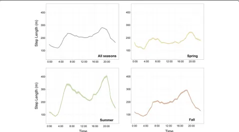
Across seasons, bears moved an average of 200 m every 45-min during daylight hours (Fig. 2). Movement steps were longer during crepuscular periods with the longest steps observed during the evening hours from approxi-mately 16:00–21:00 h. The minimum movement lengths occurred from approximately 02:00–03:00 h and remained low during most nighttime hours. Seasonally, movement activity maintained the same general patterns, but bear steps were shorter during the spring than during other times of year and were longer during summer than during other times of year (Fig.2).
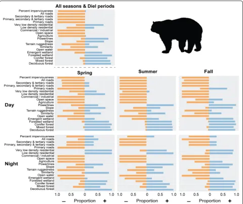
spring and summer, but bears selected for agriculture in the fall during the nighttime hours and showed variable selection in the fall during the daytime. Agriculture in our study area includes crops like corn, berries, apples, and a wide variety of vegetables bears may be utilizing. Bears had similar responses to roads and human devel-opment; bears selected for roads and residential areas at night during spring and fall, but strongly avoided these areas during the day. Bears mostly selected against roads and residential areas in the summer at all times of day with the exception of showing a slight tolerance for resi-dential areas at night.
Multi-scale step selection functions
The multi-scale SSF models for individual bears often contained different variables and different numbers of variables. The all-seasons model for each bear included 3 to 11 landscape variables with an average of 7.68 ± 1.84 variables per model. For the natural cover types, forested wetland was present in 80% of the models, and mixed and deciduous forest were both present in 73% of the models (Table2). For the developed cover types, per-cent impervious surface was present in 61% of the models, agriculture was present in 55% of the models, and the other variables were included in the bear models less often. High and medium density residential variables were not selected for any final bear model, though low and very low density residential variables were present in some of the models. Similar results were observed for
each season/diel period with forested wetland, mixed and deciduous forest, impervious surface, and agricul-ture being present in a high number of models (Table2). Bears also responded to different landscape variable scales (Additional file 4: Figure S4). Across seasons and times of day, bears typically selected for finer scales of forested wetland, conifer forest, primary roads, and com-mercial/industrial lands and selected for coarser scales of emergent wetland, agriculture, low and very low dens-ity residential areas, imperviousness, secondary and ter-tiary roads, deciduous and mixed forest, slope, and ruggedness. However, the scale of selection was not con-sistent across bears and individual bears selected varying scales for all landscape variables (Additional file 4: Fig-ure S4).
development. For spring and summer during both day and night, bear models all showed an avoidance of agri-culture, but for fall day, about 25% of models showed a preference for agriculture and for fall night, almost 50% of bear models showed a preference for agriculture.
Home range housing density analysis
Bears with a higher HRHD showed weaker avoidance of human development compared with more rural bears (Fig. 5). The logistic model was the best fitting model and was significant. AICc values of the logistic model, the linear model and the intercept only model were− 10.5, −3.8, and 5.3 respectively. The threshold of this
curve was observed around a housing density of 75–100 houses/km2. Because the percent impervious surface variable was not included in all the bear models, when we parsed the data into seasons, we did not have enough data to fit the HRHD models to each season.
Probability of movement surfaces
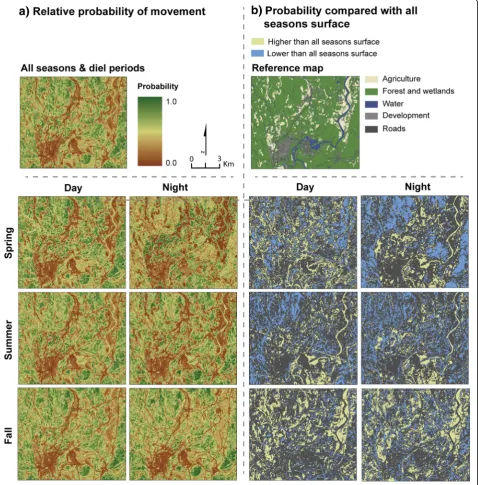
night = 0.62, summer day = 0.98, summer night = 0.86, fall day = 0.98, fall night = 0.94). However, differences be-tween the surfaces on a pixel by pixel basis could be quite pronounced. Figure 6b shows the top 20th quan-tiles of positive and negative differences between the all seasons/diel periods surface and the other surfaces. Posi-tive differences indicate that a higher probability of se-lection was observed for the pixels in that season/diel period than in the all seasons model. Negative differ-ences indicate that a lower probability of selection was observed for that season/diel period. Positive differences in relative probability values ranged from 0.05 to 0.47 for daytime surfaces and 0.09 to 0.54 for nighttime sur-faces. Negative differences in relative probability values ranged from−0.05 to−0.45 for daytime surfaces and− 0.12 to−0.92 for nighttime surfaces.
All the predictive surfaces had relatively high predict-ive performance. The Boyce Index Spearman rank cor-relation coefficient values were 0.98, 0.95, 0.72, 0.98, 0.83, 0.98, and 0.93 for the all seasons, spring day, spring night, summer day, summer night, fall day, and fall night surfaces respectively.
Discussion
In keeping with the ‘landscape of fear’ model [12, 14], our study on bear movement patterns indicates that
black bears in Massachusetts mitigate the risk of being in areas of human development by altering their behav-ior to exploit these areas when human activity is low. Nocturnal utilization of developed areas was strongest in the spring, when natural foods are more limited, and in the fall, when bears are in a state of hyperphagia. Our study also found that bears with higher amounts of hu-man development in their home ranges did not avoid human areas as strongly as more rural bears, indicating bears are acclimating to living in developed areas. Given the differences among bears living in rural and more de-veloped areas, our spatial predictions of black bear movement preserved the individual nature of bears ex-posed to different landscape features.
Black bear movement patterns were typical of black bears in wildland areas with most movement occurring during the day, with peaks during morning and evening hours [9,17]. However, examining daily selection for dif-ferent landscape features showed that when bears did move at night, they displayed a preference for roads and residential areas, especially in the spring and fall. This is a shift from normal activity patterns and suggests behav-ioral plasticity in response to human development. Simi-lar nocturnal shifts have been observed in other black bear studies in developed areas [9, 18–20]. Black bears may be shifting their use of developed areas to times
Table 2Proportion of bear models containing each environmental variable. Because the step selection functions were optimized for each individual bear, not all bears had the same explanatory variables in their final models
All seasons/diel periods Spring day Spring night Summer day Summer night Fall day Fall night
Percent impervious surface 0.61 0.29 0.14 0.55 0.33 0.35 0.30
All Roads 0.17 0.34 0.19 0.13 0.19 0.28 0.30
Secondary & Tertiary Roads 0.10 0.15 0.14 0.17 0.13 0.15 0.11
Primary, Secondary, & Tertiary Roads 0.11 0.16 0.14 0.13 0.19 0.21 0.15
Primary Roads 0.06 0.05 0.05 0.02 0 0.07 0
Very low density residential 0.14 0.24 0.38 0.21 0.19 0.12 0.26
Low density residential 0.18 0.11 0.43 0.19 0.14 0.12 0.22
Commercial / Industrial 0.23 0.21 0.29 0.17 0.10 0.09 0.07
Open space 0.14 0.05 0.24 0.06 0.05 0.05 0.11
Agriculture 0.55 0.47 0.48 0.43 0.43 0.40 0.48
Powerline corridors 0.30 0.05 0.14 0.32 0.14 0.19 0.22
Slope 0.48 0.34 0.29 0.30 0.24 0.37 0.26
Ruggedness 0.52 0.26 0.24 0.49 0.33 0.47 0.33
Similarity 0.48 0.53 0.43 0.34 0.38 0.56 0.48
Open water 0.26 0.21 0.48 0.15 0.14 0.14 0.19
Emergent wetland 0.44 0.50 0.48 0.43 0.24 0.23 0.30
Forested wetland 0.80 0.53 0.29 0.64 0.24 0.81 0.52
Coniferous forest 0.55 0.39 0.43 0.34 0.33 0.35 0.33
Mixed forest 0.66 0.47 0.38 0.44 0.57 0.53 0.44
when human activity is low, indicating black bears per-ceive human activity and associated noise and traffic as risky and may be responding to these environmental cues more than human infrastructure on the landscape [21, 47]. These shifts are not only occurring in black bears, but have also been documented in other species. In a meta-analysis on 62 species, Gaynor et al. [48] found that large mammals significantly increased noc-turnal activity in response to all types of human presence.
Limitations of natural food sources as well as the ener-getic state of individual bears may drive when bears are willing to utilize riskier human dominated areas. We found black bear use of developed areas at night was strongest in the spring and fall, indicating these behav-ioral shifts can be dynamic throughout the year and may
[19] found use of human development was also dependent on sex and age, and Evans et al. [21] found use of development was a function of reproductive sta-tus, lending further evidence that use of human develop-ment is temporally dynamic. Expanding this research to include male bears as well as bears in different age clas-ses and reproductive states would allow for a more nuanced picture of black bear response to human devel-opment in Massachusetts. Additionally, this research could be enhanced by using time of day as a continuous variable in the SSF models instead of using a binary clas-sification of day and night.
The unit of inference for our SSF analysis was the step between consecutive GPS collar fixes. Previous studies have found that as the time between fixes increases, the paths of individuals become less tortuous and shorter in length [49], and biases may be introduced into SSFs at fix rates of one hour or more [23]. Our steps were at 15 and 45-min intervals and though this period may not be short enough to completely capture the more tortuous bear movements, we are confident in our inferences. The results are biologically meaningful and echo previ-ous research on bear habitat use and movement.
Bears with a higher housing density in their home ranges had a significantly weaker avoidance of impervi-ous surfaces, indicating bears were acclimating to human development. This relationship was best expressed as a threshold, where weaker avoidance was observed at home range housing densities above approximately 75 houses/km2
. Evans et al. [21] also found a significant re-lationship between home range housing density and de-velopment and that bears showed a preference for development when their home range housing density was over 66 houses/km2. In our study, bears did not show preference, but instead, weaker avoidance with
home range housing density. Differences among these studies are likely due to the use of different measures of development. Evans et al. [21] used housing density whereas we used percent impervious surface, which is not restricted to buildings, but includes roads and other surfaces associated with development. Furthermore, our sample of bears included bears in areas that were more highly developed than those in the Evans et al. [21] study.
Bears in Massachusetts showed a high degree of inter-individual variability. Not only were bears in human dominated areas more acclimated to development than other bears, but also movement of individual bears was driven by different landscape features. Bear movement models had different numbers and types of variables and preference or avoidance of a variable was dependent on the individual bear. In general, bear movement was facil-itated by forest and forested wetland and impeded by roads and developed areas, but this was not entirely con-sistent across the population especially when seasonality and time of day was considered. Lesmerises and St-Laurent [25] observed individuality in black bears and found opposite selection coefficients that were linked to individual characteristics. They also found that when all bears were included in a population-level model, these opposite responses cancelled each other out and resulted in weak selection responses. For an omnivorous, gener-alist species such as the black bear, that is capable of be-havioral plasticity depending on its environment, ignoring individual variability can result in inconclusive or misleading results [25].
Accounting for individual variability by modeling each individual separately provides important insights for un-derstanding wildlife habitat use and movement. How-ever, applying individual models in a spatially explicit manner to project habitat use or movement across a study area is impractical due to the sheer number of in-dividual surfaces this would produce. This has prevented the use of individual models in spatially projecting re-source use and movement. Osipova et al. [32] provides a nice solution to this problem with an approach that maintains the individuality of each bear relative to its lo-cation in a study area. By projecting each bear model separately across the study area, but combining them through a spatial weighting by distance from home range centroid, a single surface is obtained. Osipova et al. [32] demonstrated that this spatial weighting ap-proach outperformed the surface derived from a popula-tion level model where the regression coefficients were averaged. We implemented the Osipova et al. [32] ap-proach and produced predictive movement surfaces spatially weighted by each individual bear. The high Boyce Index values indicate high predictive performance of these models. Because the individual-based spatially Fig. 5Logistic relationship between the home range housing
weighted approach is still a relatively new method, more research is needed to determine how many individuals and over what spatial configuration is‘enough’ to result in meaningful predictions. Additionally, Signer et al. [50], recommended a simulation-based approach for generating the predictive surfaces from SSF models as
generated from SSFs, however more research on this topic is needed.
Accounting for time of day and season was also im-portant in our predictive surfaces. Bear movement may be interpreted differently depending on the time of day and season and it is important to account for these dif-ferences when assessing movement across the landscape, especially if predictive surfaces are to be used in identify-ing areas of connectivity, conservation corridors, and road crossing locations.
Conclusions
Understanding the movement of large mammals in and around areas of human development is crucial for devel-oping successful management plans and mitigation ap-proaches for reducing human wildlife conflict. We analyzed black bear movement in the third most densely populated state in the U.S. and observed behavioral plas-ticity and acclimation to human development. We also observed inter-individual differences and suggest main-taining these inter-individual differences when spatially predicting movement across a landscape. We were un-able to assess whether use of developed areas conferred positive or negative fitness benefits, but this is a question for future research. Our results offer insights into the landscape of fear for black bears and what drives their spatial and temporal use of human dominated areas and may be used by managers across highly developed land-scapes, such as the state of Massachusetts. Our predict-ive surfaces will also help identify how and where bears are expanding as they move closer to the Boston metro-politan area.
Additional files
Additional file 1:Table S1.Bear-specific GPS collar data. (DOCX 24 kb)
Additional file 2:Figure S2.Example results from a three-state hidden Markov model for a single bear. (DOCX 441 kb)
Additional file 3:Kernel Density Home Range Estimation (DOCX 14 kb)
Additional file 4:Figure S4: Spatial scales of selection for black bear step selection functions. (DOCX 655 kb)
Additional file 5:Figure S5:Relative probability of black bear movement across the state of Massachusetts (DOCX 1689 kb)
Abbreviations
HRHD:Home range housing density; SSF: Step selection function
Acknowledgements
We wish to thank E. Van Cleave for insightful discussions on analyses and V. Pasquarella for remotely sensed forest data. We are grateful to D. Fuller, M. Morelly, N. Buckhout, and other Massachusetts Division of Fisheries & Wildlife biologists, field technicians, and managers for assistance with field work as well as Massachusetts Cooperative Fish and Wildlife Research Unit technicians J. Bonafini and H. Moylan. We would also like to thank C. Sun and the three anonymous reviewers for providing helpful and constructive feedback on this manuscript. Any use of trade, firm, or product names is for descriptive purposes only and does not imply endorsement by the U.S. Government.
Authors’contributions
DW, LC, and SD initiated and conducted the field work and DW and LC collected the telemetry data. KZ and DW conceived the manuscript idea and KZ processed the data and performed all the data analyses. KZ wrote the manuscript with contributions and input from DW and SD. All authors approved of the final manuscript submission.
Funding
This work was supported by the Massachusetts State Wildlife Grants program (W-35-R) in cooperation with the United States Fish and Wildlife Service, Wildlife, and Sport Fish Restoration Program; the Massachusetts Division of Fisheries and Wildlife; the Massachusetts Division of Conservation and Recreation; and the Massachusetts Department of Transportation.
Availability of data and materials
The data are available upon request from the authors.
Ethics approval and consent to participate
Bear capture and handling was approved by the University of Massachusetts, Amherst Institutional Animal Care and Use Committee Protocol # 2011–0074, 2014–0074, and 2017–0066.
Consent for publication
Not applicable.
Competing interests
The authors declare that they have no competing interests.
Author details
1Massachusetts Cooperative Fish and Wildlife Research Unit, University of Massachusetts, 160 Holdsworth Way, Amherst, MA 01003, USA. 2Massachusetts Division of Fisheries and Wildlife, Westborough, MA, USA. 3
Missouri Department of Conservation, Columbia, MO, USA.4U.S. Geological Survey, Massachusetts Cooperative Fish and Wildlife Research Unit, University of Massachusetts, Amherst, MA, USA.
Received: 7 March 2019 Accepted: 28 May 2019
References
1. Barnosky AD, Hadly EA, Bascompte J, Berlow EL, Brown JH, Mikael F, Getz WM, Harte J, Hastings A, Marquet PA, Martinez ND, Mooers A, Roopnarine P, Vermeij G, Williams JW, Gillespie R, Kitzes J, Marshall C, Matzke N, Mindell DP, Revilla E, Smith AB. Approaching a state shift in Earth’s biosphere. Nature. 2012;486:52–8.
2. Ripple WJ, Estes JA, Beschta RL, Wilmers CC, Ritchie EG, Hebblewhite M, Berger J, Elmhagen B, Letnic M, Nelson MP, Schmitz OJ, Smith DW, Wallach AD, Wirsing AJ. Status and ecological effects of the world’s largest carnivores. Science. 2014;343:1241484.
3. Crooks KR, Burdett CL, Theobald DM, King SRB, Marco MD, Rondinini C, Boitani L. Quantification of habitat fragmentation reveals extinction risk in terrestrial mammals. PNAS. 2017;114:7635–40.
Wittemyer G, Zięba F, Zwijacz-Kozica T, Mueller T. Moving in the Anthropocene: Global reductions in terrestrial mammalian movements. Science. 2018;359:466–9.
5. Hansen AJ, Knight RL, Marzluff JM, Powell S, Brown K, Gude PH, Jones K. Effects of exurban development on biodiversity: patterns, mechanisms, and research needs. Ecol Appl. 2005;15:1893–905.
6. Oro D, Genovart M, Tavecchia G, Fowler MS, Martinez-Abrain A. Ecological and evolutionary implications of food subsidies from humans. Ecol Lett. 2013;16:1501–14.
7. Gaughan CR, DeStefano S. Movement patterns of rural and suburban white-tailed deer in Massachusetts. Urban Ecosystems. 2005;8:191–202.
8. Treves A, Karanth KU. Human-carnivore conflict and perspectives on carnivore management worldwide. Conserv Biol. 2003;17:1491–9. 9. Beckmann JP, Berger J. Rapid ecological and behavioural changes in
carnivores: the responses of black bears (Ursus americanus) to altered food. J Zool. 2003;261:207–12.
10. Hostetler JA, McCown JW, Garrison EP, Neils AM, Barrett MA, Sunquist ME, Simek SL, Oli MK. Demographic consequences of anthropogenic influences: Florida black bears in north-Central Florida. Biol Conserv. 2009;142:2456–63.
11. Beckmann JP, Lackey CW. Carnivores, urban landscapes, and longitudinal studies: a case history of black bears. Hum-Wildl Conflicts. 2008;2:168–74. 12. Laundre JW, Hernandez L, Ripple WJ. The landscape of fear: ecological
implications of being afraid. Open Ecol J. 2010;3:1–7.
13. Bleicher SS. The landscape of fear conceptual framework: definition and review of current applications and misuses. PeerJ. 2017;5.
14. Gaynor K, Brown JS, Middleton AD, Power ME, Brashares J. Landscapes of fear: Spatial patterns of risk perception and response. Trends Ecol Evol. 2019. https://doi.org/10.1016/j.tree.2019.01.004.
15. Frid A, Dill LM. Human-caused disturbance stimuli as a form of predation risk. Conserv Ecol. 2002;6:11.
16. Fortin D, Beyer HL, Boyce MS, Smith DW, Duchesne T, Mao JS. Wolves influence elk movements: behavior shapes a rrophic cascade in Yellowstone National Park. Ecology. 2005;86:1320–30.
17. Lewis JS, Rachlow JL. Activity patterns of black bears in relation to sex, season, and daily movement rates. West N Am Nat. 2011;71:388–95. 18. Matthews SM, Beecham JJ, Quigley H, Greenleaf SS, Leithead HM. Activity
patterns of American black bears in Yosemite National Park. Ursus. 2006;17:30–40. 19. Johnson HE, Breck SW, Baruch-Mordo S, Lewis DL, Lackey CW, Wilson KR,
Broderick J, Mao JS, Beckmann JP. Shifting perceptions of risk and reward: dynamic selection for human development by black bears in the western United States. Biol Conserv. 2015;187:164–72.
20. Baruch-Mordo S, Wilson KR, Lewis DL, Broderick J, Mao JS, Breck SW. Stochasticity in natural rorage production affects use of urban areas by black bears: implications to management of human-bear conflicts. PLoS One. 2012;9:e85122.https://doi.org/10.1371/journal.pone.0085122. 21. Evans MJ, Hawley JE, Rego PW, Rittenhouse TAG. Hourly movement
decisions indicate how a large carnivore inhabits developed landscapes. Oecologia. 2018.https://doi.org/10.1007/s00442-018-4307-z.
22. Tri AN, Edwards JW, Strager MP, Petty JT, Ryan CW, Carpenter CP, Ternent MA, Carr PC. Habitat use by American black bears in the urban–wildland interface of the mid-Atlantic, USA. Ursus. 2016;27:45–56. 23. Zeller KA, McGarigal K, Cushman SA, Beier P, Vickers TW, Boyce WM. Using
step and path selection functions for estimating resistance to movement: pumas as a case study. Landsc Ecol. 2015;31:1319–35.
24. McGarigal K, Zeller KA, Cushman SA. Multi-scale habitat selection modeling: introduction to the special issue. Landsc Ecol. 2016;31:1157–60.
25. Lesmerises R, St-Laurent M-H. Not accounting for interindividual variability can mask habitat selection patterns: a case study on black bears. Oecologia. 2017;185:415–25. 26. Ioannou CC, Payne M, Krause J. Ecological consequences of the bold–shy
continuum: the effect of predator boldness on prey risk. Oecologia. 2008;157:177. 27. Heppenheimer E, Brzeski KE, Hinton JW, Patterson BR, Rutledge LY,
DeCandia AL, Wheeldon T, Fain SR, Hohenlohe PA, Kays R, White BN, Chamberlain MJ, vonHoldt BM. High genomic diversity and candidate genes under selection associated with range expansion in eastern coyote (Canis latrans ) populations. Ecol Evol. 2018;8:12641–55.
28. Lyons AJ. Activity patterns of urban American black bears in the San Gabriel Mountains of Southern California. Ursus. 2005;16:255–62.
29. Ditmer MA, Garshelis DL, Noyce KV, Laske TG, Iaizzo PA, Burk TE, Forester JD, Fieberg JR. Behavioral and physiological responses of American black bears to landscape features within an agricultural region. Ecosphere. 2015;6:28.
30. Karelus DL, McCown JW, Scheick BK, van de Kerk M, Bolker BM, Oli MK. Effects of environmental factors and landscape features on movement patterns of Florida black bears. J Mammal. 2017;98:1463–78.
31. Gillies CS, Hebblewhite M, Nielsen SE, Krawchuk MA, Aldridge CL, Frair JL, Saher DJ, Stevens CE, Jerde CL. Application of random effects to the study of resource selection by animals. J Anim Ecol. 2006;75:887–98.
32. Osipova L, Okello MM, Njumbi SJ, Ngene S, Western D, Hayward MW, Balkenhol N. Using step-selection functions to model landscape connectivity for African elephants: accounting for variability across individuals and seasons. Anim Conserv. 2019;22:35–48.
33. U. S. Census Bureau. Census 2010. Resident Population Data: Population Density. 2010. https://www.census.gov/data/tables/2010/dec/density-data-text.html
34. Massachusetts division of fisheries and wildlife. Black bears in Massachusetts. Commonwealth of Massachusetts. 2018. https://www.mass.gov/black-bears-in-massachusetts. Accessed 4 Jan 2019.
35. Lewis JS, Rachlow JL, Garton EO, Vierling LA. Effects of habitat on GPS collar performance: using data screening to reduce location error. J Appl Ecol. 2007;44:663–71.
36. Pasquarella VJ, Holden CE, Woodcock CE. Improved mapping of forest type using spectral-temporal Landsat features. Remote Sens Environ. 2018;210: 193–207.
37. Lautzenheiser T, Collins J, Ricci EH, Clarke J. Losing ground: planning for resilience. Massachusetts Audubon 2014.https://www.massaudubon.org/ content/download/12560/197561/file/MassAudubon_LosingGround5_ FINAL_medres.pdf. Accessed 5/1/2019.
38. Basille M, Fortin D, Dussault C, Ouellet J-P, Courtois R. Ecologically based definition of seasons clarifies predator-prey interactions. Ecography. 2013;36: 220–9.
39. R Core Team. R: a language and environment for statistical computing. Vienna, Austria: R Foundation for Statistical Computing; 2017.https://www. R-project.org
40. Michelot T, Langrock R, Patterson TA. moveHMM: an R package for the statistical modelling of animal movement data using hidden Markov models. Methods Ecol Evol. 2016;7:1308–15.
41. Van Cleave EK, Bidner LR, Ford AT, Caillaud D, Wilmers CC, Isbell LA. Diel patterns of movement activity and habitat use by leopards (Panthera pardus pardus) living in a human-dominated landscape in Central Kenya. Biol Conserv. 2018;226:224–37.
42. Johnson DH. The comparison of usage and availability measurements for evaluating resource preference. Ecology. 1980;61:65–71.
43. Therneau TM. coxme: Mixed effects cox models. R package version 2.2–10. 2018.https://CRAN.R-project.org/package=coxme
44. Johnson CJ, Nielsen SE, Merrill EH, McDonald TL, Boyce MS. Resource selection functions based on use-availability data: theoretical motivation and evaluation methods. J Wildl Manag. 2006;70:347–57.
45. Boyce MS, Vernier PR, Nielsen SE, Schmiegelow FKA. Evaluating resource selection functions. Ecol Model. 2002;157:281–300.
46. Hirzel AH, Le Lay G, Helfer V, Randin C, Guisan A. Evaluating the ability of habitat suitability models to predict species presences. Ecol Model. 2006; 199:142–52.
47. Ditmer MA, Rettler SJ, Fieberg JR, Iaizzo PA, Laske TG, Noyce KV, Garshelis DL. American black bears perceive the risks of crossing roads. Behav Ecol. 2018;29:667–75.
48. Gaynor KM, Hojnowski CE, Carter NH. The influence of human disturbance on wildlife nocturnality. Science. 2018;360:1232–5.
49. Mills KJ, Patterson BR, Murray DL. Effects of variable sampling frequencies on GPS transmitter efficiency and estimated wolf home range size and movement distance. Wildl Soc Bull. 2016;34:1463–9.
50. Signer J, Fieberg J, Avgar T. Estimating utilization distributions from fitted step selection functions. Ecosphere. 2017;8:e01771.
Publisher’s Note