Page 1 of 11
Open Access
Research article
A new approach of nonparametric estimation of incidence and
lifetime risk based on birth rates and incident events
Henrik Støvring*
1and Mei-Cheng Wang
2Address: 1Research Unit for General Practice, University of Southern Denmark, J.B. Winsløwsvej 9A, 5000 Odense C, Denmark and 2Department
of Biostatistics, Johns Hopkins University, 615 N. Wolfe Street, Baltimore, MD 21205, USA
Email: Henrik Støvring* - hstovring@health.sdu.dk; Mei-Cheng Wang - mcwang@jhsph.edu * Corresponding author
Abstract
Background: Incidence and lifetime risk of diabetes are important public health measures. Traditionally, nonparametric estimates are obtained from survey data by means of a Nelson-Aalen estimator which requires data information on both incident events and risk sets from the entire cohort. Such data information is rarely available in real studies.
Methods: We compare two different approaches for obtaining nonparametric estimates of age-specific incidence and lifetime risk with emphasis on required assumptions. The first and novel approach only considers incident cases occurring within a fixed time window–we have termed this cohort-of-cases data–which is linked explicitly to the birth process in the past. The second approach is the usual Nelson-Aalen estimate which requires knowledge on observed time at risk for the entire cohort and their incident events. Both approaches are used on data on anti-diabetic medications obtained from Odense Pharmacoepidemiological Database, which covers a population of approximately 470,000 over the period 1993–2003. For both methods we investigate if and how incidence rates can be projected.
Results: Both the new and standard method yield similar sigmoidal shaped estimates of the cumulative distribution function of age-specific incidence. The Nelson-Aalen estimator gives somewhat higher estimates of lifetime risk (15.65% (15.14%; 16.16%) for females, and 17.91% (17.38%; 18.44%) for males) than the estimate based on cohort-of-cases data (13.77% (13.74%; 13.81%) for females, 15.61% (15.58%; 15.65%) for males). Accordingly the projected incidence rates are higher based on the Nelson-Aalen estimate–also too high when compared to observed rates. In contrast, the cohort-of-cases approach gives projections that fit observed rates better.
Conclusion: The developed methodology for analysis of cohort-of-cases data has potential to become a cost-effective alternative to a traditional survey based study of incidence. To allow more general use of the methodology, more research is needed on how to relax stationarity assumptions.
Background
Diabetes is a severe disease, which is becoming increas-ingly prevalent in countries throughout the world [1-6].
From a public health perspective it is vital to get good esti-mates of the present and future burden of diabetes. One measure of primary interest is diabetes incidence, both Published: 20 December 2007
BMC Medical Research Methodology 2007, 7:53 doi:10.1186/1471-2288-7-53
Received: 14 April 2007 Accepted: 20 December 2007 This article is available from: http://www.biomedcentral.com/1471-2288/7/53
© 2007 Støvring and Wang; licensee BioMed Central Ltd.
Page 2 of 11 with respect to calendar time and age [7]. If combined
with a model for mortality, it allows estimating lifetime risk of diabetes, another important public health measure [8]. Also, if combined with data on birth rates, it is possi-ble to obtain a projection of future incidence, often needed for planning of health care services.
As the annual risk of developing diabetes is low in a gen-eral population, only very few follow-up studies exist on a general population level. Alternatively, various types of surveys have been conducted [8,9], which have then been analyzed to estimate age-specific incidence rates. Obvi-ously, subjects of different ages in a survey originate from different birth cohorts, but this has received little atten-tion in this context. As a consequence, the life-time risk estimated from such approaches pertains to a hypotheti-cal cohort subjected to the current age-specific incidence and mortality rates. Likewise, future incidence is predicted from assuming birth cohorts of a given size and then sub-ject these to the same age-specific incidence and mortality rates observed in the survey.
In this paper we propose a different approach which from the outset links past birth rates to the occurrence of inci-dent events in a (often relatively short) time window. We will term this type of data cohort-of-cases data as it is a cohort consisting entirely of cases. More specifically, we require the sample to include all subjects who have advanced to a certain end-point (failure event) within a given calendar time period–and only these cases. Further, we assume that the time origin (initiating event, birth time) of each case can be retrospectively identified. So far, statistical methods for this type of doubly truncated data have not (to the extent of the authors' knowledge) been extensively studied, when the rate of initiating events is not assumed constant over calendar time.
It should be noted that cohort-of-cases data are different than case-cohort data (see for example [10], where the phrase case-cohort was coined) as the latter refers to a study comparing cases to a random sample from the cor-responding cohort. In contrast, the cohort-of-cases data studied here comprises a study population consisting only of cases, but possibly supplemented with additional infor-mation on the process of initiating events. Cohort-of-cases designs–in this sense–are generally considered effi-cient, in particular for diseases with a low rate of occur-rence; see [11-15], and references therein. We also want to point out that cohort-of-cases data provide information different from the information of the cases in the case-cohort studies, although the two types of data do share common characteristics. As pointed out in ([10], p4), the failure time in case-cohort studies is usually defined as time from the beginning of follow-up to a failure event,
whereas the failure time in cohort-of-cases is time from initiating event to failure event.
To illustrate how the model can be applied we will use data from Odense Pharmaco-Epidemiological Database (OPED). Briefly, this database contains information on all redemptions of medications prescribed by a physician and subsidized by the national health insurance at any pharmacy within in a well defined geographical area hold-ing nearly 500,000 inhabitants. The drug class of interest here is that used to treat diabetes. While such data by def-inition only concern pharmacologically treated diabetes, they do offer the opportunity for comparing the proposed approach with the traditional approach–the main pur-pose of the present paper.
The paper is organized as follows. We first describe the data, both on births and incident events. We then intro-duce a methodology which yields a non-parametric max-imum likelihood estimate of the age-specific incidence distribution based solely on cohort-of-cases data, possibly supplemented with a known birth rate. The non-paramet-ric method does not directly provide measures of the uncertainty of the estimate, and so we propose a bootstrap method for obtaining measures of this uncertainty. We then briefly outline the traditional analysis, before we present and compare results when applying the two meth-ods to the data. We finally discuss implications in the last Section.
Methods
Cohort-of-cases data on anti-diabetic treatment
Page 3 of 11 calendar-time-dependent misclassification and hence bias
[17], but this will be ignored in the following as we are not studying secular trends in incidence. Also note, that by definition, these data will only allow us to study incidence of pharmacologically treated diabetes. We will use the words "treated" and "diseased" interchangeably, and ask the reader to keep in mind that the present analysis only pertains to pharmacologically treated diabetes.
Birth rates
For the period 1891–2003, available data from Statistics Denmark were used to determine annual, national birth counts for each gender. To estimate the number of births within the county of Fyn, data was obtained on popula-tion size for Denmark as a whole, as well as for Fyn with the objective of rescaling. Population counts were availa-ble roughly at five year intervals (1901, 1906, ..., 1921, 1925, 1930, ..., 1970, 1976, 1981, 1986, 1990, 1995, 1998, 1999, ..., 2003) for Fyn, whereas nationwide data was available annually from 1970 and onward, and oth-erwise similar to those for Fyn given above. Only from 1970 can all members of a given birth cohort be followed up individually, and hence we only rely on annual counts that are available throughout.
To estimate the number of births in the county of Fyn, we scaled national birthrates by the relative population size in the county of Fyn compared to the total population of Denmark. The underlying assumption is that the fertility rate on Fyn is similar to national rates, which seems plau-sible given the small size of Denmark and the relatively homogeneous composition of the population. As popula-tion counts are not available annually we interpolated the population data based on piecewise linear regression with cut points at 1920, 1970, and 1996, cf. Figure 1.
Overall, Fyn hold 9%–10% of the Danish population dur-ing most of the twentieth century and the fit seems very good. The sudden drop in 1920 is due to the reunion of North Slesvig with Denmark after having been part of Ger-many from 1864.
In subsequent analyses the missing proportions were replaced with the predicted, while the observed propor-tions were retained. When we combined this with the national birth rates, we could compute the number of births in the county of Fyn as the product of the number of births in Denmark and the proportion of the Danish population living in the County of Fyn. Since no observa-tions were available for the ten year period 1891–1900, we predicted the annual number of births in this period from a linear extrapolation of the birth counts in the period 1901–1910. The resulting gender specific annual birth rates in the County of Fyns are presented in Figure 2.
For the birth rates to be of value, we must assume that migration balances in the sense that immigration and emigration for each birth cohort prior to and within the observation window is expected to be of similar size. This is, however, reasonable in the present context as the rela-tive size of the studied population is nearly constant com-pared to the entire Danish population. In all subsequent analyses, estimated numbers of births are treated as fixed.
Methodological set-up
Let us now introduce the notation used in the paper. Let
U be the calendar time of the initiating events (births). Let
Y be age at onset if disease occurs before death, and infin-ity in the absence of disease before death. Let the proba-bility density function (pdf) of Y be f(y|u), and the associated cumulative distribution function (cdf) F(y|u).
Observed and predicted fractions of the Danish population living in the county of Fyn during 1900–2003
Figure 1
Observed and predicted fractions of the Danish population living in the county of Fyn during 1900–2003.
0
.02
.04
.06
.08
.1
.12
1900 1920 1940 1960 1980 2000
Calendar year
Proportion of Danes living in Fyn Fitted values
Annual number of births in the county of Fyn during 1891– 2003
Figure 2
Annual number of births in the county of Fyn during 1891– 2003.
0
1000
2000
3000
4000
5000
1900 1950 2000 1900 1950 2000
F M
Number of births
Page 4 of 11 Further, let Z0 be age at death if Z0 <Y, that is disease does
not occur before death. If Y > Z0, we let Y = ∞, and other-wise we let Z0 = ∞. To avoid ambiguity, we will at times denote F as FY.
Since not all subjects will experience disease prior to death, the pdf of Y, f(y|u), is a mixture distribution with two components:
f(y|u) = ∞(u)f*(y|u) + (1 - ∞(u))I(y = ∞)
where ∞(u) is defined as P (Y < ∞ |u), i.e., it is the
prob-ability of disease occurring before death, I(·) is an indi-cator function, and f*(y|u) is the conditional pdf of Y
given that Y < ∞, i.e., Y ≤Z0. Note, that since ∞(u) is the
probability of disease occurring before death for a subject with birth at u, it is the lifetime risk for subjects with birth time u.
Cohort-of-cases data
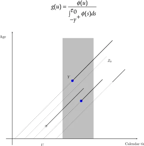
Assume that we observe all ages of onset, Y, occurring within the calendar time observation window [0; 0), cf. Figure 3 for a graphical presentation of the sampling scheme. Assume that the occurrence of births follows a Poisson process with intensity (u) for u ≤ 0, and that y+ =
sup{y: F* (y|u) < 1} exists and is finite for all u ≤ 0, i.e., y+
is the maximal observable age at onset before death. We can then normalize the birth intensity (u) to a density g
on [-y+; 0),
with associated cumulative distribution function G. In principle could well depend on covariates, but since we consider either known or constant, we will ignore this.
We will in the following assume (U1, Y1),..., (Un, Yn) to be independent and identically distributed (iid). Two crucial assumptions must be considered. First, whether or not we have calendar time stationarity with respect to age of onset, i.e.,
(S1) Age of onset is independent of time of birth, i.e.,
F(y|u) = F(y).
Secondly, knowledge about the birth process will not be available in many applications. Hence we also consider the situation with calendar time stationarity of the birth process:
(S2) Assume that the occurrence of initiating events, births, started in the distant past and that this birth rate has been stabilized. Or, quantitatively, assume that ux = inf{u: (u) > 0} is small enough so that ux ≤ -y+, and that g
is uniform on [-y+; 0).
Stationary incidence, known birth process ((S1) only)
When only (S1) holds, the joint density of the observed (u, y) can be written as follows:
≡pc(u|y)pm(y)
where pc(u|y) and pm(y) are defined by the expressions in each bracket in (3), respectively. Thus pc(u|y) can be
inter-preted as the density of birth times conditional on y being observed in [0; 0), and pm(y) as the marginal density for the observed y weighted with wi = G(0 -y) - G(-y), i.e., the probability of birth occurring within the interval [-y; 0 -y).
When g is known, then so is pc, as are the weights in pm. It is thus straightforward to compute the maximum likeli-hood estimate of F* based on the weighted observations:
The estimate thus places mass at each jump point j, where j corresponds to the observation number in the ordered set of Yi. That the estimate in (5) is the
non-g u u
s ds y
( ) ( ) ( )
= − + ∫
φ φ τ0
p u y U Y U g u I y u y
G y G y
G
( , | ) ( ) ( )
( ) ( )
{ (
− ≤ ≤ − = − ≤ ≤ −
− − − ⎡
⎣
⎢ ⎤
⎦ ⎥
×
τ τ
τ
τ
0 0
0
0−− − − ∗ ≤ +
− − − ∗
+ ∫ ⎡
⎣ ⎢ ⎢ ⎢
⎤
⎦ ⎥ ⎥
y G y f y I y y
G s G s f s ds
y
) ( )} ( ) ( )
{ (τ0 ) ( )} ( )
0 ⎥⎥
ˆ ( ) :
F y i yi ywi
wi i n
∗ = ∑ ≤ −
− = ∑
1
1 1
wj−1/
∑
w−j1Lexis diagram with observation window (gray area)
Figure 3
Lexis diagram with observation window (gray area). Dotted lines indicate lifetime without disease until age of onset (Y), or age at death (Z0), full lines lifetime with disease. Only age at onset times within the observation window are observed (blue points) in a cohort-of-cases study.
Calendar time Age
Y
Z0
Page 5 of 11 parametric maximum likelihood estimate (NPMLE)
fol-lows directly from standard results on NPMLE, see for example the paper by Turnbull [18], who covers the gen-eral case of which this is a special case. If all weights are equal, the above formula reduces to the ordinary formula for non-parametric estimation of a cdf in the uncensored case, putting mass n-1 at each jump point.
With the estimate of the conditional cdf F* it is possible to obtain an estimator of the unconditional F utilizing their relationship given in Equation (1). What we need is an estimate of ∞, which may be obtained from noting that
the occurrence rate of incident events, Itr, at any calendar
time point is given by
where the indicator function I(t - u ≤y+) is needed, since
the occurrence rate does not include those for which onset never happens, that is when y = t - u > y+or equivalently
that y = t - u = ∞. Integrating this over the observation win-dow, we find
from which it follows that
Although the estimate is intuitely attractive it is not clear whether it is the MLE. However, if we fill in the MLE of F* in Equation (12), we do obtain an estimate of ∞, since is
known and is estimated by the total number of observed incidences over the interval [0; 0). Having obtained the MLE of F* together with an estimate of ∞, we
can use Equation (1) to compute an estimate of F, the unconditional cdf of age at onset.
Stationary incidence, stationary birth process (both (S1) and (S2)) When both (S1) and (S2) hold, the marginal density of the observed y's can be further simplified by substitution of the uniform birth density in the corresponding expres-sion in Equation (3), i.e.,
Note, that here the density function of the observed y's coincides with the population density function f* of the observable onset times, Y . In the case when only age at onset distribution is of interest, and not lifetime risk, the 'usual methods' are thus applicable to the case data to esti-mate f* by putting equal weights on all observations as noted above.
If, however, we are also interested in the unconditional density, f(y), we need an estimate of ∞to be able to
pro-ceed. Above, this was obtained from our knowledge of the birth process, and in principle we could exploit this again. However, in situations where a stationary birth process is assumed, this is typically because we lack information on the birth process. Thus it may in such situations be neces-sary with alternative approaches. One obvious way to pro-ceed is the following: In the time window where information is collected on incident cases, we also collect information on deaths–either for all or a random sample– and classify them according to whether or not they had experienced disease. The relative frequency of diseased deaths will then be an estimate of ∞under stationarity
assumptions with respect to the birth process, the incidence process, and the mortality. This estimate is valid if age-spe-cific mortality is assumed stationary both among diseased and non-diseased–these strong assumptions reflect the lack of available information in such situations. With this esti-mate of ∞we may then estimate the unconditional F.
Non-stationary incidence, known birth process (Neither (S1) nor (S2)) When neither (S1) nor (S2) hold, the likelihood becomes substantially more complicated. In principle, this can be handled by introducing a parameter vector which relates the incidence density to the time of birth. The rewriting presented in Equation (4) is still valid with the modifica-tion that the density term pm(y) now depends on the parameter vector , i.e.,
I t u f t u I t u y du
t tr ( )= ( ) ( − ) ( − ≤ +) −∞
∫
φ = ∞ ∗ − −∞∫
π φ( ) (u f t u du)
t
I t dt u f t u du dt
t tr ( ) ( ) ( ) 0 0 0 0 τ τ π φ
∫
= ∞∫
∫
∗ − −∞ = ⎧⎨ − ⎩ ⎫ ⎬ ⎭ ∞ ∗ −∞∫
∫
π τ φ( ) τ ( )
max( , )
u f t u dt du
u0 0 0 = ⎧⎨ ⎩ ⎫ ⎬ ⎭ ∞ ∗ − − −∞
∫
∫
π τ φ( ) τ ( )
max( , )
u f t dt du
u u 0 0 0 = ∞
{
∗ − − ∗ −}
−∞∫
π τ0φ( )u F (τ0 u) F (max( ,0 u)) du
π∞ τ τ φ ∗τ ∗
−∞ = ⎡
{
− − −}
⎣ ⎢ ⎤ ⎦ ⎥∫
Itr( )t dt∫
( )u F ( u) F (max( , u)) du0 0
0 0
0
Itr( )t dt
0 0
τ
∫
p y y f y I y y
y
f y I y
m( )
{ /( )} ( ) ( ) /( ) ( ) ( = + + ∗ ≤ + + + ⎡ ⎣ ⎢ ⎢ ⎤ ⎦ ⎥ ⎥= ≤ ∗ τ τ τ τ 0 0 0 0
yy+)
p y G y G y f y
G s G s f s
m( | )
{ ( | ) ( | )} ( | )
{ ( | ) ( | )} ( |
θ τ θ θ θ τ θ θ = − − − ∗
− − − ∗
0
0 θθ)ds
y
0
Page 6 of 11 Unfortunately this density does not directly permit use of
the approach presented above for finding a non-paramet-ric estimate of f*(y| ), nor for finding the corresponding estimate of ∞( ).
One alternative is to set up a full likelihood by consider-ing a full parametric model of both age of onset and age of death, but we will not go into further details here and instead commend this as a topic for future research.
Ordinary non-parametric analysis
The ordinary Nelson-Aalen analysis based on observed events and time at risk is well described elsewhere, see [19] for an extensive treatment of the subject, or [20] for a more focused treatment. In short, we use age as the funda-mental time scale, and we then have delayed entry due to the fact that not all subjects are followed from birth. Rather, they enter the observation window and capture area at a certain age and are then followed until either event or censoring, whichever comes first.
We let subjects become at-risk one year after the start of the observation period if they resided in Fyn County in this period, or one year after entrance to the capture area, if they immigrated to Fyn during the study period. In both cases the one year run-in period is used to identify subjects not already in treatment (those without filled prescrip-tions in the period), as only they are at risk for becoming incident. Subjects cease to be under observation either at onset, death, emigration from Fyn, or end of follow-up, whichever comes first.
As above we require calendar time stationarity for estima-tion of F. The second assumption in this setup is that entry is independent of disease onset, i.e., age at immigration to Fyn County is not informative for the subsequent distri-bution of Y. The final assumption is that censoring is non-informative. The two latter assumptions are similar, but not identical, to the assumption of balance of migration made in the analysis of doubly truncated data. The differ-ence is, that independent delayed entry and censoring only concerns the time within the observation period. On the other hand, the balancing assumptions does not require independence, i.e., migrating subjects may well have a different morbidity than non-migrating subjects– which is indeed the case [21]–as long as the distribution of onset ages is similar among immigrating and emigrat-ing subjects.
Thus we get a non-parametric estimate of ΛY, the cumula-tive hazard for onset of disease. Similarly, a non-paramet-ric estimate of the cumulative hazard of death among
non-diseased, , can be obtained by simply exchanging
the event indicator from onset of disease to death and maintaining the at-risk time.
From ΛY and an estimate of F is given by (cf. [22] for
a theoretical discussion, while [23] gives an example of its application)
where Y is the hazard associated with ΛY, and ∞is the
life-time risk given by
As no analytic confidence intervals are available for the lifetime risk, we obtained them using bootstrap as above. This can also be applied to obtain age-specific confidence intervals for F.
Projection of incidence
Based on an estimate of F, projection of incidence is pos-sible both inside and outside the observation window by application of the formula in Equation (6), when the birth process is known and incidence is assumed station-ary. In the application studied here, the birth process is known for u ≤ 0. For u > 0 it must be projected. Hence, we carry the last observed value of the birth process forward, i.e., let (u) = (0) for u > 0.
Results and Discussion
Table 1 gives basic descriptive statististics of the studied population, as it shows the number of incidence events tabulated by gender, birth period and calendar year, which is used for estimating age-specific incidence.
Cohort-of-cases data
Complete stationarity
Although the birth process is known in our setting, we for comparison present an analysis based on assuming stationarity for the birth process, the incidence process, as well as the mortality process among treated. We first classified all deaths according to whether or not a previ-ous redemption of anti-diabetics had been observed, considering all with such a redemption to be diabetics. The lifetime risk, ∞, was for females estimated at 9.68%
(95% Confidence Interval: 9.35%; 10.02%) and for males at 10.86% (10.51%; 11.22%), where both confi-dence intervals are binomial exact. The estimated inci-dence distribution, F, stratified on gender is shown in Figure 4(a).
Az0
Az0
F y s s A s ds
I y y
Y Y z
y
( ) ( )exp[ ( )]exp[ ( )]
( )( )
= − −
+ = −
∫
+ ∞
λ
π Λ 0 0
1
π∞ = λ − −
+
∫
Y Y zy
s s A s ds
( )exp[ Λ ( )]exp[ 0( )]
Page 7 of 11 Stationarity of incidence, known birth process
When only stationarity of the incidence distribution is assumed, a non-parametric analysis based on the weighted likelihood given in Equation (4) and the estima-tor of ∞in Equation (12) can be conducted. With the
gen-der specific birth rates, we estimated gengen-der specific estimates of F*, ∞, and hence F, from the observed events
and associated ages at the events. The resulting estimates of the incidence distribution F are displayed in Figure 4(b).
We see that the incidence distribution for both genders are made up of two components: The first component is a more or less constant density for ages below 40 years (the
Table 1: Number of incidence events by gender, calendar year of event and calendar year of birth
Event year
Gender Birth 1993 1994 1995 1996 1997 1998 1999 2000 2001 2002 2003
Females -1909 60 24 30 22 7 19 9 7 6 4 4
1910-9 103 79 74 101 81 69 66 58 65 51 47
1920-9 110 123 99 122 98 112 118 109 106 119 118
1930-9 65 86 78 86 96 82 96 108 111 132 140
1940-9 51 51 55 70 65 64 88 100 115 117 137
1950-9 41 31 32 26 32 30 38 48 51 64 70
1960-9 18 18 13 20 8 18 28 29 30 34 48
1970-9 17 10 9 6 13 5 9 9 18 19 34
1980-9 4 3 24 5 6 8 7 9 5 11
1990- 4 6 3 3 5 7 10 10
Males -1909 29 19 18 8 7 7 4 2 2 2
1910-9 94 80 68 71 65 58 42 45 37 21 28
1920-9 126 145 106 118 96 116 99 93 82 123 123
1930-9 107 95 114 132 126 119 131 156 143 126 174
1940-9 104 102 83 102 111 129 140 166 183 191 214
1950-9 49 52 38 52 42 77 65 70 77 106 113
1960-9 16 19 19 21 27 23 28 29 41 55 53
1970-9 12 11 17 8 5 7 10 9 15 14 12
1980-9 8 2 3 28 6 2 7 12 12 12 10
1990- 5 3 2 6 7 8 9 5
Number of incidence events by gender, calendar year of event and calender year of birth.
Estimated incidence distribution F for pharmacological treatment with any anti-diabetic drug with respect to age, and stratified
on gender
Figure 4
Estimated incidence distribution F for pharmacological treatment with any anti-diabetic drug with respect to age, and stratified on gender.
0
.05
.1
.15
F
0 20 40 60 80 100
age
Females Males
(a) Stationary birth and incidence process
0
.05
.1
.15
F
0 20 40 60 80 100
age
Females Males
Page 8 of 11 linear part in F), whereas the second is a much higher,
uni-modal density for ages above 40 years which vanishes for ages above 80 (the sigmoid shaped part of F). For females the lifetime risk, ∞, was estimated at 13.77% (13.74%;
13.81%), for males at 15.61% (15.58%; 15.65%). Both confidence intervals are computed using bootstrap with a thousand replications. The confidence intervals are very narrow which reflects the high statistical efficiency of the weighted likelihood approach–which in turn partly comes from the strong assumption of stationarity. As birth counts are assumed known, this too contributes to the narrow confidence intervals, although to a lesser degree.
The shape of F is quite similar to the unweighted estimate, whereas the estimated lifetime risks are substantially higher than those estimated above. The major explana-tion is of course lack of staexplana-tionarity of the true lifetime risk and/or the disease duration: The estimate of ∞based on
disease status among observed deaths takes most of its information from the older cohorts as they are the ones with high mortality. If the older cohorts had lower life-time risk and/or previously had relatively higher mortality among diseased compared to non-diseased (both of these scenarios are very realistic, but contrary to assumptions of the previous analysis), this will result in a decreased esti-mate of ∞. This would be amplified if older cohorts are
larger than younger cohorts, as is indeed the case here, cf. Figure 2.
Contrastingly, when indirectly estimating ∞ based on
weighting with the birth process, the estimate can be viewed as a weighted average of ∞over the entire interval
for the birth process [-y+; 0 -y).
Projection of diabetes incidence
In the completely stationary situation, where (S1) and (S2) are both assumed to hold, the projected annual inci-dence is a constant number equaling the lifetime risk mul-tiplied by the annual number of births. As the annual number of births are usually not observable in such set-tings, an alternative is needed. In the spirit of estimating
∞from the treatment status among deaths, one could take
the total annual number of deaths as an estimate of the number of births. The reasoning for this is that if the pop-ulation is in a completely stationary state, the annual number of deaths must on average equal the average annual number of births. In our setting the observed numbers of deaths over the 11 year period are 29,871 for females and 29,816 for males yielding projected, annual incidences of 262.8 for females and 294.3 for males. In Figure 5 the incidence is projected based on the weighted, non-parametric estimate of F obtained above, i.e., with known birth intensity and stationary incidence. All annual birth counts after 2003 are set to the number of
births observed in 2003. Note, that the observed inci-dence strongly suggests a departure from stationarity, and so future actual incidences are likely to be higher than those projected from a stationarity assumption. The pro-jected incidences show a small but persistent decline for 2004–2013 due to declining birth rates in the last half of the twentieth century. The general level is much higher than above, reflecting the higher estimate of ∞obtained
from using the known birth distribution, but correspond well with observed incidences.
Ideally, projections should be accompanied by confi-dence intervals, but we have been unable to compute them. While in principle some variant of bootstrap might be employed, this is numerically very demanding as the entire cdf of age-specific incidence must be bootstrapped. Judged from the conifdence intervals of the lifetime risks, the confidence intervals of the projections will be very small, reflecting both high efficiency of the method, as well as its strong assumptions.
Ordinary non-parametric analysis
The gender specific estimates of F are shown in Figure 6. The shape of the estimated cdf is very similar to the one obtained above using a known birth process for weight-ing. The estimated lifetime risks are 15.65% (15.14; 16.16) for females, and 17.91% (17.38; 18.44) for males, where confidence intervals were found from bootstrap with 1,000 replications. This is somewhat higher than when analyzing data as doubly truncated. The explana-tion is that mortality has generally declined substantially over the past century, and hence an estimate based on the mortality rates observed within the observation window
Projected and observed annual numbers of incident events in the county of Fyn based on an assumption of a stationary
incidence and using a weighted, non-parametric estimate of F
Figure 5
Projected and observed annual numbers of incident events in the county of Fyn based on an assumption of a stationary incidence and using a weighted, non-parametric estimate of F.
0
200
400
600
800
1993 1995 1997 1999 2001 2003 2005 2007 2009 2011 2013 year
Page 9 of 11 leads to a higher risk of diabetes onset prior to death than
an estimate which implicitly accounts for past mortality.
Projection of diabetes incidence
Projections are obtained as above–except that the ordi-nary non-parametric estimate of F is used–and results are shown in Figure 7. Due to the elevated lifetime risk the projected incidences are now higher–also too high com-pared to observed incidences. Also for this projection we have been unable to provide confidence intervals for the same reasons as above.
Conclusion
In this paper we have developed and implemented meth-ods for estimating and projecting incidence, as well as the lifetime risk of a disease based on observation of incident events in an observation window, i.e., what we termed cohort-of-cases data. The developed methodology yields non-parametric estimates comparable to those of a stand-ard Nelson-Aalen analysis based on independent delayed entry, but it gives slightly better projections of incidence due to its implicit accounting for the unobserved mortal-ity among untreated in the past.
In its simplest form–i.e., assuming both a stationary birth process and incidence–a simple non-parametric estimate of the age of onset distribution is obtained. When alterna-tively the birth process is considered known, this is taken into account by a weighted, non-parametric estimate with weights based on the relative sizes of the relevant birth cohorts. Both approaches directly provide estimates of age-specific incidence as well as of lifetime risk, which are of considerable public health interest. Due to the
rela-tively fast computational procedures developed, confi-dence intervals for the lifetime risk could be obtained from direct application of bootstrap methodology. We were however unable to provide confidence intervals for projection of incidence.
As stated by Narayan et al. in 2003, lifetime risk of diabe-tes appears not to have been estimated prior to their paper [8], and only one subsequent paper have reported comparable estimates of lifetime risk [24]. The directly comparable estimates for the US population found in [8] are substantially higher (39% for females, 33% for males) than ours (14% for females, 16% for males). The two major reasons for the difference is a generally lower diabetes incidence in Denmark [4], as well as the fact that our estimates only pertain to pharmacologically treated diabetes. It would however be interesting to explore if part of the difference is due to their use of the traditional method, as the traditional method in our material leads to an elevated estimate of lifetime risk of 16% for females and 18% for males. It is further interesting that the gen-der differences are in opposite directions in the two countries.
Several papers have used estimates of incidence to project the future burden of diabetes, most prominently [2,5,6]. For all three, it would be interesting to re-analyze their data using our developed method for cohort-of-cases data, if possible, to see if a similar discrepancy exist between the two analytical methods as we have found, where the traditional method lead to an inflated projec-tion of the number of incident events of diabetes, when compared to the observed count.
Estimated incidence distribution F for pharmacological treat-ment with any anti-diabetic drug with respect to age, and stratified on gender
Figure 6
Estimated incidence distribution F for pharmacological treat-ment with any anti-diabetic drug with respect to age, and stratified on gender. Ordinary non-parametric estimate with independent delayed entry.
0
.05
.1
.15
.2
F
0 20 40 60 80 100
Age
Females Males
Projected and observed annual numbers of incident events in the county of Fyn based on the ordinary non-parametric
esti-mate of F with independent delayed entry
Figure 7
Projected and observed annual numbers of incident events in the county of Fyn based on the ordinary non-parametric esti-mate of F with independent delayed entry.
0
200
400
600
800
1993 1995 1997 1999 2001 2003 2005 2007 2009 2011 2013 year
Page 10 of 11 For the theoretical developments, assumptions (S1) and
(S2) have been crucial, but from an applied perspective the assumptions are very restrictive. In our application concerning diabetes, the assumptions are likely not satis-fied, as it is questionable that both age-specific incidence and age-specific mortality among diabetics have been constant since 1900–rather, changes in incidence due to altered lifestyle, and changes in mortality due to improved treatment and general health are reasonable. Indeed, it is known that within the observation window of 1993 and 2003, statistically significant trends exist for both quanti-ties [4]. Yet the predictions based on the developed model are at least as good as those based on the ordinary non-parametric method, showing the potential of the devel-oped model. More work on relaxing the assumptions is however mandated before the model can be used more generally.
Although we in principle showed how the stationarity assumption could be relaxed by formulating a full, para-metric likelihood, we did not give a detailed analysis of this situation due to its complexity. Also, the data consid-ered in this paper are rather limited since, first, the obser-vation window is short compared to typical disease duration, and second, no information is available on age of onset outside the observation window. As a result, we have been unable to allow for trends in incidence and mortality, the absence of which must be considered unre-alistic. In some epidemiological settings it will, however, be possible to obtain data on age of onset for subjects prevalent at start of the time window or for diseased sub-jects dying in the observation window [25]. While such information is valuable and needs to be incorporated in the analysis to allow relaxation of assumptions, it requires knowledge about the past mortality among diabetics. In contrast, we have tried to develop a methodology that only rely on observation of incident events and past birth rates, which are often easier to obtain. There is, however, a need for further research on the applicability and exten-sions of the method before its potential can be more clearly appreciated.
Competing interests
The author(s) declare that they have no competing inter-ests.
Authors' contributions
HS had the original idea for the study, carried out all anal-yses and drafted the original and revised manuscripts with substantial input from MCW. The planning of analyses and interpretation of the data was the joint product of dis-cussions between MCW and HS. Both authors have seen and approved the final version.
References
1. Mokdad A, Bowman B, Ford E, Vinicor F, Marks J, Koplan J: The con-tinuing epidemics of obesity and diabetes in the United States. JAMA 2001, 286:1195-200.
2. Honeycutt AA, Boyle JP, Broglio KR, Thompson TJ, Hoerger TJ, Geiss LS, Narayan KMV: A dynamic Markov model for forecasting diabetes prevalence in the United States through 2050.
Health Care Manag Sci 2003, 6(3):155-164.
3. Wild S, Roglic G, Green A, Sicree R, King H: Global prevalence of diabetes: estimates for the year 2000 and projections for 2030. Diabetes Care 2004, 27(5):1047-53.
4. Støvring H, Andersen M, Beck-Nielsen H, Green A, Vach W: Count-ing drugs to understand the disease: The case ofmeasurCount-ing the diabetes epidemic. Popul Health Metr 2007, 5:2.
5. Narayan KMV, Boyle JP, Geiss LS, Saaddine JB, Thompson TJ: Impact of recent increase in incidence on future diabetes burden: U.S., 2005–2050. Diabetes Care 2006, 29(9):2114-2116.
6. Evans JMM, Barnett KN, Ogston SA, Morris AD: Increasing preva-lence of type 2 diabetes in a Scottish population: effect of increasing incidence or decreasing mortality? Diabetologia
2007, 50(4):729-732.
7. Fox CS, Pencina MJ, Meigs JB, Vasan RS, Levitzky YS, D'Agostino RB:
Trends in the incidence of type 2 diabetes mellitus from the 1970s to the 1990s: the Framingham Heart Study. Circulation
2006, 113(25):2914-2918.
8. Narayan KMV, Boyle JP, Thompson TJ, Sorensen SW, Williamson DF:
Lifetime risk for diabetes mellitus in the United States. JAMA
2003, 290(14):1884-1890.
9. Harris M, Flegal K, Cowie C, Eberhardt M, Goldstein D, Little R, Wiedmeyer H, Byrd-Holt D: Prevalence of diabetes, impaired fasting glucose, and impaired glucose tolerance in U.S. adults. The Third National Health and Nutrition Examina-tion Survey, 1988–1994. Diabetes Care 1998, 21(4):518-24. 10. Prentice RL: A Case-Cohort Design for Epidemiologic Cohort
Studies and Disease Prevention Trials. Biometrika 1986,
73:1-11.
11. Mantel N: Synthetic retrospective studies and related topics.
Biometrics 1973, 29(3):479-86.
12. Prentice RL, Breslow NE: Retrospective Studies and Failure Time Models. Biometrika 1978, 65(1153-158 [http://links.jstor.org/
sici?sici=0006- 3444%28197804%2965%3A1%3C153%3ARSAFTM%3E2.0.CO%3B2-E].
13. Oakes D: Survival times: aspects of partial likelihood. Internat Statist Rev 1981, 49(3):235-264. With discussion and a reply by the author
14. Thomas DC: General Relative-Risk Models for Survival Time and Matched Case-Control Analysis. Biometrics 1981,
37(4673-686 [http://links.jstor.org/sici?sici=0006-341X%28198112%2937%3A4%3C673%3AGRMFST%3E2.0.CO%3B2 -V].
15. Lubin J, Gail M: Biased selection of controls for case-control analyses of cohort studies. Biometrics 1984, 40:63-75.
16. The WHO Collaborating Centre for Drug Statistics Methodology:
ATC index with DDDs and Guidelines for ATC classification and DDD assignment. Oslo 2001.
17. Støvring H, Andersen M, Beck-Nielsen H, Green A, Vach W: Rising prevalence of diabetes: evidence from a Danish pharmaco-epidemiological database. Lancet 2003, 362(9383):537-8. 18. Turnbull BW: The empirical distribution function with
arbi-trarily grouped, censored and truncated data. J R Statist Soc A
1976, 38(3):290-295.
19. Andersen PK, Borgan O, Gill RD, Keiding N: Statistical models based on counting processes New York: Springer-Verlag; 1997. Corrected second printing
20. Keiding N: Independent delayed entry. In Survival Analysis: State of the Art Edited by: Klein JP, Goel PK. Kluwer Academic Publishers; 1992:309-326.
21. Støvring H: Selection bias due to immigration in pharmacoep-idemiologic studies. Pharmacoepidemiol Drug Saf 2007,
16(6):681-686.
22. Keiding N: Age-specific Incidence and Prevalence: a Statistical Perspective. J R Statist Soc A 1991, 154(3):371-412.
Publish with BioMed Central and every scientist can read your work free of charge
"BioMed Central will be the most significant development for disseminating the results of biomedical researc h in our lifetime."
Sir Paul Nurse, Cancer Research UK
Your research papers will be:
available free of charge to the entire biomedical community peer reviewed and published immediately upon acceptance cited in PubMed and archived on PubMed Central yours — you keep the copyright
Submit your manuscript here:
http://www.biomedcentral.com/info/publishing_adv.asp
BioMedcentral
Page 11 of 11
of Forensic Medicine following violent victimisation? Injury
2006, 39(1):121-127.
24. Narayan KMV, Boyle JP, Thompson TJ, Gregg EW, Williamson DF:
Effect of BMI on lifetime risk for diabetes in the U.S. Diabetes Care 2007, 30(6):1562-1566.
25. Keiding N, Holst C, Green A: Retrospective estimation of diabe-tes incidence from information in a prevalent population and historical mortality. Am J Epidemiol 1989, 130(3):588-600.
Pre-publication history
The pre-publication history for this paper can be accessed here:
http://www.biomedcentral.com/1471-2288/7/53/prepub
Publish with BioMed Central and every scientist can read your work free of charge
"BioMed Central will be the most significant development for disseminating the results of biomedical researc h in our lifetime."
Sir Paul Nurse, Cancer Research UK
Your research papers will be:
available free of charge to the entire biomedical community peer reviewed and published immediately upon acceptance cited in PubMed and archived on PubMed Central yours — you keep the copyright
Submit your manuscript here:
http://www.biomedcentral.com/info/publishing_adv.asp