of human chest and phantom tank via
sinc-convolution algorithm
Abbasi and Naghsh-Nilchi
R E S E A R C H
Open Access
Precise two-dimensional D-bar reconstructions
of human chest and phantom tank via
sinc-convolution algorithm
Mahdi Abbasi
*and Ahmad-Reza Naghsh-Nilchi
* Correspondence:m_abbasi@eng. ui.ac.ir
Department of Computer Engineering, Engineering Faculty, University of Isfahan, Isfahan, Iran
Abstract
Background:Electrical Impedance Tomography (EIT) is used as a fast clinical imaging technique for monitoring the health of the human organs such as lungs, heart, brain and breast. Each practical EIT reconstruction algorithm should be efficient enough in terms of convergence rate, and accuracy. The main objective of this study is to investigate the feasibility of precise empirical conductivity imaging using a sinc-convolution algorithm in D-bar framework.
Methods:At the first step, synthetic and experimental data were used to compute an intermediate object named scattering transform. Next, this object was used in a two-dimensional integral equation which was precisely and rapidly solved via sinc-convolution algorithm to find the square root of the conductivity for each pixel of image. For the purpose of comparison, multigrid and NOSER algorithms were implemented under a similar setting. Quality of reconstructions of synthetic models was tested against GREIT approved quality measures. To validate the simulation results, reconstructions of a phantom chest and a human lung were used.
Results:Evaluation of synthetic reconstructions shows that the quality of sinc-convolution reconstructions is considerably better than that of each of its competitors in terms of amplitude response, position error, ringing, resolution and shape-deformation. In addition, the results confirm near-exponential and linear convergence rates for sinc-convolution and multigrid, respectively. Moreover, the least degree of relative errors and the most degree of truth were found in
sinc-convolution reconstructions from experimental phantom data. Reconstructions of clinical lung data show that the related physiological effect is well recovered by sinc-convolution algorithm.
Conclusions:Parametric evaluation demonstrates the efficiency of sinc-convolution to reconstruct accurate conductivity images from experimental data. Excellent results in phantom and clinical reconstructions using sinc-convolution support parametric assessment results and suggest the sinc-convolution to be used for precise clinical EIT applications.
Keywords:EIT, D-bar, Sinc-convolution, Accuracy measures, Chest phantom, Human chest
Background
Electrical impedance tomography is a new non-invasive imaging technique in which the conductivity distribution inside a body is reconstructed via knowledge of injected current patterns and resulted induced voltages through finite number of electrodes placed on its surface [1]. This modality has many medical applications including monitoring heart and lung functions [2,3], breast cancer detection [4] and diagnosis of pulmonary edema and diagnosis of the pulmonary embolus [5].
Reconstructing the conductivity images in EIT involves solving forward and inverse problems [1]. The solution of the forward problem is the potential distribution inside the body given the map of conductivity distribution. The inverse problem is to find the unknown conductivity map inside the body using finite sets of injected current patterns and measured voltages on the electrodes surrounding the body.
Algorithms for solving the forward problem of EIT use Finite Element Methods (FEM), Boundary Element Methods (BEM) and Finite Difference Methods (FDM)[1]. Existing approaches for solving the inverse problem of EIT include:
1. Linearized iterative methods such as Calderon’s method [6], back-projection [7,8] and NOSER [9], which are not able to reconstruct conductivity distributions with high variations [10].
2. Non-linear iterative methods such as equation error formulation [11], output least square [12], statistical inversion [13] and Newton–Raphson methods [14], which are accurate but suffer from the low convergence rate and high computational complexity [10]. 3. Layer stripping methods [15] which are sensitive to noise and are weak in
reconstruction of non-symmetric conductivities [10].
4. Direct algorithms such as D-bar [16] and Block method [17] which solve the full nonlinear inverse problem without any iteration in the conductivity domain and do not require any intermediate estimation of the conductivity from a forward model. Block method gains considerably from the homogeneity of conductivity distribution for particles inside each block of the body [17]. The problem of high computational burden faced in this method can be resolved by the method of modified equations [18]. Recently, a non-iterative linear inverse solution is introduced in [19] that raises the efficiency of this method via reduction in its computational complexity.
D-bar method is a new direct methodology, which was firstly introduced in the constructive proof of Nachman [16]. This method uses the properties of the D-bar operator of inverse scattering [20] to solve the full non-linear inverse conductivity problem on the planar domains with two degrees of derivatives. An overview of this method is provided in the following section. The reader can refer to [16] for more details. Note that, the quality of the reconstructed conductivity images by the D-bar method is highly affected by approxi-mate numerical solution to a weakly singular integral equation, named D-bar [21-23].
The complexity and high rates of error of PI-based methods inspired the adaptation of MG methods [25] for solving D-bar integral equation. Although MG methods solve D-bar integral equation with a remarkable speed and decrease the computational burden fromO
(N6) toO(N4logN) incorporating Fast Fourier Transform (FFT), the convergence rate of these methods may not reach ultra-linear levels [22]. Recently, Mueller [26] has employed MG solution of D-bar equation to reconstruct physical tank and human chest conductivity images. In addition to the presence of visual artifacts such as blurring, the position, size and orientation of the organs are not correctly reconstructed by MG.
These considerable drawbacks in aforementioned methods motivated us to present an ef-fective computational algorithm based on sinc-convolution method to solve D-bar equation with higher accuracy and lower computational burden [27]. But, for an EIT algorithm to be practically used, some numerical and experimental proficiency tests are required to show its actual efficiency [10].
The aim of this study is to assess the feasibility of empirical conductivity image reconstruction via sinc-convolution algorithm in the D-bar framework of EIT. A regular EIT algorithm evaluation requires a standard test methodology which is followed by some experimental reconstructions. In this study, the approved parametric test methodology of [2] is used to evaluate sinc-convolution algorithm based on the reconstructions of a specific synthetic model. The employed scenario is described subsequently. After parametric evaluation of the sinc-convolution, two sets of boundary data are used to qualitatively asses the reconstructions of sinc-convolution. Indeed, these experiments validate the parametric evaluations and show real potency of the sinc-convolution for clinical EIT. For the purpose of comparison, two other algorithms including MG and NOSER are implemented.
The paper is organized as follows. In the immediately following section, steps of the D-bar algorithm of Nachman are reviewed. Next, the sinc–convolution algorithm for solving D-bar integral equation is described. After establishing synthetic models and explaining phantom and clinical measurements, computations of performance figures are described. The parametric evaluation results of sinc-convolution, MG and NOSER are followed by their experimental reconstructions of a phantom tank and a human lung data.
Methods
The EIT problem on a two-dimensional simply connected region Ωis modeled by the generalized Laplace equation as
r:ðγð Þrx u xð ÞÞ ¼0; x¼ðx1;x2Þ 2Ω; ð1Þ
where γ(.) andu(.) represent the conductivity of the domain and the electric potential, respectively. The Dirichlet boundary condition
u xð Þ ¼f xð Þ; x¼ðx1;x2Þ 2@Ω; ð2Þ
represents the known voltage distribution, f, on the boundary of the Ω, resulted from injecting a known current density, g, on the boundary that corresponds to Neumann boundary condition
g xð Þ ¼γð Þx @u
Here, v denotes the outward normal on the boundary @Ω. The voltage-to-current map takes the given voltage distribution fon the boundary to current density distribu-tion g. This mapping is also called Dirichlet-to-Neumann mapping and is denoted by
Λγin EIT literature [10].
Actually, the inverse conductivity problem as stated firstly by Calderon [6] is to uniquely determine the unknown conductivity distribution γ from the knowledge of
Λγ. There have been extensive efforts to find and prove the uniqueness of the solution to this problem including the work of Nachman [16], Brown-Uhlmann [28] and recently Astala [29] for two-dimensional inverse conductivity problem. All of these researches are based on the D-bar method of inverse scattering [30].
Methods: D-bar method of EIT
The essence of the D-bar method of EIT is to transform the conductivity equation to Schrödinger equation and use the D-bar approach of inverse scattering to solve the resulting equation. For more details about the theory, the reader is referred to [16]. Here, we only review D-bar equations from the constructive proof of Nachman [16] for solving inverse conductivity problem on a simply connected two-dimensional region with two derivatives.
Change of the variable Ψ=γ1/2μand q=Δγ1/2/γ1/2and assuming that γ is a constant γbestin the neighborhood of the boundary transforms the conductivity equation (1) to
Schrödinger equation in wholeR2[16] Δþq
ð ÞΨðx;kÞ ¼0; x2R2: ð4Þ
Note that, in the D-bar method a point x=(x1,x2)2Ω may be identified as a point x=x1+ix2where i2=-1 in complex plane. Also the complex parameter k=k1+ik22Cmay be identified as a point k=(k1,k2)2R2. Using the assumption thatγis a constant,γbestin
the neighborhood of the boundary or equivalently q=0 outside the boundary, leads to another Schrödinger equation [16]
Δþq
ð Þγ1=2ð Þ ¼x 0; x2R2: ð5Þ
The key idea behind the proof of Nachman is that since two equations (4), (5) have same compact potentials q, the unique solution of equation (4) can be used to find the unique solution to equation (5). That isγ1/2(x) =ψ(x,k),for x2R2. The unique solution ψ(x,k) to equation (4) is called exponentially growing solution which was first intro-duced by Faddeev [31]. This solution is asymptotic to eikx for large |x| or large |k|. Defining the function [16]
μðx;kÞ ¼eikxψðx;kÞ; ð6Þ
which is asymptotic to 1 and considering aforementioned key idea in the Nachman’s proof [16], the conductivityγ(x) can be computed as
γð Þ ¼x lim k!0μðx;kÞ
2
In the constructive proof of Nachman, an intermediate none-physical function named scattering transform ofq(x) is defined as [16]
t kð Þ ¼
Z
R2
eikxq xð Þψðx;kÞdx; ð8Þ which plays an important role in relating the measurement data and the conductivity distribution γ(x). Note that, in equation (8), k¯ and x¯ are respectively the complex conjugates of k and x. By simplifying the equation (8), the scattering transform is related to the Dirichlet-to-Neumann map using the formula [16]
t kð Þ ¼γbest
Z
@Ω
eikx ΛγΛ1
ψð Þ:;k dσð Þx : ð9Þ
Here, Λγ denotes the voltage-to-current density map when Ω has the conductivity distribution γand Λ1denotes the voltage-to-current density map for homogenous con-ductivityγ= 1. Using the large |x| asymptotic behaviorψ(x,k)|@Ωeikx, an approximation
to scattering transform of equation (9), namelytexp(k) is introduced [23] in the form
texpð Þ ¼k γbest
Z
@Ω
eikx ΛγΛ1
eikxdσð Þx : ð10Þ
As shown in [32], as a regularization, the approximate computation of scattering transform texp(k) should be restricted to a disk of radius R in the complex plane and should be set to zero outside the disk. Therefore, the approximate scattering transform
tRexp(k)is defined as a compactly support function by [23]
tRexpð Þ ¼k γbest
R @Ω
eikx Λ γΛ1
eikxdσð Þx; j jk ≤R:
0; j jk >R
(
ð11Þ
The tRexpð Þk approximation is used in some D-bar reconstructions using numerically
simulated data [23,24,33], experimentally collected data on phantom tank [21] and human chest data [34].
It is shown by Nachman [16] that the connection between the scattering transform and theμ(x,k) is provided by D-bar equation as
@kμðx;kÞ ¼ 1 4πkt
exp
R ð Þk ekð Þx μðx;kÞ
; ð12Þ
where ekð Þ ¼x exp i xkþxk
¼ expð2i xð 1k1þx2k2Þ:
This equation has a unique solution that satisfies two-dimensional singular D-bar integral equation [16]
μð Þ ¼x;s 1þ 1 4π
Z
R2
tRexpð Þk sk
ð Þkekð Þx
μðx;kÞ
dk: ð13Þ
In [27] a novel sinc-convolution algorithm is introduced for solving D-bar equation of (13). This sinc-convolution algorithm is based on using collocation to replace two-dimensional D-bar convolution equation by a system of algebraic equations. Separation of variables in the proposed method allows elimination of the formulation of huge full matrices and therefore reduces the computational complexity drastically. In addition,
Methods: numerical solution of D-bar equation via sinc-convolution
Here, the iterative sinc-convolution algorithm to solve the D-bar integral equation (13) is reviewed. The computational steps of sinc-convolution algorithm are enlisted in Table 1. As a matter of fact, the sinc-convolution method is used to replace the integral equation (13) by a system of algebraic equations.
Recall from the previous section that the support of scattering transform may be embedded in a disk of radius R. In the first step of the sinc-convolution algorithm the required bounds of two-dimensional convolution integral are determined as [−2R, 2R] × [−2R, 2R]. This provides the required knowledge to define the sinc-points via definition of region-related mapping functions in the next step of algorithm. In the second step of algorithm, the two-dimensional convolution integral in the right-hand-side of equation (13) is decomposed into four two-dimensional convolution integralsri,i= 1, .., 4.
Third step of the sinc-convolution algorithm forms the required matrices for iterative solution of the D-bar equation. In the fourth step, a special“Laplace transform”of the kernel of the D-bar equation should be computed. This transform is used in the iterative computations of the sinc-convolution [27].
As clearly indicated in the fifth step of the sinc-convolution algorithm in Table 1, the separation-of-variables procedure of Table 2 is used to compute all four two-dimensional convolution integrals ri,i= 1, .., 4. This feature of the sinc-convolution allows computing a
Table 1 The sinc-convolution algorithm
Step Operation
1 Specify the bounds of D-bar integral equation
μðx;kÞ ¼1þr kð Þπ ;wherer kð Þ ¼ R 2R 2R R 2R 2R texp
R ekð Þx 4k sðkÞ
μðx;kÞ
dk1dk2;k¼k1þik22C;k6¼0:
2
1. Decompose convolution integral r¼P4
i¼1 ri
2. Define mapping functionsφ1ð Þ ¼zl φ2ð Þ ¼zl φð Þ ¼zl ln z2lRþ2zRl
;l¼ M;. . .;N:
3. Compute sinc points zl¼φ1ð Þ ¼lh
2Rð1þelhÞ 1þelh
ð Þ ;l¼ M;. . .;N:
4. Compute derivative of the mapping functions at sinc pointsφ0ð Þ ¼zl 2Rþz4R
l
ð Þðzl2RÞ 3
Use sinc matricesI1
mið Þ ¼s;t R st
0 sinð Þπz
πz dzþ0:5; for s;t¼ M; ::;N;
A1¼hI1
mD
1 φ0ð Þzl
¼X1S1X1 1 ;
A2¼h I1
m T
D 1
φ0ð Þzl
¼X2S2X1 2 :
4 Compute the special“Laplace Transform”of the convolution kernelg kð Þ ¼1
k;k¼k1þik22C
G uð ;vÞ ¼ Z1
0 Z1
0
g k1ð ;k2Þe
k1 uþ k2 v dk1dk2
¼ πv π
2 v u þln
v u
1þ v u
2 þi
u π
π 2
u v þln
u v
1þ u v
2 ; where Re u v >0;Re
v u >0:
5 Iteratively
1.Compute eachri;i¼1; ::;4;using the separation-of-variables procedure of Table2.
2.Solve equationμð Þ ¼k 1þ1
two-dimensional convolution integral ri,i= 1, .., 4, by only some one-dimensional vector
operations.
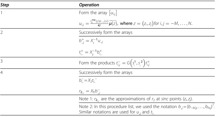
Here, the algorithm for computingr2is summarized and listed in Table 2. Note that, in the sinc-convolution method, as fully explained in [27], the separation of the variables of all four two-dimensional integrals in the D-bar equation may be done analogously.
Sum of these integrals reassembles the r matrix in the right-hand-side of the discrete-form D-bar equation as:
μ¼1þ1
πr: ð14Þ
Here, μ= [μij]m×mfor m=M+N+ 1 with elementsμij=μ(zi,zj). That is, the elements
of this matrix are actually the values of the solution at sinc points. The 1on the right hand side of the equation (14) denotes a vector of size m2of 1’s. The equation (14) is solved by means of an iterative solver such as GMRES [35]. It is worth noting that since GMRES can only work with real-linear operators, the real and imaginary parts of the solution matrix,μ, must be kept separate [35].
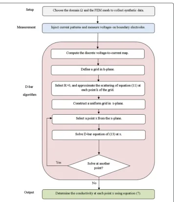
Methods: computational steps of D-bar reconstruction
To use both of the aforementioned datasets in the D-bar algorithm, the steps of the flowchart in Figure 1 must be followed. According to that flowchart, one may need to approximately compute the discrete form of the voltage-to-current map from the finite measurement data and then approximately compute the scattering transforms.
Computing the discrete dirichlet-to-Neumann map
In this study, known patterns of current are injected through the electrodes surrounding the body and the induced voltages on the same set of the electrodes are measured. Hence, the primary step in reconstruction is to construct the discrete version of the voltage-to-current density map in the form of a matrix from the injected voltage-to-current and measured volt-age values. In this study, the method introduced by Isaacson in section 3 of [21] to Table 2 Computing r2using the separation of variables procedure
Step Operation
1 Form the array ui;j
ui;j¼t exp
R ð Þzezð Þx 4z μð Þz
;wherez¼ zi;zj
for i;j¼ M;. . .;N:
2 Successively form the arrays
bþ:;j¼X1
1 u:;j
ti;:þ¼X1
2 b
þ
i;:
3 Form the productst
i;j¼G s1i;s 2 j
tþi;j
4 Successively form the arrays
bi−,.=X2ti,.−
r2i;j ¼X1b:;j
Note 1:r2i;jare the approximations ofr2atsincpoints (zi,zj).
Note 2: In this procedure list, we used the notationb.,j= (b−M,j,. . .,bN,j) T
construct the voltage-to-current density matrix from the boundary measurements on a phantom chest is followed. This computational method is used in all experimental D-bar reconstructions such as [26,34,36]. The reader is referred to [21] for analytical derivation of this approximation. Here, we briefly summarize that to fix the notations. Let
L = the number of electrodes
A = the area of an electrode, which is uniform in this study Δθ= the angle in radian between each electrode
r = radius of the circular domain (in this study the radius of the tank).
In our study, L-1 trigonometric current patterns with amplitude M are used. The j-th current pattern on thel-th electrode is defined by [21]
Tlj¼
Mcosð Þjθl ; j¼1;. . .;
L
21
Mcosð Þπl ; j¼L
2
Msin jL
2
θl
; j¼L
2þ1;. . .;L1
: 8 > > > > > < > > > > > :
ð15Þ
Let tljdenote the vector of normalized currents tj¼ T j
∥Tj∥, where ∥Tj∥¼
ffiffiffiffiffiffiffiffiffiffiffiffiffiffiffiffiffiffi PL i¼1
Tlj 2
r
.
Also let Vljdenote the voltage measured on the l-th electrode corresponding to j-th
current patternTjand normalized so thatPL i¼1
Vlj¼0;j¼1;. . .;L1. Then, the voltages vjthat would result from the normalized current patterns are given byvj¼ Vj
∥Tj∥.
Let the (u(.),w(.))Ldenote the discrete inner product defined by
uð Þ: ;wð Þ:
ð ÞL¼
XL
1
uð Þθl
wð Þθl : ð16Þ Then the entries of the discrete Neumann-to-Dirichlet mapRγ,rare approximated by [21]
Rγ;rðm;nÞ ¼
tml A;v
n l
L
;where m;n¼1;. . .;L1: ð17Þ Finally, by computing [21]
Lγ;r¼Rγ;r1; ð18Þ one can obtain the discrete approximation of the Dirichlet-to-Neumann mapΛγ. Using
the analytical method introduced in [21], the discrete current-to-voltage map R1,r is
approximated by the diagonal matrix
R1;rðm;nÞ ¼ 1
A
1
m; m¼n and m;n≤L=2:
1
mL=2; m¼n and m;n>L=2 0; otherwise:
: 8 > > > < > > > :
ð19Þ Similarly, the discrete approximation of theΛ1is obtained by [21]
L1;r¼R1;r1: ð20Þ Finally, computing [21]
δLγ;r¼Lγ;rL1;r; ð21Þ
gives the discrete approximation to (Λγ−Λ1) .
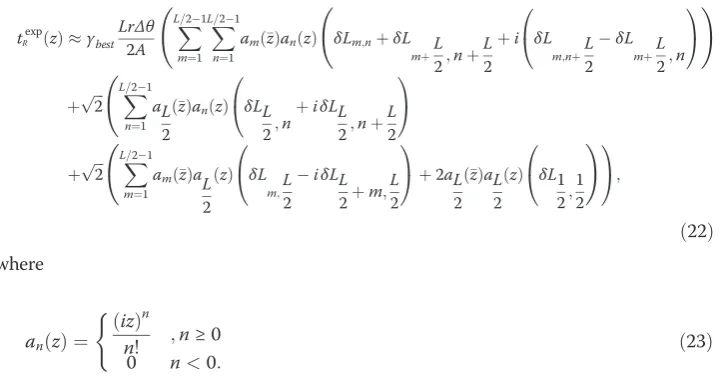
Computing the scattering transform tRexpð Þk
The series formulation for scattering transformtRexp, firstly derived by Isaacson in [21] and
tRexpð Þ z γbest LrΔθ
2A X L=21
m¼1
X L=21
n¼1
amð Þz anð Þz δLm;nþδL mþL
2;nþ L 2
þi δL m;nþL
2 δL
mþL
2;n 0
@
1 A
!
þpffiffiffi2 X L=21
n¼1aL
2 z
ð Þanð Þz δLL 2;n
þiδLL 2;nþ
L 2 0 @ 1 A
þpffiffiffi2 X L=21
m¼1
amð Þz a L 2 z ð Þ δL
m;L 2
iδLL 2þm;
L 2 0
@
1 Aþ2aL
2 z ð ÞaL
2 z ð Þ δL1
2; 1 2 ! 0 @ 1 A; ð22Þ where
anð Þ ¼z
iz
ð Þn
n! ;n≥0
0 n<0: (
ð23Þ
The method of computingγbest, the best constant conductivity fit to measured data,
is found in Appendix A.
Reconstruction of the conductivity
To reconstruct the conductivity γ(x) at each point x in the x-plane, first the D-bar equation of (13) is solved using the sinc-convolution method with different discretization levels in k-plane enlisted in the second column of Table 3 to findμ(x,k) and then the solution is evaluated to equation (7) atk= 0.
Methods: models
Two sets of synthetic data, resulted from simulated experiments were used to parametric-ally evaluate the efficiency of the sinc-convolution based algorithm as well as other two methods. In addition, a dataset extracted from an EIT experiment on a phantom chest was used to validate the results of that assessment. Moreover, an EIT dataset measured on a human chest was used to illustrate the potency of the sinc-convolution in clinical applica-tions. Note that, in all simulations and experimental reconstructions complete electrode model (CEM) [38,39] was used to represent the current density of electrodes. The meshing process was performed using NETGEN [40]. The type and number of mesh elements and nodes in forward and inverse solution of each simulation and experiment are enlisted in Tables 3 and 4, respectively. In each case, the forward problem mesh is finer than that used to solve the inverse problem. As a result, the forward problem is solved accurately; Meanwhile, this difference of meshes avoids the so-called“inverse crime”[10].
Simulated models
Chest model A virtual chest phantom representing thoracic region of human body including two elliptical and one circular domain, respectively corresponding lungs and heart was used to evaluate the convergence rate of sinc-convolution, MG and NOSER.
Table 3 Mesh/grid statistics used for forward models
MODEL Number of nodes Number of elements
Thoracic region/Phantom tank/neonate chest 790 1422
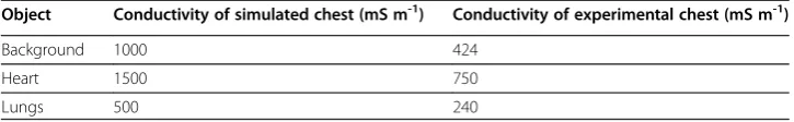
The second column of Table 5 includes the conductivity values of objects inside this numerically simulated chest phantom, as depicted in Figure 2.
As shown in Figure 2, data collection was simulated by 32 finite-sized boundary electro-des for current injection and voltage measurement like ACT3 system [42]. That is, 32 electrodes were arranged counter clockwise, with equally spaces on the boundary of a disk and the first electrode in the position of 3O’clock. The system could inject trigonometric current patterns [38,43] and measure voltages on all 32 electrodes simultaneously. The magnitudes of the injected current patterns were chosen to 1 mA. The simulated boundary values, along with the conductivities of the second column of Table 5, were used to solve the forward problem represented by equations (1) and (2) via FEM and as a result extract the boundary voltages.
Rotating circular target A numerical model including a circular target with a diameter equal to 0.05 of the diameter of its container tank was used to evaluate the accuracy of sinc-convolution reconstructions via calculating some approved parameters. This model is introduced in [2] to evaluate the performance of EIT algorithms. In this model, the conductivity of the target is twice of the homogenous background conductivity.
Simulation data was generated from nine displacements of the target, starting from the medium center and progressing radially outward. The circular medium was surrounded by 16 electrodes. The amplitude of the injected current patterns was 1 mA. Simulated boundary values, were used to solve the forward problem represented by equation (1) and as a result extract the boundary voltages. In this study, to show the effect of measurement noise on the accuracy of under-test algorithms, a uniform noise with amplitude of 0.1 mA was added to resulted boundary data.
Experimental and clinical data
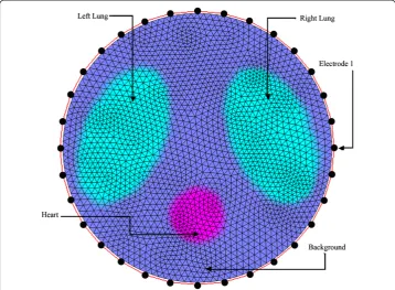
Chest phantom A boundary dataset extracted from real measurements was acquired from the EIDORS [41] website (http://eidors3d.sourceforge.net/data_contrib/jn_chest_phantom/ jn_chest_phantom.shtml). The dataset is gathered by J. Newell, and D. Isaacson [21] in an experiment on a phantom chest consisting of agar heart and lungs in saline tank of radius 15 cm with 32 equally-spaced boundary electrodes of size 1.6 cm height and 2.5 cm width. Table 4 Mesh/grid statistics used in inverse solutions
MODEL Mesh/Grid Number of nodes Number of elements
Thoracic region/Phantom tank/Rotating circular target
Uniform grid 4096 3969
Neonate chest Delaunay Mesh 8257 16256
Table 5 Conductivity values of organs inside chest phantoms
Object Conductivity of simulated chest (mS m-1) Conductivity of experimental chest (mS m-1)
Background 1000 424
Heart 1500 750
Figure 3 shows the configuration of this experimental phantom. The conductivity values of the objects and the saline are included in the third column of Table 5.
Neonate chest data A clinical EIT dataset collected by Heinrich et.al using Gottingen Goe-MF II device on a spontaneously breathing neonate [3] was found in EIDORS[44] website (http://eidors3d.sourceforge.net/data_contrib/if-neonate-spontaneous/index.shtml). This data set includes 220 frames of measured voltages on 16 electrodes using adjacent protocol. As shown in Figure 4, in this measurement the neonate had been lying in prone position with the head turn to the left.
Methods: Performance measures
Convergence rate versus grid size in k-plane
Convergence rate (CR) versus grid size in k-plane, is an important parameter showing the computational efficiency of EIT algorithms in D-bar framework. This calculation is motivated by [22] and calculated using reconstructions of synthetic thoracic region.
Let us denote the true conductivity asγtrueand denote the approximate solution with
a grid of size Ni,i= 1,. . ., 5 in k-plane asγi. The supremum norm of the solution error
may be defined as [22]:
Ei¼ supγtrueγi: ð24Þ
Then, the convergence rate (CR) is defined as [22]:
CRi¼
Ei
Eiþ1: ð25Þ
Note that, to compare sinc-convolution with other non D-bar algorithms such as NOSER, following performance measures are considered.
Accuracy measures versus target positions
Based on the approved test methodology introduced in [2], a scenario is arranged to parametrically evaluate sinc-convolution algorithm. As described below, in this scenario the reconstructions of the rotating circular target are used to calculate a set of accuracy measures that describe the quality of reconstruction algorithms.
Preliminarily, a one-fourth amplitude set γq is computed preliminarily based on reconstructions of circular target. This set contains all image pixels [γ]i, greater than
one-fourth of the maximum amplitude:
γq
h i
i¼
1; if½ γi≥ 1
4maxð Þγ 0; otherwise:
(
ð26Þ
A one-fourth threshold could guarantee to detect most of the visually significant effects in reconstructed conductivity images. The center of gravity ofγandγqare computed and the distances from the medium center to them are calculated as rt and rq respectively.
Then the following performance measuring parameters are calculated.
Amplitude response (AR) measures the ratio of image pixel amplitude in the target to that in the reconstructed image. For a circular target of areaAtwith conductivity
σtin a medium with conductivityσr[2]
AR¼
P
k½ γk At σtσrσr
ð27Þ
In this study, this parameter is normalized so that it AR = 1 for a circular target with σt
σr ¼2in the center of medium.
Position error (PE) represents the extent to which reconstructed image truly represents the position of the circular target in the medium. This parameter is computed as [2]:
PE¼rtrq: ð28Þ
Ringing (RNG) measures the degree of opposite sign area surrounding the main reconstructed target area. For a circleCcentered at center of gravity ofγq, the ringing
could be obtained by [2]:
RNG¼Aout
Ain : ð
29Þ
Resolution (RES) is a measure of the smallest visible object within the reconstructed image. This parameter is be defined as [2]:
RES¼
ffiffiffiffiffiffi
Aq A0
s
; ð30Þ
whereAqandA0denote the number of pixels inγqand entire reconstructed image
respectively.
Shape deformation (SD) measure quantifies the fraction ofγqwhich did not fit
SD¼
X
k2=C
γq
h i
k
P
k γq
h i
k;
ð31Þ
whereCdenotes a circle centered at COG ofγqwith an area equivalent toAq.
Results and discussion
All three methods were implemented within MATLAB and computations were per-formed in a Laptop with 2.4 GHZ CPU and 2 GB RAM. The methods were separately applied to the datasets extracted from aforementioned simulated and real models. To fairly compare the quality of reconstructed conductivity images, iteration parameters were set in a common range for all methods. In addition, same-size grids in k-plane were used in implementation of sinc-convolution and MG.
The following two steps were used to evaluate the quality of sinc-convolution images. First, the synthetic reconstructions were evaluated via efficiency parameters of the preceding section. Next, reconstructions of physical and clinical models were used to validate the parametric assessments.
Results of simulations
Convergence rate
The supremum of reconstruction errors and the required computation times for recon-structions of the synthetic chest phantom using MG and sinc-convolution with differ-ent levels of discretization in k-plane were measured according to equation (24) and then enlisted in third and fourth columns of Tables 6 and 7.
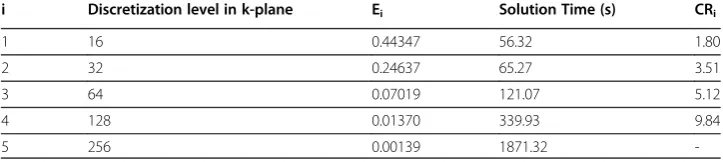
Comparing corresponding accuracies of the reconstruction methods, one can notice that in each case the accuracy of the sinc-convolution method is much better than that of the MG, especially in reconstructions with large grids in k-plane.
Next, for each discretization level in Tables 6 and 7, the corresponding CR values were computed using the corresponding accuracies according to equation (25), and then enlisted in the fifth column of Tables 6 and 7. Comparing the corresponding con-vergence rates of the reconstruction algorithms shows that while the sinc-convolution method has a near-exponential convergence rate in reconstructing the conductivity distribution of the synthetic chest phantom, the MG method only converges with a linear rate, which is considered very slow. This result confirms the stated exponential convergence rate of sinc-convolution [45] as well as the linear convergence rate of MG [22].
performance. Now, it is predictable that to reconstruct higher resolution conductivity images in k-plane, the performance of the sinc-convolution would be finer than that of the MG.
Accuracy
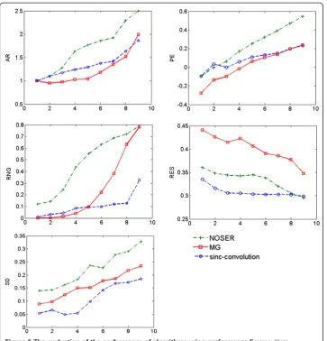
The plots in Figures 5 illustrate different performance figures of each algorithm as functions of radial distance of the moving circular target from the medium center.
The amplitude response of all three methods increase from the center of medium toward the boundary. Remarkable oscillations appear in the amplitude response of MG and NOSER respectively when the target is in the midway point and closest point to the boundary. Despite these two methods, the amplitude response of sinc-convolution is approximately uniform. This consistency guarantees that the same value of
conductivities in different parts of the body contribute equally to the conductivity images produced by sinc-convolution.
For position error, the plots show that when the target moves from the center to the boundary, the PE in MG, NOSER and sinc-convolution increases from−0.3, -0.1 and−0.1 to 0.2, 0.2, and 0.5 respectively. It is clear that the variance of PE in sinc-convolution curve is the closest one to zero. Therefore, the positions of objects are expected to be well recovered in the images reconstructed by sinc-convolution algorithm.
The ringing plots indicate that for all three reconstruction algorithms, this artifact is increased as the target moves from the center of medium toward the boundary. The curves show that, for each position of the target, the maximum RNG is found in the image reconstructed by NOSER.
Resolution plots show that the resolution of the NOSER and sinc-convolution are more uniform and considerably less than that of MG. It is clear that the RES of
sinc-Table 6 Convergence rates and computation times of MG
i Discretization level in k-plane Ei Solution Time (s) CRi
1 16 0.51309 61.12 1.82
2 32 0.28191 81.21 1.70
3 64 0.16582 152.33 2.03
4 128 0.08164 577.29 1.92
5 256 0.04252 3290.01
-Table 7 Convergence rates and computation times of sinc-convolution
i Discretization level in k-plane Ei Solution Time (s) CRi
1 16 0.44347 56.32 1.80
2 32 0.24637 65.27 3.51
3 64 0.07019 121.07 5.12
4 128 0.01370 339.93 9.84
-convolution is fractionally lower than NOSER. Therefore, one may expect to observe most of the conductivity details in sinc-convolution reconstructions.
Shape deformation plots show that the SD of the target in sinc-convolution reconstructions is considerably less than that in images produced by each of other two algorithms. The optimum points for shape deformation in all three methods are near the boundary electrodes.
Aforementioned results evince the suitability of the sinc-convolution algorithm for experimental impedance imaging. In the following, reconstruction of experimental phantom tank via sinc-convolution is presented and compared with that of MG and NOSER.
Results of experiments
Chest phantom
Figure 6 illustrates reconstructions of the phantom tank using all three methods, derived on 64 × 64 grids in z-plane. Note that, this experimental model is reconstructed by product integrals (PI) method in [21] and MG method in [37].
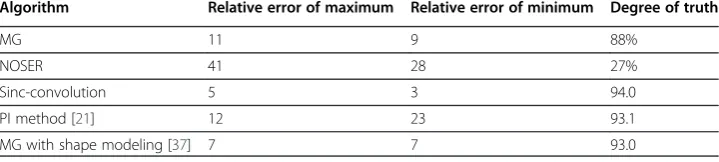
The relative errors in reconstructing heart and lung, using under-test methods are enlisted in the second and third columns of Table 8, respectively. For the purpose of comparison, same parameters for the reconstruction results in [21,37] were computed and then enlisted in fourth and fifth rows of Table 8. It is clear that the relative errors in sinc-convolution reconstructions are the least.
Let define degree of truth (DT) of reconstructions as:
DT ¼Max γrec
Minγrec
Maxð Þ γ Minð Þγ ; ð32Þ
where γrecand γrespectively denote the reconstructed and true conductivity. For each
reconstruction experiment in the first column of Table 8, the corresponding DT is computed using equation (32) and then enlisted in the fourth column of Table 8. Com-paring DT values show that the range of the conductivity distribution of the chest phantom is well recovered in sinc-convolution reconstruction.
It is clear that the representative results of this experiment in Figure 6, confirm the parametric results of Figure 5. The sinc-convolution reconstruction contains a number of sensible features, as described below.
The overall size, position, and the orientation of the organs in the image produced by sinc-convolution are more accurate than that in Figures6(c) and6(d) produced by MG and NOSER.
The sinc-convolution image recovers the separation between the two lungs well while MG and NOSER images do not; MG algorithm overestimates that distance and NOSER underestimates it.
The distortion and blurring of the heart and lungs which are respectively evident in the MG and NOSER images are not appeared respectively in the sinc-convolution image.
Figure 6The experimental reconstructions of chest phantom.The resolutions of the images are 64 × 64. (a) The absolute reconstructed conductivity images using sinc-convolution.(b) The absolute reconstructed conductivity image using MG algorithm. (c) The absolute reconstructed conductivity image using NOSER algorithm.
Table 8 Maximum and minimum values of the chest phantom reconstructions
Algorithm Relative error of maximum Relative error of minimum Degree of truth
MG 11 9 88%
NOSER 41 28 27%
Sinc-convolution 5 3 94.0
PI method [21] 12 23 93.1
The degree of ringing artifact in sinc-convolution image of Figure6(b) is less than that in MG image of Figure6(c) and NOSER image of Figure6(d).
As can be seen, the representative results of this experiment agree very well with accuracy assessment plots in Figure 5. Therefore, the suitability of sinc-convolution for accurate phantom reconstructions is acknowledged.
Neonate chest
Two-dimensional conductivity images of the spontaneously breathing neonate chest are reconstructed using all three methods. The results are depicted in Figure 7. Note that, in these images anterior is at the top and right side of the neonate chest is recon-structed on the left side of the images. Images in the left, middle and right columns of Figure 7 correspond to 45th, 70th and 173th frames of data. These images illustrate the conductivity distribution of the neonate’s thoracic region in three end-inspirations.
It is worth noting that tidal volumes in the neonate’s left lung were reported less than those in his right lung [3]. That is, the conductivity of right lung is expected to be less than that of left one in reconstructed images. Comparing reconstructed images depicted in Figure 7, it is clear that this fact is well recovered in sinc-convolution results. In addition, the sinc-convolution reconstructions seem physiologically most accurate, demonstrating conductivity contrast of heart and lungs and recovering the approximate position of organs with least degree of ringing and deformation. It is evident that the reconstructions of other two methods are relatively distorted. One can easily notice an excellent agree-ment between numerical results obtained via parametric assessagree-ments and the quality of reconstructed images in Figure 7. As a result, the high degree of blurring in MG images may be caused by its low resolution and amplitude response. Similarly, the
Figure 7The two–dimensional reconstructions of neonate chest.First, second and third columns contain reconstructions of 45th, 70thand 173thframes of measured data. Top row: The reconstructed
high degree of deformation of lungs and considerable ringing around them in NOSER images are previously predicted by SD and RNG curves of this method in Figure 5.
Note that, since exact information about the conductivity distribution inside the neonate’s chest is not available, no parametric evaluation and comparison could be planned. However, the representative results of this experiment and their correspondence to parametric evaluations confirm the feasibility of precise clinical EIT reconstruction using sinc-convolution.
Conclusions
The feasibility of accurate practical conductivity image reconstruction via use of sinc-convolution algorithm in D-bar framework was investigated in this study. In the mean-time, the performance of this algorithm was compared with two practical methods including, multigrid and NOSER. In this regard, a two-fold scenario was employed. In the first step, the quality of sinc-convolution reconstructions from noisy boundary data collected on specific synthetic models were evaluated against GREIT agreed accuracy parameters. Results show that the amplitude response and resolution of images are relatively better in sinc-convolution reconstructions. In addition, the effect of the distortions like position error, ringing and shape deformation is considerably reduced in the images produced by sinc-convolution method. Moreover, comparing the conver-gence rate of the convolution with that of MG shows that the new sinc-convolution method is computationally more efficient than its D-bar based competitor.
In the second step, conductivity images of an experimental phantom chest were reconstructed using all three methods. Excellent agreement between their qualities and parametric assessment results support the sinc-convolution suitability for experimental EIT. As a complementary experiment, two-dimensional conductivity images of the chest cross-section of a spontaneously breathing neonate were reconstructed using all three methods. A watchful comparison shows that the related physiological problem is best revealed in sinc-convolution images. In addition, position, size and orientation of organs are well recovered in sinc-convolution images.
These reasons, suggest the sinc-convolution as an efficient algorithm for precise clinical EIT applications.
Appendix A: Computingγbest
The best constant conductivity approximation to the measured boundary data can be computed according to the following formula, which is found in [9,21].
Letρdenote the resistivity (the reciprocal of the conductivity), then for a medium of homogenous resistivity, the voltage on thelth electrode from thekth current pattern is proportional to the voltage arising from a constant distribution of one. That is
Vlkð Þ ¼ρ ρVlkð Þ1 : ðA:1Þ
Let {Ulk} denote the set of measured voltage data andVlk(ρ) the calculated voltage on
min ρ
XL1
k¼1
XL
l¼1
ρVlkð Þ 1 Ulk
2
: ðA:2Þ
The solutionρbestto this minimization problem is given by
ρbest ¼ P L1
k¼1
PL l¼1
Vk lð Þ1 Ulk
P L1
k¼1
PL l¼1
Vlkð Þ1
2 : ð
A:3Þ
The best constant conductivity is thenγbest ¼ 1 ρbest.
Abbreviations
EIT: Electrical impedance tomography; PI: Product integral; MG: Multi-grid; CR: Convergence rate; DT: Degree of truth; AR: Amplitude response; PE: Position error; RES: Resolution; RNG: Ringing; SD: Shape deformation.
Competing interests
The authors declare that they have no competing interests.
Authors’contributions
MA designed and performed the experiments and numerical modeling; ARNN analyzed the experiments and numerical modeling. Both of authors read and approved the final manuscript.
Acknowledgements
Authors appreciate professor Jin Keun Seo for helpful discussions. Also, the authors thank the anonymous referees for their in-depth reviews and constructive comments.
Received: 6 January 2012 Accepted: 7 May 2012 Published: 20 June 2012
References
1. Webster JG:Electrical impedance tomography. 1st edition. New York: Adam Hilger; 1990.
2. Adler A, Arnold JH, Bayford R, Borsic A, Brown B, Dixon P, Faes TJC, Frerichs I, Gagnon H, Gärber Y,et al:GREIT: a unified approach to 2D linear EIT reconstruction of lung images.Physiol Meas2009,30(6):S35.
3. Heinrich S, Schiffmann H, Frerichs A, Klockgether-Radke A, Frerichs I:Body and head position effects on regional lung ventilation in infants: an electrical impedance tomography study.Intensive Care Med2006,
32(9):1392–1398.
4. Flores-Tapia D, O'Halloran M, Pistorius S:A bimodal reconstruction method for breast cancer imaging.
Prog Electromagn Res2011,118:461–486.
5. Elke G, Pulletz S, Schädler D, Zick G, Gawelczyk B, Frerichs I, Weiler N:Measurement of regional pulmonary oxygen uptake—a novel approach using electrical impedance tomography.Physiol Meas2011,32(7):877. 6. Calderon AP:On inverse boundary value problem.Math App Comput2006,25(2):133–138.
7. Kotre CJ:EIT image reconstruction using sensitivity weighted filtered backprojection.Physiol Meas1994, 15(2A):A125.
8. Wang H, Xu G, Zhang S, Yin N, Yan W:Implementation of generalized back projection algorithm in 3-D EIT.
IEEE Trans Magn2011,47(5):1466–1469.
9. Cheney M, Isaacson D, Newell JC, Goble J, Simske S:Noser: an algorithm for solving the inverse conductivity problem.Int J Imaging Syst Technol1990,2:66–75.
10. Lionheart WRB:EIT reconstruction algorithms: Pitfalls, challenges and recent developments.Physiol Meas2004, 25(1):125–142.
11. Hua P, Woo EJ, Webster JG, Tompkins WJ:Iterative reconstruction methods using regularization and optimal current patterns in electrical impedance tomography.IEEE Trans Med Imaging1991,10(4):621–628.
12. Kallman JS, Berryman JG:Weighted least-squares criteria for electrical impedance tomography.IEEE Trans Med Imaging1992,11(2):284–292.
13. Kaipio JP, Kolehmainen V, Somersalo E, Vauhkonen M:Statistical inversion and Monte Carlo sampling methods in electrical impedance tomography.Inverse Problems2000,16(5):1487–1522.
14. Rao L, He R, Wang Y, Yan W, Bai J, Ye D:An efficient improvement of modified Newton–Raphson algorithm for electrical impedance tomography.IEEE Trans Magn1999,35(3 PART 1):1562–1565.
15. Somersalo E, Cheney M, Isaacson D, Isaacson E:Layer stripping: A direct numerical method for impedance imaging.Inverse Problems1991,7(6):899–926.
16. Nachman AI:Global uniqueness for a two-dimensional inverse boundary value problem.Ann Math1996,143 (1):71–96.
18. Abbasi A, Vosoghi Vahdat B:Improving forward solution for 2D block electrical impedance tomography using modified equations.Sci Res Essays2010,5(11):1260–1263.
19. Abbasi A, Vosoghi Vahdat B:A non-itertive linear inverse solution for block approach in EIT.
Comput Sci2010,1:190–196.
20. Nachman AI, Ablowitz MJ:Multidimensional inverse-scattering method.Stud Appl Math1984, 71(3):243–250.
21. Isaacson D, Mueller JL, Newell JC, Siltanen S:Reconstructions of chest phantoms by the D-bar method for electrical impedance tomography.IEEE Trans Med Imaging2004,23(7):821–828.
22. Knudsen K, Mueller J, Siltanen S:Numerical solution method for the dbar-equation in the plane.J Comput Phys
2004,198(2):500–517.
23. Siltanen S, Mueller J, Isaacson D:An implementation of the reconstruction algorithm of A Nachman for the 2D inverse conductivity problem.Inverse Problems2000,16(3):681–699.
24. Mueller JL, Siltanen S, Isaacson D:A direct reconstruction algorithm for electrical impedance tomography.
IEEE Trans Med Imaging2002,21(6):555–559.
25. Vainikko G:Fast solvers of the Lippmann-Schwinger equation.Direct and Inverse problems of Mathical Physics
2000,5:423–440.
26. DeAngelo M, Mueller JL:2D D-bar reconstruction of the human chest and tank data using an improved approximation to the scattering transform.Physiol Meas2010,31:221–232.
27. Abbasi M, Naghsh-Nilchi AR:Iterative sinc-convolution method for solving planar D-bar equation with application to EIT.Biomed Eng: Int J Numer Meth,2012,28(8):838–860.
28. Brown RM, Uhlman G:Uniqueness in the inverse conductivity problem for non-smooth conductivities in two dimensions.Commun Partial Differ Eq1997,22(5):1009–1027.
29. Astala K, Mueller JL, Päivärinta L, Siltanen S:Numerical computation of complex geometrical optics solutions to the conductivity equation.Appl Comput Harmon Anal2010,29(1):2–17.
30. Beals R, Coifman RR:The D-bar approach to inverse scattering and nonlinear evolutions.Physica D: Nonlinear Phenomena1986,18(1–3):242–249.
31. Faddeev LD:Increasing solutions of the schrodinger equation.Sov Phys Dokl1965,10:1033–1035. 32. Knudsen K, Lassas M, Mueller JL, Siltanen S:Regularized d-bar method for the inverse conductivity problem.
Inverse Problems and Imaging2009,3(4):599–624.
33. Mueller JL, Siltanen S:Direct reconstructions of conductivities from boundary measurements.SIAM J Sci Comput2003,24(4):1232–1263.
34. Isaacson D, Mueller JL, Newell JC, Siltanen S:Imaging cardiac activity by the D-bar methd for electrical impedance tomography.Physiol Meas2006,27:S43–S50.
35. Du K, Nevanlinna O:A note onℝ-linear GMRES for solving a class ofℝ-linear systems.Numer Linear Algebra Appl2011. doi:10.1002/nla.769.
36. Murphy EK, Mueller JL, Newell JC:Reconstructions of conductive and insulating targets using the D-bar method on an elliptical domain.Physiol Meas2007,28(7):S101–S114.
37. Murphy EK, Mueller JL:Effect of domain shape modeling and measurement errors on the 2-D D-bar method for EIT.IEEE Trans Med Imaging2009,28(10):1576–1584.
38. Cheng KS, Isaacson D, Newell JC, Gisser DG:Electrode models for electric current computed tomography.
IEEE Trans Biomed Eng1989,36(9):918–924.
39. Paulson K, Breckon W, Pidcock M:Electrode modelling in electrical impedance tomography.SIAM J Appl Math
1992,52(4):1012–1022.
40. Schroberl J:NETGEN: an advancing front 2D/3D-mesh generator based on abstract rules.Comput Vis Sci1997, 1:41–52.
41. EIDORS:Calibrated chest shaped targets in 2D circular tank with ACT 3 EIT system.[http://eidors3d. sourceforge.net/data_contrib/ds_tank_phantom/ds_tank_phantom.shtml]
42. Edic PM, Saulnier GJ, Newell JC, Isaacson D:A real-time electrical impedance tomograph.IEEE Trans Biomed Eng
1995,42(9):849–859.
43. Isaacson D:Distinguishability of conductivities by electric current computed tomography.IEEE Trans Med Imaging1986,MI-5(2):91–95.
44. EIDORS:EIT images of spontaneously breathing neonate. [http://eidors3d.sourceforge.net/data_contrib/if-neonate-spontaneous/index.shtml]
45. Stenger F:Numerical methods based on sinc and analytic functions. 1st edition. New York: Springer; 1993.
doi:10.1186/1475-925X-11-34
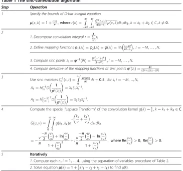
![Figure 3 The experimental chest phantom including agar heart and lungs in a saline tank [41].heart and lungs are suspended in a saline bath](https://thumb-us.123doks.com/thumbv2/123dok_us/9140721.1907846/14.595.118.478.463.697/figure-experimental-chest-phantom-including-saline-suspended-saline.webp)